Chemical Pesticides: Mode of Action and Toxicology - Chapter 2 pptx
Bạn đang xem bản rút gọn của tài liệu. Xem và tải ngay bản đầy đủ của tài liệu tại đây (131.95 KB, 19 trang )
chapter two
Why is a toxicant poisonous?
Theophrastus Bombastus von Hohenheim, better known in history as
Paracelsus, who was born in the Swiss village of Einsiedeln in 1493 and died
in 1541, taught us that the severity of a poison was related to the dose (see
Strathern, 2000). His citation “All substances are poisons; there is none which
is not a poison. The right dose differentiates a poison from a remedy” is
found in the first chapter of almost all textbooks of toxicology or pharma-
cology. However, the molecular theory was formulated more than 300 years
later, and the law of mass action not until after the middle of the 19th century.
Real rational toxicology and pharmacology are dependent on these laws,
and hence could not develop properly before they were known.
Paracelsus’ idea that all substances are poisons is, of course, correct; even
water, air, and sugar are poisons in sufficient amounts, but by looking at the
chemical structures of typical poisons, and trying to sort out the reactions
they tend to be involved in, we can roughly put them into seven categories.
By using the molecular theory, the law of mass action, and our knowledge of
the nature of the chemical processes in organisms, we can condense biochemical
toxicology to three sentences, and about seven types of reactions:
1. Toxic molecules react with biomolecules according to the common laws
of chemistry and physics, so that normal processes are disturbed.
2. The symptoms increase in severity with increasing concentration of
the toxicant at the site of reaction.
3. This concentration increases with increasing dose.
2.1 Seven routes to death
The chemist may prefer to classify toxicants according to their chemical
structure, the doctor according to the organ they harm, the environmentalist
according to their stability in the environment, and so forth. The biochemist
may use a different classification, and we will approach the toxicology of
pesticides from the biochemist’s perspective. Because of point 1 above, and
because the cells in all organisms are very similar, it is possible to classify
©2004 by Jørgen Stenersen
toxicants into roughly seven categories according to the type of biomolecule
they react with. Toxicants in the same category do not need to be chemically
related, and one substance may act through several mechanisms. The fol-
lowing simple classification is based on the more comprehensive texts of
Ecobichon (2001) and Gregus and Klaassen (2001).
2.1.1 Enzyme inhibitors
The toxicant may react with an enzyme or a transport protein and inhibit
its normal function. Enzymes may be inhibited by a compound that has a
similar, but not identical structure as the true substrate; instead of being
processed, it blocks the enzyme. Typical toxicants of this kind are the car-
bamates and the organophosphorus insecticides that inhibit the enzyme
acetyl cholinesterase. Some extremely efficient herbicides that inhibit
enzymes important for amino acid synthesis in plants, e.g., glyphosate and
glufosinate, are other good examples in this category.
Enzyme inhibitors may or may not be very selective, and their effects
depend on the importance of the enzyme in different organisms. Plants lack
a nervous system and acetylcholinesterase does not play an important role
in other processes, whereas essential amino acids are not produced in ani-
mals. Glyphosate and other inhibitors of amino acid synthesis are therefore
much less toxic in animals than in plants, and the opposite is true for the
organophosphorus and carbamate insecticides.
Sulfhydryl groups are often found in the active site of enzymes. Sub-
stances such as the Hg
++
ion have a very strong affinity to sulfur and will
therefore inhibit most enzymes with such groups, although the mercury ion
does not resemble the substrate. In this case, the selectivity is low.
2.1.2 Disturbance of the chemical signal systems
Organisms use chemicals to transmit messages at all levels of organization,
and there are a variety of substances that interfere with the normal function-
ing of these systems. Toxicants, which disturb signal systems, are very often
extremely potent, and often more selective than the other categories of poi-
sons. These toxicants may act by imitating the true signal substances, and
thus transmit a signal too strongly, too long lasting, or at a wrong time. Such
poisons are called agonists. A typical agonist is nicotine, which gives signals
similar to acetylcholine in the nervous system, but is not eliminated by
acetylcholinesterase after having given the signal. Other quite different ago-
nists are the herbicide 2,4-D and other aryloxyalkanoic acids that mimic the
plant hormone auxin. They are used as herbicides. An antagonist blocks the
receptor site for the true signal substance. A typical antagonist is succinylcholin,
which blocks the contact between the nerve and the muscle fibers by reacting
with the acetylcholine receptor, preventing acetylcholine from transmitting the
signal. Some agonists act at intracellular signal systems. One of the strongest
man-made toxicants, 2,3,7,8-tetrachlorodibenzodioxin, or dioxin, is a good
©2004 by Jørgen Stenersen
example. It activates the so-called Ah receptor in vertebrates, inducing several
enzymes such as CYP1A1 (see p. 181). Organisms use a complicated chemical
system for communication between individuals of the same species. These
substances are called pheromones. Good examples are the complicated system
of chemicals produced by bark beetles in order to attract other individuals
to the same tree so that they can kill them and make them suitable as
substrates. Man-made analogues of these pheromones placed in traps are
examples of poisons of this category. The kairomons are chemical signals
released by individuals of one species in order to attract or deter individ-
uals of another. The plants’ scents released to attract pollinators are good
examples.
Signals given unintentionally by prey or a parasite host, which attract
the praying or parasitizing animal, are important. A good example is CO
2
released by humans, which attracts mosquitoes. The mosquito repellent
blocks the receptors in the scent organ of mosquitoes.
2.1.3 Toxicants that generate very reactive molecules that destroy
cellular components
Most redox reactions involve exchange of two electrons. However, quite a
few substances can be oxidized or reduced by one-electron transfer, and
reactive intermediates can be formed. Oxygen is very often involved in such
reactions. The classical example of a free radical-producing poison is the
herbicide paraquat, which steals an electron from the electron transport chain
in mitochondria or chloroplasts and delivers it to molecular oxygen. The
superoxide anion produced may react with hydrogen superoxide in a reac-
tion called the Fenton reaction, producing hydroxyl radicals. This radical is
extremely aggressive, attacking the first molecule it meets, no matter what
it is. A chain reaction is started and many biomolecules can be destroyed by
just one hydroxyl radical. Because one paraquat molecule can produce many
superoxide anions, it is not difficult to understand that this substance is toxic.
Copper acts in a similar way because the cupric ion (Cu
++
) can take up one
electron to make the cuprous cation (Cu
+
) and give this electron to oxygen,
producing the superoxide anion (O
2
·
–
).
Free radical producers are seldom selective poisons. They work as an
avalanche that destroys membranes, nucleic acids, and other cell structures.
Fortunately, the organisms have a strong defense system developed during
some billion years of aerobic life.
2.1.4 Weak organic bases or acids that degrade the pH gradients
across membranes
Substances may be toxic because they dissolve in the mitochondrial mem-
brane of the cell and are able to pick up an H
+
ion at the more acid outside,
before delivering it at the more alkaline inside. The pH difference is very
important for the energy production in mitochondria and chloroplasts, and
©2004 by Jørgen Stenersen
this can be seriously disturbed. Substances like ammonia, phenols, and acetic
acid owe their toxicity to this mechanism. Selectivity is obtained through
different protective mechanisms. In plants, ammonia is detoxified by
glutamine formation, whereas mammals make urea in the ornithine cycle.
Acetic acid is metabolized through the citric acid cycle, whereas phenols can
be conjugated to sulfate or glucuronic acid. Phenols are usually very toxic
to invertebrates, and many plants use phenols as defense substances.
2.1.5 Toxicants that dissolve in lipophilic membranes and
disturb their physical structure
Lipophilic substances with low reactivity may dissolve in the cell membranes
and change their physical characteristics. Alcohols, petrol, aromatics, chlorinated
hydrocarbons, and many other substances show this kind of toxicity. Other,
quite unrelated organic solvents like toluene give very similar toxic effects.
Lipophilic substances may have additional mechanisms for their toxicity.
Examples are hexane, which is metabolized to 2,5-hexandion, a nerve poison,
and methanol, which is very toxic to primates.
2.1.6 Toxicants that disturb the electrolytic or osmotic balance
or the pH
Sodium chloride and other salts are essential but may upset the ionic balance
and osmotic pressure if consumed in too high doses. Babies, small birds, and
small mammals are very sensitive. Too much or too little in the water will
kill aquatic organisms.
2.1.7 Strong electrophiles, alkalis, acids, oxidants, or reductants that
destroy tissue, DNA, or proteins
Caustic substances like strong acids, strong alkalis, bromine, chlorine gas,
etc., are toxic because they dissolve and destroy tissue. Many accidents
happen because of carelessness with such substances, but in ecotoxicology
they are perhaps not so important. More interest is focused on electrophilic
substances that may react with DNA and induce cancer. Such substances are
very often formed by transformation of harmless substances within the body.
Their production, occurrence, and protection mechanisms will be described
in some detail later.
2.2 How to measure toxicity
2.2.1 Endpoints
In order to measure toxicity, it is important to know what to look for. We
must have an endpoint for the test. An endpoint can be very precise and easy
©2004 by Jørgen Stenersen
to monitor, such as death, or more sophisticated, for instance, lower learning
ability or higher risk for contracting a disease. Some endpoints are
all-or-none endpoints. At a particular dose some individuals will then get
the symptoms specified in the definition of the endpoint and others do not.
Tumors or death are such all-or-none endpoints. Such endpoints are often
called stochastic, whereas endpoints that all individuals reach, to varying but
dose-dependent degrees, are called deterministic endpoints. Intoxication by
alcohol is a good example. We use the term response for the stochastic
all-or-none endpoints and the term effect for gradual endpoints.
2.2.1.1 Endpoints in ecotoxicology and pest control
The fundamental endpoints for nonhuman organisms are:
• Death
• Reduced reproduction
• Reduced growth
• Behavioral change
These endpoints are, of course, connected.
Reduced reproduction is probably the most important endpoint in
ecotoxicological risk assessments, whereas in pest control, death or changes
in behavior are the most important. We simply want to kill the pest or make
it run away. Toxicity tests are often based on what we call surrogate end-
points. We measure the level of an enzyme and how its activity is increased
(e.g., CYP1A1) or reduced (acetylcholinesterase), how a toxicant reduces the
light of a phosphorescent bacterium, or how much a bacterium mutates.
Such endpoints are not always intuitively relevant to human health or envi-
ronmental quality, but much research is done in order to find easy and
relevant endpoints other than the fundamental ones.
2.2.1.2 Endpoints in human toxicology
In human toxicology, we have a lot more sophisticated endpoints related to
our well-being and health. At the moment, cancer is the most feared effect
of chemicals, and tests that can reveal a chemical’s carcinogenicity are always
carried out for new pesticides. Other tests that may reveal possible effects
on reproduction and on the fetus are important. Endpoints such as immu-
nodeficiency, reduced intelligence, or other detrimental neurological effects
will play an important role in the future. The problem is that almost all
endpoints in human toxicology are surrogate endpoints, and elaborate and
dubious extrapolations must be done. The new techniques under develop-
ment that make it possible to determine the expression of thousands of genes
by a simple test will very soon be used in toxicological research, but the
interpretation problems will be formidable.
©2004 by Jørgen Stenersen
2.2.2 Dose and effect
The law of mass action tells us that the amount of reaction products and the
velocity of a chemical reaction increase with the concentrations of the reac-
tants. This means that there is always a positive relation between dose and
the degree of poisoning. A greater dose gives a greater concentration of the
toxicant around the biomolecules and therefore more serious symptoms
because more biomolecules react with the toxicant and at a higher speed.
This simple and fundamental law of mass action is one of the reasons why
a chemist does not believe in homeopathy. It is also the reason why Paracel-
sus (1493–1541) was right when saying “All substances are poisons; there is
none which is not a poison. The right dose differentiates a poison from a
remedy” (Strathern, 2000). The connection between dose or concentration of
the toxicant and the severity of the symptoms is fundamental in toxicology.
By using the law of mass action, we get the following equilibrium and
mathematical expression:
B + T
BT
K
or if C = C
B
+ C
BT
The target biomolecule (B) at the concentration C
B
reacts with the toxicant
(T) at the concentration C
T
to give the destroyed biomolecule (BT) at the
concentration C
BT
. The reaction may be reversible, as indicated by the double
arrow. C is the total concentration of the biomolecule and K is the equilibrium
constant. If the onset speed of the symptoms is proportional with the disap-
pearance rate of the biomolecules (–dC
B
/dt), we get this simple mathematical
expression telling us that the higher the concentration of the toxicant is, the
faster C
B
will decrease and the symptoms appear:
k
+1
is the velocity constant for the reaction.
These simple formulae illustrate that higher concentrations of a toxicant
give a lower amount of the biomolecule and thus stronger symptoms. The
onset of symptoms may start when C
B
is under a certain threshold or C
BT
is
above a threshold.
The real situation is more complicated. The toxicant may react with many
different types of biomolecules. It may be detoxified or need to be trans-
formed to other molecules before reacting with the target biomolecule.
K
CC
C
BT
BT
=
⋅
CK
C
CK
B
T
=⋅
+
−=⋅⋅
+
dC
dt
kCC
B
BT1
©2004 by Jørgen Stenersen
2.2.3 Dose and response
The sensitivity of the individuals in a group is different due to genetic
heterogenicity as well as difference in sex, age, earlier exposure, etc. There-
fore, if the effect of a toxicant is plotted against the dose, every individual
will get a curve that is more or less different from those of other individuals.
In Figure 2.1, some effect on eight individuals is shown. The difference is
exaggerated in order to elucidate the points.
Figure 2.1 illustrates a hypothetical example. The effect may be any
measurable symptom that has a graded severity. Three individuals seem to
be very sensitive, whereas one or two are almost resistant. This figure leads
us to a very important concept called response. Response (r) is defined as the
number of individuals getting symptoms higher than a defined threshold.
If we decide that the symptom threshold should be 50, we observe that at
doses 3, 10, 20, and 30 the response will be 2, 4, 6, and 6, respectively. When
determining the response, we just count how many individuals have the
required or higher symptoms.
The relative response (p) is the number of responding individuals
divided by the total number given a certain dose. At the marked dose levels
in Figure 2.1, the relative responses are 0.25, 0.5, 0.75, and 0.75, respectively.
These numbers may be multiplied by 100 to give the percent response.
We very often measure all-or-none symptoms (dead or alive, with tumor
or without tumor, numbers of fetus with injury or normal ones) in toxicology.
Such symptoms are not gradual. We then have to expose groups of individ-
uals with different doses (D) and determine the number of responding indi-
viduals (r) and the relative number (p).
If we have many groups with a high number of individuals and then
plot the relative response against the dose, we very often get an oblique
Figure 2.1 A hypothetical example of the effects on eight individuals of a toxicant at
different doses.
0 10 20 303
0
25
50
75
100
Dose
Effect
©2004 by Jørgen Stenersen
S-shaped graph, with an inflection point at 50% response. The graph may
be made symmetrical by plotting log dose instead of dose. Furthermore, the
S-shaped graphs can be changed into straight lines by transforming the
responses to probit response. We then presuppose that the sensitivity of the
organisms has a normal distribution, which predicts that most individuals
have average sensitivity, a few are very robust, very few are almost resistant,
and some have high sensitivity.
The log transformation of dose or concentration is easily done with a
pocket calculator. Using the formula for the inverse normal distribution in
the data sheet Excel, one can easily do the calculation of the probit values.
The mean or median is set to 5 and the standard deviation to 1, i.e., the
formula will look like this:
=NORMINV (relative response; 5 ;1)
By writing the relative response into the formula, Excel will return the probit
value.
Note that the probit of 0.5 (50% response) is 5, and the probit of 0.9 (90%
response) is 6.282. The reader should try other values if Excel is available.
Note also that the probit of 0 is –∞, whereas the probit of 1 is +∞. Values of
0 or 100% response are therefore useless in this plot. Figure 2.2 and Figure
2.3 show the essence of some dose–response curves.
Figure 2.3a and b shows a case with sensitive and resistant flies mixed
50:50. The same data are used in both plots.
Figure 2.2a to c and Figure 2.3a and b show that the transformation of
the doses to log dose, and the use of probit units for responses, makes it
much easier to interpret the graphs. However, there are several difficulties
with dose–response graphs.
Mathematically, the probit of a value P is Y in the integral
It cannot be expressed as a simple function, and some mathematical skill
is necessary to interpret its meaning. Therefore, the much simpler logit
transformation L = ln{P/(1 – P)} is often used. The logit values (L) can be
calculated from the relative response values (P) with a pocket calculator. The
logit transformation also gives almost straight lines if the sensitivity is nor-
mally distributed. The most serious problem with dose–response graphs,
however, is not this mathematical inconvenience. The low reproducibility is
a more serious problem. As an example, if you know exactly the LD50 (lethal
dose in 50% of the population) and give this to 10 animals, the probability
that 5 die is only 0.246. The confidence intervals of the responses for the
same dose, or for the doses calculated to give a specified response (e.g.,
Pedu
u
Y
=
−
−∞
−
∫
1
2
1
2
5
2
π
©2004 by Jørgen Stenersen
Figure 2.2 Dose–response relationships drawn on three different models for four
populations. (a) Doses and responses in linear scale. (b) Doses in log scale and
responses in linear scale. (c) Doses in log scale and responses in probits. (1) Sensitive
population with normally distributed sensitivity and LD50 = 2.5 units. (2) A mixed
population with 75% of (1) and 25% resistant individuals. (3) Intermediate sensitive
population with normally distributed sensitivity, but more scattered than (1), and
LD50 = 5 units. (4) Less sensitive, but normally distributed population, similar to (1),
but with LD50 = 6.5 units.
0 4 8 12 16
0
20
40
60
80
100
Dose
Response (%)
a
1
2
3
4
-0.35 0.05 0.45 0.85 1.25
0
20
40
60
80
100
Dose (log)
Response (%)
b
1
2
3
4
-0.35 0.05 0.45 0.85 1.25
2.50
3.75
5.00
6.25
c
Dose (log)
Response (probit)
1
2
3
4
©2004 by Jørgen Stenersen
LD50), will be large and are not easily calculated without special data pro-
grams. Another problem is that responses of 0 or 100%, which very often
occur in practical experiments, give probit (or logit) values of –∞ or +∞ that
cannot be plotted into the diagram. The outcome of such an experiment may
be disappointing if nice curves are expected. Let us look at a case study
before describing the scatter problem in more detail. A standard description
of probit analyses can be found in Finney (1971).
2.2.3.1 Dose–response curves for the stable fly
As a real-life example, we can use an experiment done by myself as part of
my master’s thesis in 1962 (Stenersen and Sømme, 1963). The stable fly
(Stomoxys calcitrans) is an important insect pest in husbandry. In the Nordic
countries it is an indoor pest, present as many small, partially isolated
populations. From 1950 to 1965 it was controlled with DDT, but resistance
soon became a problem. A strain (R) of stable fly resistant to the DDT and
related insecticides such as DDD and methoxychlor was compared with a
sensitive (S) strain. Males from the R strain were then crossed with females
from the S strain and the offspring (F1 of S × R) were tested. They were as
sensitive as the S strain. The F1 flies were allowed to interbreed and the
Figure 2.3 Dose–response curves for susceptible and resistant flies and a mixture
(50:50) of susceptible and resistant flies. (a) Doses and responses on linear scales. (b)
Doses on log scale and responses on probit scale.
0 20 40 60 80 100
0
25
50
75
100
Sensitive
Mixture
Resistant
Dose
Response (%)
a
-0.5 0.0 0.5 1.0 1.5 2.0
3
5
7
Resistant
Sensitive
Mixture
Dose (log)
Response (probit)
b
©2004 by Jørgen Stenersen
resulting F2 generation was tested. As seen from Figure 2.4, these flies had
a very heterogeneous sensitivity against DDD. About 75% (probit value of
5.674490) were quite sensitive, whereas 25% were almost impossible to kill with
DDD. This result is expected if just one (recessive) gene is involved in the
resistance mechanism. The other DDT group insecticides gave similar results.
2.2.3.2 Scatter in dose–response data
The figure of the Stomoxys strains also illustrates the wide scatter expected
for the response data. Each point is based on 20 individuals, i.e., more than
400 flies plus controls (60) were used in this small experiment. The scatter
is formidable in spite of the great number of flies used. The reason is the
stochastic nature of the outcome. For instance, the probability (P) of getting
exactly 15 dead flies by using a dose that should kill 75% is only P = 0.203.
It is much more probable that we get another “wrong” value. These results
may be calculated from the binomial formula
where n = 20, number of insects tested in a group; r = 15, number of insects
dying; p = 75/100, the expected value of relative response when a huge
number of insects was used; and ! is the faculty sign (e.g., n! = n × (n – 1) ×
(n – 2) … 3 × 2 × 1). It may be calculated that P = 0.203, which is the probability
of obtaining a response of r = 15 in an experiment where p = 0.75 and n =
20. An outlier (see Figure 2.4), as that obtained at 4 µg/fly (log dose = 0.602),
with a response of r = 18 (90% mortality instead of the expected 75%), has
a probability of 0.0669, i.e., is expected in as many as 7 experiments out of
100. Such uncertainties are inherent in dose–response relationships and have
nothing to do with experimental errors, which may also be a source of
scattering.
Figure 2.4 Dose–response relationships of Stomoxys calcitrans treated with the DDT
analogue DDD. S, susceptible strain; R, resistant strain; F
2
, second generation from
crosses of S and R.
-1.75 -1.25 -0.75 -0.25 0.25 0.75 1.25 1.75
2.5
5.0
7.5
5.67
R
S
F
2
75%
Dose (log g/fly)
Response (Probit)
P
n
nr r
pp
rnr
=
−×
××−
−
!
()!!
()
()
1
©2004 by Jørgen Stenersen
2.2.4 LD50 and related parameters
The statistical problems in making good dose–response curves can only be
overcome by using many organisms in the experiment. A better method may
be to determine one dose, for instance, the dose that is expected to kill or
harm 50% of the individuals, and not to construct a graph. This can be done
satisfactorily with much fewer individuals. The latter method is definitely
better when studying vertebrates. Most countries have strict legislation con-
cerning the use of vertebrates in research, and it is difficult to get permission
to do experiments involving hundreds of animals. Furthermore, most ver-
tebrates suitable for research are expensive. Therefore, we seldom find
graphs of dose–response relationships on mammals in the more recent sci-
entific literature. More often, we find a value called LD50 that can be deter-
mined with reasonable accuracy by using few individuals. LD50 is the dose
expected to kill half of the exposed individuals. Sometimes we are interested
in determining the doses that kill 90 or 10%, etc., and these doses are called
LD90 and LD10, respectively. They can easily be determined from a
dose–response curve, but these values are less accurate than LD50. If we
study endpoints other than death, we use the term ED50 (effective dose in
50% of the population), and if we study concentrations and not doses, we use
the terms LC50 (lethal concentration in 50% of the population) and EC50
(effective concentration in 50% of the population). Protocols for determina-
tion of LD50 for rodents are available in order to minimize the number of
animals necessary for a satisfactory determination. According to Commis-
sion of the European Communities’ Council Directive 83/467/EEC, 20 rats
may be sufficient for an appropriate LD50 determination. LD50 values are
often given as milligram of toxicant per kilogram of body weight of the
test animals, assuming that twice as big a dose is necessary to kill an animal
of double weight. It is therefore easier to compare toxicity data from dif-
ferent species, life stage, or sex. The LD50 values or the related values
should not be taken as accurate figures owing to the intrinsic nature of
these parameters, as well as the difficulties of determination. Even if you
know the exact LD50 value, for example, of parathion to mice (LD50 =12
mg/kg according to The Pesticide Manual), and give these doses to a group
of animals, for instance, n = 10, the probability that r = 5 will die is only
P = 0.246. This can easily be calculated from the binomial formula. How-
ever, you can be confident that between 1 and 9 will die (P = 0.998). LD50
values are therefore very useful if you do not need to know the exact
number of fatalities, but merely want to describe the toxicity of a compound
by one figure. Complicated statistical methods are needed to determine
the true confidence limits of LD50. Many statistical methods are described
in the books of Finney (1971) and Hewlett and Plackett (1979). Data pro-
grams may be used, e.g., Sigmaplot
®
or Graphpad Prism
®
. A simple pro-
gram in BASIC is available (Trevors, 1986), whereas Caux and More (1997)
describe the use of Microsoft Excel
®
.
Table 2.1 shows how toxicants are classified according to their LD50.
©2004 by Jørgen Stenersen
2.2.5 Acute and chronic toxicity
An important distinction has to be made between acute and chronic toxicity.
Substances that are eliminated very slowly and therefore accumulate if
administered in several small doses over a long time may, when the total
dose is large enough, cause symptoms. A good example is cadmium that
accumulates in the kidneys. Another example is organophosphates that in
repeated small doses eventually inhibit acetylcholinesterase more than 80%,
which will produce neurotoxic symptoms. Because the inhibition is partly
irreversible, many small doses may cause poisoning even though the poison
itself does not accumulate. Other poisons (e.g., ethanol) may be given in
large, but sublethal doses for years before any sign of chronic toxicity is
observed (liver cirrhosis), whereas the acute toxicity results in well-known
mental disturbances. In many cases, acute or subacute doses may give
chronic symptoms or effects many years after poisoning (cigarette smoking
and cancer) or effects in the following generation (stilbestrol may give vag-
inal cancer in female offspring at puberty).
We use the following terms:
Acute dose — The dose is given during a period shorter than 24 h.
Subacute dose — The doses are given between 24 h and 1 month.
Subchronical dose — The doses are given between 1 and 3 months.
Chronical dose — The doses are given for more than 3 months.
These terms apply to mammals, whereas the times are shorter for
short-lived animals or plants used in tests. The dose of a pesticide toward a
pest will usually be acute, whereas the dose that consumers of sprayed food
will be exposed to is chronic.
2.3 Interactions
One toxicant may be less harmful when taken together with another chem-
ical. If we use blindness as an endpoint for methanol poisoning, then whisky
Table 2.1 Common Classification of Substances
Toxicity Class LD50 (mg/kg) Examples, LD50 (mg/kg)
Extremely toxic Less than 1.0 Botulinum toxin: 0.00001
Aldicarb: 1.0
Very toxic 1–50 Parathion: 10
Moderately toxic 50–500 DDT: 113–118
Weakly toxic 500–5000 NaCl: 4000
Practically nontoxic 5000–15,000 Glyphosate: 5600
Ethanol: 10,000
Nontoxic More than 15,000 Water
©2004 by Jørgen Stenersen
or other drinks that contain ethanol would reduce the toxicity of methanol
considerably. When ethanol is present, methanol is metabolized more slowly
to formaldehyde and formic acid, which are the real harmful substances.
Ethanol is therefore an important antidote to methanol poisoning. Malathion
is an organophosphorus insecticide with low mammalian toxicity, but if
administered together with a small dose of parathion, its toxicity increases
many times. This is because paraoxon, the toxic metabolite of parathion,
inhibits carboxylesterases that would have transformed malathion into the
harmless substance malathion acid. In another example, a smoker should
not live in a house contaminated with radon. Although smoking and radon
may both cause lung cancer on their own, smoke and radon gas interact and
the incidence will increase 10 times or more when smokers are exposed to
radon. (Radon is a noble gas that may be formed naturally in many minerals.
It may penetrate into the ground floor of houses and represents a health
hazard.)
Two or more compounds may interact to influence the symptoms in an
individual and change the number of individuals that get the symptoms in
question. Interaction may be caused by simultaneous or successive admin-
istration.
2.3.1 Definitions
It is important but difficult to give stringent definitions of various types of
interactions or joint action. Because the dose–response curve seldom is linear,
and because the relative response to one or more substances given either
alone or together cannot exceed 1, we cannot define additive interaction as
cases where p
(a + b)
= p
a
+ p
b
.
This is often erroneously done. p
(a + b)
here is the relative response of two
substances A and B, given together in doses a and b, while p
a
and p
b
are the
expected relative responses when a and b are given separately. In cases where
there are no interactions, but a joint action, i.e., the animals are exposed to
two toxicants at the same time but they act independently, the organisms
are killed by one or the other and the relative response may be
p
(a + b)
= p
a
+ p
b
– p
a
× p
b
Additive interaction is better defined as cases when half of the LD50
doses of A and B (i.e., LD50(A)/2 + LD50(B)/2) kills 50% when given
together. As an example, we can use Parathion oil
®
and Bladan
®
and suggest
that they have LD50 values of 12 and 10 mg/kg, respectively. A dose con-
sisting of 6 mg/kg of Parathion oil and 5 mg/kg of Bladan will then kill
50%. (The two products have the same active ingredient — parathion.) If
more than 50% are killed by such mixtures, we have a case of potentiation,
or superadditive joint action, and if fewer are killed, we have antagonism,
or subadditive joint action. If one substance is nontoxic alone, but enhances
the toxicity of another, we have synergism, and if it reduces the toxicity of
©2004 by Jørgen Stenersen
the other, we have antagonism or an antidote effect. Endpoints other than
50% deaths may be used in similar considerations. The easiest way to test
for interactions and define the various types of interactions is by making an
isobole diagram (Figure 2.5).
2.3.2 Isoboles
Bolos (βολοσ) is a Greek word and may be translated as “a hit.” Isobole may
be translated as “similar hits.” When making an isobole, we determine
various mixtures of doses of A + B that together give the decided response,
for instance, 50% kill. Many different mixtures should be tested in a system-
atic manner. The compositions of the mixtures given the wanted response
are plotted in a diagram where the amount of (A) is given by the y-axis and
the amount of (B) by the x-axis.
A typical experiment, where we want to see how A and B interact, using
LD50 as the endpoint, may be carried out as follows. The LD50 values of
each of the two substances are first determined. A mixture with the same
relative proportion as LD50 values is made, e.g., 10 × LD50 units of each. A
dilution series is made and the LD50 of the mixture is determined. Dilution
series of mixtures with, for instance, 14 × LD50(A) + 7 × LD50(B) and 7 ×
LD50(A) + 14 × LD50(B) may also be tested. The compositions of the dilution
series are marked with three dotted lines, and the compositions of the mix-
tures giving 50% kill are plotted as points in the diagram.
The location of the points is then compared to the location expected for
mixtures with additive interaction, which is the straight diagonal line
between points for A alone or B alone (e.g., LD50
A
and LD50
B
). If the points
fall outside the triangle, we have antagonism, whereas when inside, we have
potentiation.
If one substance is nontoxic but modifies the toxicity of another sub-
stance, we get isoboles, as shown underneath. In this case, (B) is nontoxic
but functions as a synergist or antagonist to (A).
Figure 2.5 Isobolograms showing mixed doses giving 50% mortality in cases of ad-
ditive interaction, potentiation, and antagonism. When given alone, LD50 = 1 unit
for both substances.
0.0 0.5 1.0 1.5 2.0
0.0
0.5
1.0
1.5
2.0
Mixtures
giving 50 %
mortality
at additive
interaction
Potentiation
Antagonism
Mixtures
giving 50 %
mortality at
LD50-doses of A
LD50-doses of B
©2004 by Jørgen Stenersen
The points in Figure 2.6 show isobolograms of mixtures giving 50% kill
in the case of synergism and antagonism when one substance is nontoxic.
The most important kind of interaction in pesticide toxicology is synergism,
and piperonyl butoxide is the most widely used synergist. It inhibits the
CYP enzymes in insects that are important for the detoxication of the pyre-
thrins, many carbamates, and other pesticides. By itself it has a low toxicity
to insects or mammals, but its presence increases the toxicity of many pes-
ticides toward insects. In some cases it also reduces the toxicity.
2.3.3 Mechanisms of interactions
When two substances react together chemically and the product has a dif-
ferent toxicity to the reactants, we have chemical interaction. A good example
is poisoning with the insecticide lead arsenate (PbHAsO
4
), which can be
treated with the calcium salt of ethylenediaminetetraacetate and 2,3-dimer-
capto-1-propanol. These two antidotes react with lead arsenate and make
less toxic complexes of lead and arsenate. The antidote atropine works
through functional interaction. It blocks the muscarinic acetylcholine receptors
and thus makes poisoning with organophosphates less severe. Another type
of interaction is that one compound modifies the bioactivation or detoxica-
tion of the other. CYP enzymes may be induced or inhibited, the depots for
glutathione may be depleted, or the carboxylesterases may be inhibited or
kept busy with substrates other than the toxicant.
2.3.4 Examples
2.3.4.1 Piperonyl butoxide
Parathion and other phosphorothionates must be bioactivated to the oxon
derivatives in order to be toxic. This is mainly done by the CYP enzymes
Figure 2.6 The composition of mixtures giving 50% kill in the case of synergism and
antagonism when one substance is nontoxic.
0 5 10 15 20
0
1
2
Synergist
Antagonist
Amount synergist or
antagonist
Amount toxicant
©2004 by Jørgen Stenersen
described later. Inhibition of the CYP enzymes with piperonyl butoxide or
SKF 525A should therefore reduce the toxicity of parathion and other phos-
phorothionates. However, experiments with mice show that this is not the
case. The symptoms and the time of deaths are delayed, but probably due
to other oxidases (e.g., lipoxygenases); the same amount of paraoxon as in
the control is gradually formed, only more slowly. Pretreatment with either
of the two synergists increases the toxicity of parathion and azinphos-ethyl,
but the two CYP inhibitors dramatically reduce the toxicity of the par-
athion-methyl. A similar pattern was shown for the two azinphos analogues
(Table 2.2). The reason for this is that the methyl analogues have a fast route
for detoxication through demethylation and therefore need quick bioactiva-
tion. If bioactivation is delayed, the detoxication route will dominate.
The involved reactions for parathion-methyl are
The oxidation, which is the bioactivation reaction, is inhibited by piper-
onyl butoxide, whereas the demethylation reaction catalyzed by glutathione
transferase is not inhibited. Piperonyl butoxide is therefore an antagonist to
methyl-parathion, but a synergist to most other pesticides, including car-
bamates and pyrethroids. Pyrethrins are very quickly detoxified by oxidation
of one of the methyl groups, catalyzed by the CYP enzymes.
Table 2.2 Effect of Piperonyl Butoxide and SKF 525A Pretreatment
on Organophosphate Insecticides’ Toxicity in Mice
24-h LD50 (mg/kg)
Insecticide
Control
(corn oil, 1 h)
Piperonyl Butoxide
(400 mg/kg, 1 h)
SKF 525A
(50 mg/kg, 1 h)
Parathion-methyl 7.6 330 220
Ethyl parathion 10.0 5.5 6.1
Azinphos-methyl 6.2 19.5 11.8
Azinphos-ethyl 22.0 3.4 9.1
Source: Based on data from Levine, B. and Murphy, S.D. 1977. Toxicol. Appl. Pharmacol.,
40, 393–406.
NO
2
OP
S
CH
3
O
CH
3
O
NO
2
OP
O
CH
3
O
CH
3
O
NO
2
OP
S
CH
3
O
-
O
GSCH
3
GSH
[O]
©2004 by Jørgen Stenersen
2.3.4.2 Deltamethrin and fenitrothion
Sometimes interactions may be detected even when an exact mechanism is
unknown. As an example from real life, we can look at locust control in
Africa.
Locust (Locusta migratoria) is an important pest in Africa. In order to find
a suitable pesticide or pesticide mixture, fenitrothion or deltamethrin was
tried alone or in combinations by B. Johannesen, a Food and Agriculture
Organizaton (FAO) junior expert working in Mauritius. Dilution series of
mixtures with different compositions were made and the LD50 values of
these mixtures were determined. These values were plotted as shown in
Figure 2.7. We see that the two pesticides potentiate each other.
The LD50 of deltamethrin alone was 1.2 µg/g of insects, whereas feni-
trothion had an LD50 of 3.5 µg/g of insects. It is shown that the LD50 of
mixtures of various compositions is lower than expected in cases of additiv-
ity. Hundreds of insects were used to determine the plotted LD50 doses of
the mixtures. The great scatter illustrates the inborn uncertainty of such
determinations. All the points are well inside the line for additivity, and
some kind of potentiation is evident.
2.3.4.3 Atrazine and organophosphate insecticides
Sometimes more surprising examples of interaction may be observed.
The herbicide atrazine is not toxic to midge (Chironomus tentans) larvae
but has a strong synergistic effect on several organophosphorus insecticides
such as chlorpyrifos and parathion-methyl, but not to malathion. The
increased rate of oxidation to the active toxicants, the oxons, is suggested as
one of the mechanisms, and the level of CYP enzymes is elevated. Figure
2.8 shows the effect of the herbicide atrazine on the toxicity of chlorpyrifos.
The data from Belden and Lydy (2000) show typical synergism. Altenburger
et al. (1990) and Pöch et al. (1990) have described other examples of the use
of isobolograms and how to interpret them.
CH
3
C
CH
3
CH
CH
3
CH
3
CO
O
CH
2
CH
CH
CH
CH
2
O
[O]
HOOC
C
CH
3
CH
CH
3
CH
3
CO
O
CH
2
CH
CH
CH
CH
2
O
P
yrethrum 1
Inactive
metabolite
Piperonyl
butoxide
©2004 by Jørgen Stenersen
Figure 2.7 An isobologram of Locusta migratoria given mixed doses of deltamethrin
and fenitrothion. Given separately, an LD50 dose of deltamethrin is 1.2 µg/g and of
fenitrothion is 3.5 µg/g. The figure is based on data provided by Baard Johannessen
and will be later published in full text.
Figure 2.8 The effect of atrazine on the toxicity of chlorpyriphos. (Data from Belden,
J. and Lydy, M. 2000. Environ. Toxicol. Chem., 19, 2266–2274.)
0.0 0.1 0.2 0.3 0.4 0.5 0.6 0.7 0.8 0.9 1.0
0.0
0.1
0.2
0.3
0.4
0.5
0.6
0.7
0.8
0.9
1.0
mixtures that would have produced 50 %
deaths at additivity
mixtures that gave 50 % mortality
Fenitrothion (LD50-doses)
Deltamethrin (LD50-doses)
0 50 100 150 200
0.0
0.1
0.2
0.3
0.4
0.5
Atrazine ( g/L)
EC50( g/L)
©2004 by Jørgen Stenersen