COASTAL AQUIFER MANAGEMENT: monitoring, modeling, and case studies - Chapter 7 pps

CHAPTER 7
Determination of the Temporal and Spatial
Distribution of Beach Face Seepage
D.W. Urish
1. INTRODUCTION
Man is a creature closely linked to the coastal areas for many
reasons. Some 70% of the earth’s population live within coastal zones, with
the large portion of that population within a few kilometers of saltwater.
Historically, as well as today, the saltwater seas are the main access to both
the products of seas, as well as the lands beyond, a natural location for the
development of commerce, habitation, and industrialization. This heavy
concentration of mankind and his activities creates many anthropogenic
products detrimental to the environment and to man himself. Much of this
environmental impact moves into the groundwater system as a natural
consequence of the hydrologic cycle. The impact of civilization is most
keenly recognized in the more confined and poorly flushed estuaries, bays,
and coastal lagoons.
Within the larger concept of global water budgets, all freshwater
falling on the terrestrial components of the earth eventually returns to the
“mother of waters,” the saltwater seas. The path of a molecule of water may
be long and tenuous following varying hydraulic gradients until it finally
reaches its original source and the hydrologic cycle repeats. The meeting of
freshwater with saltwater may be a glacier caving its icebergs into the sea,
mighty rivers, or in our area of interest the more subtle, but constant
discharge of coastal fresh groundwater. The time of transient through the
ground may range from many years for coastal plains and large peninsulas to
days for small islands and near-shore recharge. But eventually it reaches the
saltwater, carrying with it many terrestrial derived components, both natural

and anthropogenic. The increased recognition of the importance of the
coastal groundwater discharge zone, and the greatly increased capabilities for

© 2004 by CRC Press LLC
Coastal Aquifer Management
144

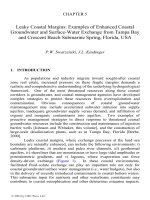
Figure 1: Fresh groundwater flow and discharge pattern
(after Glover [1964]).
data collection and analysis, have encouraged the study of the dynamic
aspects of tidal effects for coastal groundwater seepage analysis [Gilbin and
Gaines, 1990; Millham and Howes, 1994; Portnoy et al., 1998].
The objective of this discussion is to describe the dynamic concept
of the coastal freshwater–saltwater relationship and the techniques that can
be used to determine coastal fresh groundwater seepage in a quantitative and
qualitative form. The descriptions and methods described are primarily
directed to the more quiescent shores of the relatively sheltered bays and
lagoons, and generally the source of most critical environmental concerns. It
is further most applicable to the sandy seashore, influenced by the changing
water levels of the ocean tides. In many cases a sandy beach or cove, even on
the rock bound coast, is the zone of primary fresh groundwater discharge.
2. CONCEPTS
2.1 Freshwater-Saltwater Relationships
Where freshwater meets saltwater in a permeable landmass, the
freshwater will tend to float on the more dense saltwater according to the
Ghyben-Herzberg Principle [Drabbe and Ghyben, 1889; Herzberg, 1901]. In
© 2004 by CRC Press LLC
Beach Face Seepage
145

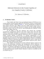
Figure 2: The sequence of coastal groundwater discharge through a sandy
beach during the tidal cycle.
an insular landmass, such as an island or peninsula, this configuration of
body of freshwater will approximate a lens, bounded by and underlain by
saltwater. The coastal manifestation of this lens is a pinching out of the lens
at the coastal boundary to discharge through a narrow zone at the tidal
margin described in a steady state theoretical case by Glover [1964], and as
further illustrated for a coastal margin in Figure 1.
Delineation of coastal discharge is a much more elusive problem
when one considers the changing groundwater conditions in the inter-tidal
zone incorporating the complexities of a boundary which changes cyclically
twice a day both laterally and vertically, highly variable salinity, fluctuating
hydraulic heads, and a geologically heterogeneous beach [Turner, 1993a;
Baird and Horn, 1996; Robinson and Gallagher, 1999; Li et al., 2000].
2.2 The Moving Boundary
In tidally influenced coastlines both the freshwater lens and the
discharge patterns are greatly changed from a static condition, depending on
the topography and geologic nature of the beach inter-tidal zone. The water
table in the coastal groundwater moves up and down with the tide;
concurrently the boundary on a sloping beach surges shoreward and seaward;
the beach is flooded with saltwater twice a day, and in many cases the
hydraulic discharge gradient itself changes direction, an extremely complex
and dynamic situation. The basic process of coastal groundwater discharge
© 2004 by CRC Press LLC
Coastal Aquifer Management
146
through an idealized homogeneous sandy beach during a tidal cycle is
illustrated in Figure 2.
During high tide, groundwater flow is hydraulically blocked, with a
reverse hydraulic gradient toward the land imposed by the tide, which is

higher than the near-shore water table; additionally, saltwater will infiltrate
into the land surface adding to and mixing with the fresh groundwater in the
beach.
As the tide ebbs the hydraulic gradient reverses and groundwater
flow consisting of both salt and freshwater moves toward the lower beach.
As low tide approaches groundwater discharge occurs, both as beach face
seepage and lower beach submarine discharge. With the rising tide a reverse
hydraulic gradient is again established and the groundwater discharge ceases.
The cycle then repeats.
Field sampling of coastal groundwater discharge is greatly
complicated by the transient nature of the tidally induced changing boundary.
The timing and location of the quality of groundwater in three dimensions
becomes critical for groundwater sampling. This is further complicated by
the indistinct and changing salinity of the beach groundwater and discharge.
The earliest freshwater lens models made no attempt to discretely character
the hydraulic and chemical nature of the seepage, treating it as a fixed sharp
line in time and space.
A significant advancement was the theoretical formulation of the
discharge gap representation to describe coastal seepage by Glover [1959]
and further described by Cooper [1965] under steady state conditions. This,
however, failed to take into account anything other than the assumed
discharge without regard for the salinity of the discharge. The distribution of
the discharge as a decreasing exponential pattern was first examined in a
field setting on the shores of Long Island by Bokuniewicz [1980, 1992],
referencing earlier freshwater lake seepage studies by McBride and
Pfannkuch [1975]. These field observations, however, were under essentially
tideless conditions.
Because of the laterally moving boundary on a sloping beach, there
is a much wider outflow gap as well as major changes in the flow pattern of
the discharge, including in many cases a complete reversal of flow and

salinity. A beach face model, SEEP, was developed by Turner [1993a] to
analyze and predict the exit dynamics of groundwater seepage with a falling
tide. Turner further describes the role of the capillary fringe in the total water
content of the beach.
2.3 Beach Slope Effect
While the determination of mean sea level (MSL) in the open coastal
water system is a necessary base line, it should be recognized that in a
© 2004 by CRC Press LLC
Beach Face Seepage
147
sloping beach there is a dynamic phenomenon caused by the tide movement
which can create an “effective mean sea level” (EMSL) in the beach
considerably above open water measured MSL [Urish and Ozbilgin, 1989].
This was later elaborated on by Nielsen [1990] and Hegge and Masselink
[1991]. The seawater is mounded in the upper beach by the dynamic
movement of tide and consequent infiltration of saltwater as it moves up the
beach face. There is, in effect, a pumping action caused by rapid infiltration
of the seawater in the upper beach during high tide and much slower
drainage of the seawater through the lower beach at low tide. This results in a
super elevation of the apparent sea level boundary condition, which has been
measured as much as 0.5 feet above open water MSL for a 5 foot tide range
on a 0.05 beach slope [Urish, 1980]. This becomes important in modeling
coastal boundary conditions.
The inter-tidal beach is subjected to seawater flooding and
infiltration from the rising tide, which is then a substantial component of the
beach discharge. The rising edge of the incoming tide advances shoreward
faster than the discharging freshwater can rise. Thus, the seawater quickly
fills the available pore space in the sands of the upper beach, sometimes
rising rapidly enough to trap air under the surface. The quantity of infiltrated
saltwater in the beach which becomes seepage depends on the residual water

content from the previous saturation episode, as well as the downward
directed hydraulic gradient. The residual water in the upper portion of the
inter-tidal zone is usually a layered mixture of saltwater over freshwater with
some mixing, depending on the magnitude of the freshwater discharge and
the antecedent drainage characteristics of the beach.
As Bokuniewicz [1992] points out, however, saline pore water
overlying fresh pore water has an inherently unstable density gradient,
causing “fingering” of the different densities of water to occur; this leads to
greater uncertainty in any attempts at determining the volume of infiltrated
saltwater directly. The presence, however, of a substantial layer of infiltrated
saltwater overlying freshwater in the inter-tidal zone is well established by
both direct water table sampling [Portnoy et al., 1998] and by indirect
surface electrical resistivity soundings in the inter-tidal beach [Frohlich,
2001].
3. METHODOLOGY
3.1 Elevation Measurements
3.1.1 Elevation Control and Datums
In order to relate water levels to the beach and near-shore surfaces it
is essential that beach topographic profiles be made and referenced to a fixed
© 2004 by CRC Press LLC
Coastal Aquifer Management
148
datum, the same as used for setting elevation reference points on monitor
wells and tidal stations in the study area. While more sophisticated (and
expensive) survey methods such as the “total station” may be used, for the
limited area usually involved, the “automatic level” and tape are generally
most efficient. The most frequently used reference datum is the 1929
National Geodetic Vertical Datum (NGVD29) or more recent North
American Vertical Datum of 1988 (NAVD88), which can be related for a
specific geographic area to the NGVD29 by an adjustment constant. While

the NGVD29 datum is frequently referred to as “mean sea level”, it is only a
very crude approximation, and is far from the precision necessary for coastal
water level measurements.
Complicating coastal elevation measurements is the fact that tide
table predictions and tide station measurements are usually reference to
locally determined assigned datums of mean lower low water (MLLW). This
is a datum determined as zero from the average of the lower of the two low
waters of each day for the past 19 years. For the United States the values in
popular references such as Reed’s Nautical Almanacs [Herzog, 2003] are
still in feet, rather than the more globally accepted meters. Tide level
predictions for specific locations can also be obtained from the National
Oceanic and Atmospheric Administration (NOAA) web site www.co-
ops.nos.noaa.gov [Wolf and Ghilani, 2002]. The correction necessary to
convert the local MLLW value to a 1929 NGVD or 1988 datum can be
obtained from the web site. For example, for the Narragansett Bay 2.92 feet
must be subtracted from the MLLW value of tide to obtain the equivalent
water level relative to the NGVD 1929 Datum. This is necessary information
for coastal field investigation planning and coastal engineering.
3.1.2 Water Level Measurements
Water level measurements taken to a precision of 0.03 m and
referenced to a datum are essential to any study of groundwater in order to
evaluate the transport and movement characteristics of the groundwater, the
receiving water, and tidal systems. These water level measurements are
generally used as direct measurements of hydraulic heads and piezometric
pressures.
Any number of water level measurement (depth to water) techniques
can be used depending on the length of time of the investigation, the
precision required and the resources available. The following discussion is
divided into the general categories of short term and long term. It is intended
to be comprehensive, but is most specifically not inclusive of all possible

techniques.
In all cases it is important to recognize the importance of
concurrently determining the density of the water in the monitor wells being
© 2004 by CRC Press LLC
Beach Face Seepage
149
measured, usually determined indirectly as a function of measured salinity.
The concept of variable water density as it relates to groundwater flow
systems is explained in excellent detail by Lusczynski [1961]. All water
level measurements must be converted to freshwater or saltwater equivalents
in order to evaluate the water levels as hydraulic heads. To make this
conversion both the depth of the water column in the monitor well as well as
the salinity (density) must be known. As an example, the measured water
level in a monitor well with a column of 3.00 m of saltwater with a density of
1.020 must be increased by 0.06 m to be a freshwater equivalent for
comparison with the heads in freshwater monitor wells.
3.1.2.1 Short-term water level measurements
Manual point-in-time depth to water measurements can be
accomplished in monitor well or tidal stilling wells by several methods. Once
the depth to water is determined from the top of a well casing with known
elevation referenced to a datum, subtraction of that value from the well
casing elevation gives the water level elevation. This can be done by direct
water level measurement with a tape in shallow wells and by the “wetted
tape” method or with electrical response devices in deeper wells.
3.1.2.2 Long-term water level measurements
In many cases the field study requires a long-term continuous series
of measurements, which may extend into months. In other cases it is
necessary to collect data from many wells simultaneously and at very short
intervals of time. For such cases it is not feasible, if not impossible, to collect
data points manually. For this purpose mechanized or computerized data

collection is necessary:
A) The oldest method is the drum water level recorder in which a float is
connected mechanically to a time oriented rotating drum. A pen in the
recorder then traces the track of water fluctuation on graph paper placed
on the rotating drum. As might be expected there are many opportunities
for recorder failure; among other things, the pen may run out of ink, the
power source may run out, the float may get fouled, etc. The benefit is
that with well-maintained equipment and frequent performance checks it
gives a direct visual plot of results. The graphic plot then must be
manually converted to digital values for further analysis.
B) The most commonly used method is the hydraulic pressure transducer.
This consists of a computer data logger connected by cable to a small
diameter pressure transducer probe that can be placed in the well. The
probe measures the water level by the pressure changes on a very small
diaphragm that then transmits electrical signals of its movement to the
© 2004 by CRC Press LLC
Coastal Aquifer Management
150
data logger. The water level is actually measured as the weight of water
above a carefully elevation-referenced transducer. It is apparent then that
the calibration of the transducer must be corrected for the density of
water; e.g., if a transducer calibrated for freshwater use is placed under
4.00 m of sea water at a density of 1.025, rather than freshwater at a
density of 1.000, then the logger reading will be 4.10 m rather than 4.00
m, a very significant difference in groundwater measurements. The
logger unit can be programmed for timing and frequency of data
collection and downloaded directly into a computer file.
C) A more recent automatic water level recorder especially suitable for
shallow systems is the “Ecotone” capacitance water level monitoring
instrument, manufactured by Remote Data Systems, which uses an

electrical wire capacitor method. This requires a special tube or monitor
well and so is not as adaptable as the pressure transducer, which can be
placed in any well, but does have the advantage that each well is a self-
contained unit and so can be placed in widely separated remote locations.
Further, it is not affected by water density and barometric pressure. As
with the pressure transducer logger, it can be programmed for frequency
interval of data collection and downloaded directly into a computer file.
3.2 Beach Sediments and Topography
Recognizing that the hydraulic conductivity of beach sediments may
vary greatly both horizontally and vertically, it is very useful to take soil
samples at different locations along the beach to characterize the beach and
its variability. Undisturbed samples should be collected during low tide in
tubes pressed into the walls and bottoms of excavations to obtain both
horizontal and vertical oriented samples. If a disturbed sample is all that can
be obtained, then care should be taken to compact it to a maximum density to
approximate the in-situ condition before running permeability tests. In this
case it should be recognized that the inherent in-situ anisotropy, which may
range from 5 to 50 for beach samples, is lost in the reconstituted sample. It is
possible to assume a value for anisotropy and back calculate probable values
for K
h
and K
v
using the relationship
1/ 2
()
hv
KKK= . If a reasonable value of
10 is taken, then K
h

= 3.16 K and K
v
= K/3.16.
It is necessary to determine the beach profile to understand the
relationship of measured water table and tide levels to the beach surface
through which seepage occurs. The profile should be referenced with
horizontal and vertical control in order that subsequent beach surveys can be
related to the same fixed reference. Beach surfaces are far from stable,
changing with each tidal cycle and more dramatically with storms. For long-
term studies a number of profiles need to be accomplished.
© 2004 by CRC Press LLC
Beach Face Seepage
151
3.3 Coastal Seepage Measurements
3.3.1 Thermal Infrared Aerial Imagery
Thermal infrared imagery has been a particularly useful tool to
determine coastal fresh groundwater discharge patterns and specific
locations. The proper application of the technique, however, requires careful
attention to the timing of coastal groundwater discharge. In a beach
composed of permeable porous media the timing of the imaging survey must
occur during the period ½ hour before to 1 hour after low tide, during the
period of maximum fresh groundwater discharge. It should be noted,
however, that there are some hydrogeologic exceptions to this general rule,
namely in coastal environments where a beach confining or semi-confining
layer may preclude open phreatic discharge through the beach. In such a case
the water table will be elevated by a rising tide and discharge may take place
at high tide in the upper beach at the upper limit of the confining layer; only
a detailed on-site survey can ascertain if such a hydrogeologic condition
exists in the areas of interest.
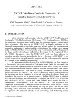
The thermal infrared method maps temperatures of surfaces exposed

to a super-cooled detector, which is mounted on a small aircraft. The results
can be visually interpreted to identify groundwater discharge along a coastal
margin by measuring the difference in thermal spectral response of the water
along the coast. The temperature contrast can be either a colder groundwater
to warmer receiving water as occurs in the late summer or warmer
groundwater to colder receiving water as occurs in the winter months. For a
successful thermal imagery survey the groundwater-receiving water
temperature contrast should be no less than about 5
±C. The ability to detect
the colder groundwater is further enhanced by the tendency of the less dense
freshwater to float on the top of saltwater. In a summer survey the colder
fresh groundwater appears as a dark plume emanating from the shore. There
should be two flight runs accomplished approximately ½ to 1 hour apart in
order to distinguish between fixed coastal features, which also may give a
thermal response, and the moving plumes of discharging freshwater. This is
illustrated in Figures 3 and 4, which show images of a moving freshwater
plume taken one hour apart during low tide.
3.3.2 Beach Salinity Transects
Beach salinity sampling transects can be made transverse and
parallel to the beach line at low tide to ascertain the variability of quality of
seepage in a local zone. Such sampling must be at closely spaced locations,
but because the quality and location of the water changes with time it is
necessary that the sampling be done very rapidly. This is best done by

© 2004 by CRC Press LLC
Coastal Aquifer Management
152

Figure 3: Thermal infrared image of fresh groundwater plume (image one).
extracting small water samples at shallow depths with a small probe attached

to a manually operated syringe. The small quantity thus obtained can then be
rapidly analyzed for salinity using a small handheld refractometer.
3.3.3 Direct Beach and Coastline Water Quality Sampling
The selection of a proper method for groundwater sampling in the
beach environment depends on the intent and duration of the survey, and
implicitly the available resources. It is important to recognize that all direct
sampling methods are point measurements and hence may not be
representative of seepage over a broader regional shoreline because of the
great heterogeneity of the coastal discharge zone. Field measurements of
piezometric heads as well as low tide beach observations indicate that a
substantial amount of discharge occurs under both subaerial and submarine
conditions. An additional consideration is that single point sampling may be
completely out of a primary freshwater seepage zone even though substantial
discharge may occur. Thus one should consider a broader based

© 2004 by CRC Press LLC
Beach Face Seepage
153

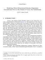
Figure 4: Thermal infrared image of freshwater plume (image two), 1 hour
after that of Figure 3.
reconnaissance such as the thermal infrared imagery, or at least rapid
shoreline transects, to identify zones of probable fresh groundwater
discharge before detailed sampling is undertaken.
3.3.3.1 Short-term sampling
Short-term sampling to characterize the nature of coastal
groundwater in three dimensions can be done by direct sampling with probes
and by seepage meters. Discrete groundwater sampling can be done both
rapidly by shallow probes going only a few centimeters into the seepage
face, by deeper hand-driven probes going as deep as 5 m, or even deeper by

power procedures.
In the submarine part of the discharge zone seepage meters can be
used. Seepage meters are limited to sampling for submarine seepage since
they must remain under water. While more sophisticated electronic devices
are now coming on the market, most seepage meters have two basic
components, namely, a shallow pan usually no larger than a meter which is
© 2004 by CRC Press LLC
Coastal Aquifer Management
154
inverted over the area to be sampled, and a seepage bag placed on a stopcock
set in the inverted pan [Lee, 1977]. The seepage water then flows through the
confined space of the inverted pan and accumulates in the bag. The amount
of water collected over a determined period of time can then be measured
and seepage rate calculated. More recent innovations of the seepage meter
have been made to accomplish automated continuous flow measurements
3.3.3.2 Long-term sampling
Long-term sampling at fixed locations is best done utilizing properly
installed monitor wells for both water quality and water level measurements.
While good monitor wells can be installed by hand methods, it is frequently
more expedient to contract a well driller, preferably from a geotechnical firm
familiar with the purpose and technical specifications for monitor wells. The
best drilling method employs the hollow stem auger which permits the
obtaining of relatively undisturbed split spoon samples as well as water
samples at specific depths during the drilling process. In order to ascertain
the vertical distribution of water quality and piezometric heads a nest of at
least three monitor wells needs to be installed at each location.
3.3.4 Water Quality Measurements
The primary parameters of interest in field measurement to locate
coastal fresh groundwater seepage are electrical conductivity, salinity, and
temperature. After the best sampling locations are ascertained, additional

conventional field measurements such as pH and oxygen can be taken, and
samples collected, preserved, and conveyed to a laboratory for chemical
analysis to any degree of sophistication desired.
The best all around instrument for the exploration phase of seepage
investigation is the YSI temperature-conductivity-salinity meter. This is
rugged and versatile, and while limited in precision relative to fixed
laboratory instruments, is quite suitable for ascertaining if seepage water is
fresh or salty. The refractometer is a very convenient instrument for rapid
measurements of limited precision; this can determine salinity only to ppt,
but can provide a reading very rapidly and requires only a drop of water.
4. CASE STUDY [URISH AND QANBAR, 1997]
4.1 Study Location
The study was conducted along the beaches of the Nauset Marsh
embayment (Figure 5), a 945 ha back-barrier estuary on Cape Cod, MA
connected by an inlet to the Atlantic Ocean.
© 2004 by CRC Press LLC
Beach Face Seepage
155

Figure 5: Study location for coastal fresh groundwater seepage.
The surficial deposits are largely unconsolidated glacial sediments
deposited by glacial ice and melt water at the close of the Wisconsin
Glaciation, some 10,000 years ago. Very old granitic bedrock lies about 170
m below the surface. The beaches are composed of marine reworked
shoreline deposits, predominantly of relatively uniform quartz composition
ranging from silt to coarse sands. The Nauset Marsh embayment is
dominantly medium to coarse sands, with thin upper layers of silt at some
locations. In the beaches investigated there was a median grain size diameter
range of 0.40 to 1.00 mm and a D
10

size (“effective size”) of 0.10 to 0.36
mm.
The topography of the study area is undulating with elevations
ranging from sea level to 4.25 m. There are numerous bays, coves, and
coastal wetlands. Surface streams are infrequent with much of the
precipitation infiltrating into the sandy soil. The climate of the region is a

© 2004 by CRC Press LLC
Coastal Aquifer Management
156

Figure 6: Profile of beach face showing location of monitoring wells and
seepage during a tidal cycle.
maritime humid temperate climate. The average annual rainfall of 110 cm is
evenly distributed throughout the seasons. The aquifers are phreatic with the
groundwater occurring as a freshwater lens “floating” on the denser
underlying salt water. The Nauset Marsh complex is a shallow marine
environment with tides in the 1- to 2-m range, averaging about 1.34 m.
Salinity in the central parts of the water bodies is near that of the connecting
Atlantic Ocean, in the range of 25 to 30 ppt; the near-shore salinities are less,
being strongly influenced by the discharging freshwater, particularly during
low tide periods.
4.2 Methodology
Sets of monitor wells consisting of 3.2 cm inside diameter PVC pipe
with 7.6 cm screen at the lower ends were installed in the beach zone for
piezometric measurements and water quality sampling as shown in Figure 6.
These were placed by hand augering with the center of the screens set 45 cm
below the beach face and below the lowest position of the water table. Water
levels were measured both by direct tape measurements and by pressure
transducers placed in the monitor wells, as well as in the open water for tidal

measurements. Hydraulic head values were corrected for density variation to
freshwater equivalent heads as appropriate [Kohout, 1961; Lusczynski,
1961].
© 2004 by CRC Press LLC
Beach Face Seepage
157

Figure 7: Plot of tide and groundwater levels under low tide conditions.
Low tide shoreline reconnaissance sampling for groundwater
discharge salinity was accomplished using a 2 mm internal diameter stainless
steel probe with a fine screen tip pushed about 10 cm into the sediments, and
the water drawn by vacuum into a syringe set on the tube’s upper end.
Salinity was determined using a handheld refractometer in the field and by
YSI instrument in the lab for collected water samples. Values were
standardized to 25°C. Soil samples were also taken in seepage areas and
analyzed for grain size using sieve analysis and hydraulic conductivity by the
falling head permeameter test, both by ASTM Standards.
The elevations of all monitor wells were established by standard
leveling techniques using a TOPCON automatic level and referenced to 1929
National Geodetic Vertical Datum (NGVD), or to an arbitrary local datum
where a NGVD benchmark was not available.
4.2.1 Infiltration and Seepage Mechanism
In order to examine the seepage dynamics in detail during a tidal
cycle field studies were made at two sandy beach sites in the Nauset Marsh
estuary complex. Monitor well water level measurements in the beach for the
low tide phase (Figure 7) illustrate the relationships between beach
groundwater and tidal water during low and high tide episodes. Groundwater
piezometric head measurements at one monitor well at the low tide line and
surface water elevations were monitored at 15-min intervals for 7 days using
© 2004 by CRC Press LLC

Coastal Aquifer Management
158
pressure transducers attached to automatic data loggers. Using this
information, episodes of high and low tide were selected for detailed seepage
analysis.
Results show that for saltwater infiltration to occur two conditions
need to exist, namely, 1) The saltwater level in the open water must be
higher than the ground surface elevation that it floods, and 2) The saltwater
level has to be higher than the groundwater hydraulic head at the monitor
well location in the flooded beach. In this case the analysis must examine
both subaerial and submarine hydraulic conditions in the beach as the tide
recedes past the monitor well location. It is observed that at 21.0 hours
infiltration is still occurring, but beginning at 21.6 hours the groundwater
head becomes higher than the tide water, but both are higher than the beach
surface, thus underwater seepage occurs. At about 22.5 hours the tide level
falls below the beach surface at the monitor well, but since the piezometric
head of groundwater is greater than the beach surface elevation, surface
seepage exists. This continues until 23.2 hours when the beach location is
again flooded by a rising tide and submarine seepage occurs. At 23.6 hours
seepage ceases and infiltration begins again.
4.2.2 Temporal and Spatial Pattern of Seepage
Using the analytical process described in the preceding section for
one monitor well location on the beach, full beach seepage analysis at three
sites was accomplished using sets of monitor wells installed transverse to the
beach.
A time sequence of plots (Figure 8) showing the magnitude of net
hydraulic heads along the beach face over the lower part of the tidal cycle
provides insight into the temporal and spatial pattern of seepage as the tide
moves down and back up the beach face.
The shaded areas under the curve denote submarine seepage where

the tide covers the beach. The sequence starts with all locations showing
submarine seepage at 9.0 hours; there was no seepage at 8.0 hours. It is to be
noted that the location and magnitude of greatest seepage changes with time,
generally moving seaward with the tide. Finally, the sequence ends with all
locations showing infiltration.
When the time sequence of seepage is recalculated as average
seepage during the tidal cycle, the result of seepage distribution relative to
the beach face is as shown in the bottom part of Figure 6. The seepage
indicated is composed of both fresh groundwater and infiltrated saltwater.
© 2004 by CRC Press LLC
Beach Face Seepage
159

Figure 8: Temporal and spatial sequence of beach seepage and infiltration.
© 2004 by CRC Press LLC
Coastal Aquifer Management
160
4.2.3 Quality of Seepage
The salinity of the seepage varies with location and time. The
freshest measured discharge was 2 ppt, which occurred during low tide at the
location of maximum seepage, while the highest salinity of 30 ppt was at the
beginning of the discharge period. At all sites the lower part of the seepage
zone displayed minimum salinity especially during the lowest part of the
tidal cycle. The early discharge includes considerable flushing of saltwater
which infiltrated into the beach during the flooding tide.
It seems apparent that the infiltrated saltwater is a major part of the
shoreline seepage, which can vary widely, depending on the climatic
conditions which enable fresh groundwater discharge, but perhaps more
importantly on the beach face geometry and the magnitude of tide. While
there is wide variability in estimates of fresh and saltwater discharge by the

various approaches, it does indicate that a large proportion of beach
discharge is infiltrated saltwater, probably in the range of 65–85% for the
sites studied. In arid region coastlines it may be much higher, and in wetter
coastal areas, much lower. The distribution of subaerial and submarine
seepage is more dependent on the beach characteristics of slope, hydraulic
conductivity, and tidal range [Turner, 1995]. For Site A about 55% of the
seepage is submarine seepage, but for Site B, only 35% is submarine
seepage.
4.2.4 Shoreline Seepage Variability
In order to evaluate the physical evidence for variability of seepage
along the beach front, soil samples were taken at both visually apparent high
seepage zones and those that exhibited less seepage. It was found that the
average median grain size for soil was 1.50 mm in the high seepage areas
and 0.070 mm in the low seepage areas. It appears that once seepage is
initiated it is self-enhancing by washing out the fines and creating higher
hydraulic conductivity. Confirmation of this was established by employing
Hazen’s equation for hydraulic conductivity at the two zones which gave
values of 78 m/day and 20 m/day for the high and low seepage zones,
respectively. Airborne thermal infrared imagery was also used to ascertain
the shoreline fresh groundwater discharge. This method is able to depict the
freshwater discharge by imaging the temperature difference using spectral
wave length differences between discharging fresh groundwater and the
warmer receiving sea water [Portnoy et al., 1998] in the late summer.
As shown in Figure 9, for one of the study sites at Nauset Marsh, the
freshwater discharge is shown as dark plumes emanating from the shoreline.
Additionally, direct water quality measurements during low tide discharge at
the site provided ground-truthing of the variation in shoreline salinity, as

© 2004 by CRC Press LLC
Beach Face Seepage

161

Figure 9: Thermal infrared imagery at Town Cove, Nauset Marsh.
illustrated in Figure 10. Dramatic indications of the shoreline variation in the
salinity of discharge is evident, as well as the relationship of salinity with
nitrogen, a selected chemical sampling parameter.
© 2004 by CRC Press LLC
Coastal Aquifer Management
162

Figure 10: Shoreline discharge salinity and nitrogen distribution at low tide.
5. SUMMARY
The nature of coastal groundwater seepage when viewed in the
dynamic temporal and spatial context is highly complex, necessitating the
use of many different methods and tools. It is best to begin with a broader
© 2004 by CRC Press LLC
Beach Face Seepage
163
based survey, such as the thermal infrared imagery or rapid shoreline salinity
transects which will identify regions of fresh groundwater discharge. Then
more focused attention can be effectively given to more detailed short-term
and long-term sampling.
Acknowledgments
The information contained in the foregoing discussion is largely
based on island and coastal groundwater studies funded by the National
Science Foundation, Sea Grant, and the National Park Service. The support
of these agencies is gratefully acknowledged as well as that of the many
colleagues and graduate students who participated in the fieldwork.
REFERENCES
Baird, A.J. and Horn, D.P., “Monitoring and modeling groundwater

behaviour in sand beaches”, Journal of Coastal Research,
12(3),
630–640, 1996.
Barwell, V.K. and Lee, D.R., “Determination of horizontal to vertical
hydraulic conductivity ratios from seepage measurements on lake
beds”, Water Resources Research,
17(3), 565–570, 1981.
Bokuniewicz, H., “Groundwater seepage into Great South Bay, New York”,
Estuarine and Coastal Marine Science,
10(4), 437–444, 1980.
Bokuniewicz, H. and Pavlik, B., “Groundwater seepage along a barrier
island”, Biogeochemistry, 1990.
Bokuniewicz, H., “Analytical descriptions of subaqueous groundwater
seepage”, Estuaries,
15(4), 458–464, 1992.
Cooper, H.H., Jr., Kohout, F.A., Henry, H.R., and Glover, R.E., “Sea water
in coastal aquifers”, U.S. Geological Survey Water-Supply Paper
1613-C, Washington, D.C., 82 p., 1964.
Drabbe, J. and Badon Ghijben, W., “Nota in verband met de voorgenomen
putboring nabij,” Amsterdam. Tsch. Kon. Inst. v. Ingenieurs, Verh.
1888–1889, The Hague. 8–22, 1889.
Frohlich, R.K., “Vertical electrical resistivity soundings in a Provincetown
beach”, personal communication, April, 2002.
Giblin, A.E. and Gaines A.G., “Nitrogen inputs to a marine embayment: the
importance of groundwater”, Biogeochemistry,
10, 309–328, 1990.
Glover, R.E., “The pattern of fresh water flow in a coastal aquifer”, Journal
of Geophysical Research,
64(4), 457–459, 1959.
Glover, R.E., “The Pattern of fresh water flow in a coastal aquifer”, U. S.

Geological Survey Water Supply Paper 1613C:C32–C35, 1964.
© 2004 by CRC Press LLC
Coastal Aquifer Management
164
Hegge, B.J. and Masselink, G., “Groundwater-table responses to wave run-
up: an experimental study from Western Australia,” Journal of
Coastal Research,
7(3), 623–634, 1991.
Henry, H.R., “Interfaces between salt water and fresh water in coastal
aquifers”, U.S. Geological Survey Water Supply Paper 1613C: C35–
C70, 1994.
Herzog, C., Reed’s Nautical Almanac, North American East Coast, Thomas
Reed Publications, Providence, RI, 2003.
Herzsberg, A., “Die Wasserversorgung,” Jahrb. Jahrg.,
44, Munich. 815–
819, 842–844, 1901.
Hubbert, M.K., “ The theory of groundwater motion”, Jour. Geology,
48, no.
8, pt. 1, 785–944, 1940.
Kohout, F.A., “Fluctuations of ground-water levels caused by dispersion of
salts”, Journal of Geophysical Research,
66(8), 2424–2434, 1961.
Lee, D.R., “A device for measuring seepage flux in lakes and estuaries”,
Limnology and Oceanography,
22, 140–147, 1977.
Li, L., Barry, D.A., Stagnetti, F., Parlange, J.Y., Jeng, D.S., “Beach water
table fluctuations due to spring-neap tides: moving boundary
effects”, Advances in Water Resources,
23, 817–824, 2000.
Lusczynski, N.J., “Head and flow of ground water of variable density”,

Journal of Geophysical Research,
66(12), 4247–4256, 1961.
McBride, M.S. and Pfannkuch, H.O., “The distribution of seepage within
lake beds”, Journal Research, U.S. Geological Survey 3, no. 5: 505–
512, 1975.
Millham, N.P. and Howes, B.L., “Nutrient balance of a shallow coastal
embayment: I. Patterns of groundwater discharge”, Marine Ecology
Progress Series 112, 155–167, 1964.
Nielsen, P., “Wave setup: a field study”, Journal of Geophysical Research,
93(C12), 15643–15652, 1988.
Nielsen, P., “Tidal dynamics of the water table in beaches”, Water Resources
Research,
26(9), 2127–2134, 1990.
Portnoy, J.W., Nowicki, B.L., Roman, C.T., and Urish, D.W., “The
discharge of nitrate-contaminated groundwater from developed
shoreline to marsh-fringed estuary”, Water Resources Research,
34(11), 3095–3104, 1988.
Robinson, M.A. and Gallagher, D.L., “A model of groundwater discharge
from an unconfined aquifer”, Ground Water,
37(1), 80–87, 1999.
Turner, I., “Water outcropping on macro-tidal beaches: a simulation model”,
Marine Geology,
115, 227–238, 1993a.
Turner, I., “The Total Water Content of Sandy Beaches”, Journal of Coastal
Research,
S1, no. 15, 11–26, 1993b.
© 2004 by CRC Press LLC
Beach Face Seepage
165
Turner, I., “Simulating the influence of groundwater seepage on sediment

transported by the sweep of the swash zone across micro-tidal
beaches”, Marine Geology,
125, 153–174, 1995.
Urish, D.W., “Asymmetric variation of Ghyben-Herzberg lens”, Jour. Hydr.
Div. Proc. American Society of Civil Engineers,
107, 1149–1158,
1980.
Urish, D.W., “The Effect of Beach Slope on the Fresh Water Lens in Small
Oceanic Landmasses”, Technical Completion Report, National
Science Foundation Grant No. Eng-7908084, 1982.
Urish, D.W. and Ozbilgin, M., “The Coastal Ground-Water Boundary”,
Ground Water,
26, 267–289, 1989.
Urish, D.W. and Qanbar, E., “Hydrologic Evaluation of Groundwater
Discharge at Nauset Marsh, Cape Cod National Seashore,
Massachusetts”, Technical Report NPS/NESO-RNR/NRTR/97-07,
1997.
© 2004 by CRC Press LLC