Environmental Fluid Mechanics - Chapter 3 docx
Bạn đang xem bản rút gọn của tài liệu. Xem và tải ngay bản đầy đủ của tài liệu tại đây (673.38 KB, 38 trang )
3
Viscous Flows
3.1 VARIOUS FORMS OF THE EQUATIONS OF MOTION
Viscous flows are mathematically represented by solutions of the equations
of motion, based on momentum transfer in an elementary fluid volume. The
equations of motion for viscous flows are the Navier–Stokes equations intro-
duced in the previous chapter. For convenience, we repeat these equations
here, for cases in which variations in viscosity are negligible:
∂
E
V
∂t
C
E
V Ðr
E
V D
1
rp C gZ C
vr
2
E
V3.1.1a
where V is the velocity, t is time, r is the gradient vector, is the density, p
is the pressure, g is gravitational acceleration, Z is the elevation with regard
to an arbitrary reference, and
v is the kinematic viscosity. In Appendix 1,
tables of Navier–Stokes equations for Cartesian, cylindrical, and spherical
coordinate systems are listed. In Appendix 2, relationships are given between
stress components and velocity components, as implied by the Navier–Stokes
equations.
Using Cartesian tensor notation, Eq. (3.1.1a) is represented as
∂u
i
∂t
C u
k
∂u
i
∂x
k
D
1
∂p
∂x
i
g
∂Z
∂x
i
C v
∂
2
u
i
∂x
2
k
3.1.1b
where u
i
represents components of the velocity vector and x
i
represents
the coordinates. This equation incorporates four unknown quantities: three
components of the velocity vector and the pressure. Along with the continuity
equation, we thus have a system of four differential equations with four
unknowns. The solution of this system subject to appropriate initial and
boundary conditions provides the required information about the distribution
of the unknown quantities in the domain.
The distributions of velocities and pressure depend on the three space
coordinates, x, y and z, and the time coordinate, t. It should be noted that the
Copyright 2001 by Marcel Dekker, Inc. All Rights Reserved.
order of the differential equation (3.1.1) varies with regard to the unknown
quantities, as well as with regard to the various coordinates. The velocity
components contribute terms of first order with regard to time and of both
first and second order with regard to the space coordinates. The pressure
contributes terms of first order with regard to the space coordinates. The order
of the partial derivatives indicates the number of boundary conditions needed
for the solution of this system of partial differential equations. The pressure
should be given at a certain point in the domain during all times. The velocity
distribution at initial conditions should be given for the whole domain. The
velocity at a sufficient number of boundaries should be given for the required
time period of the simulation. There are several typical boundary conditions
for the velocity vector, or its derivatives. The latter are related to shear stresses.
Generally, there are four typical boundary conditions for the velocity and the
shear stresses:
Boundary between the viscous fluid and a solid boundary — fluid
velocity is identical to that of the solid boundary, as the viscous fluid
adheres to the solid boundary.
Boundary between two viscous immiscible fluids — velocity and shear
stress at both sides of the interface are identical.
Boundary between two immiscible fluids with an extremely large differ-
ence of viscosity, e.g., liquid and gas — shear stress vanishes at
the interface between the two fluids. (An exception to this rule is
with wind-driven flows, where boundary shear stress is significant.
Momentum transfer at the air/water interface is discussed in Chap. 12,
and a particular application, in a geophysical context, is discussed in
Chap. 9.)
Finite domain — the velocity has finite value at every point of the
domain.
As viscous fluid flow is basically a rotational flow, the equation of
motion (3.1.1) can be represented as an equation of vorticity transport. The
rotationality of the flow is represented by the distribution and intensity of the
vorticity. The vorticity is a kinematic tensorial characteristic of the flow field.
The tensor of vorticity is a second-order asymmetric tensor. Such a tensor
has three pairs of components. Each pair incorporates two components of
identical absolute value and opposite sign. Therefore the vorticity also can be
represented by a vector with three components. Each component of this vector
represents one pair of components of the vorticity tensor. By the employment
of Cartesian tensor notation, the vorticity vector is defined as
ω
j
D
∂u
i
∂x
k
∂u
k
∂x
i
3.1.2
Copyright 2001 by Marcel Dekker, Inc. All Rights Reserved.
where i, j, k D 1, 2, 3. One half of the vorticity represents the angular rotation
rate of an elementary fluid volume, as previously noted.
By cross differentiation and subtraction of component equations of
Eq. (3.1.1b), the pressure is eliminated from the equation of motion. Then
the expression of Eq. (3.1.2) can be introduced to obtain a vorticity equation,
Dω
j
Dt
ω
k
∂u
j
∂x
k
D v
∂
2
ω
j
∂x
2
k
3.1.3
where
Dω
j
Dt
D
∂ω
j
∂t
C u
k
∂ω
j
∂x
k
3.1.4
The first term on the LHS of Eq. (3.1.3) represents the total rate of change of
vorticity. The second term represents the deformation of a vortex tube. The
term on the RHS of Eq. (3.1.3) represents the diffusion of vorticity due to the
viscosity of the fluid.
In cases of two-dimensional flow the vorticity vector has a single compo-
nent, and the term representing the deformation of the vortex tube vanishes.
Then, Eq. (3.1.3) yields
∂ω
∂t
C u
k
∂ω
∂x
k
D v
∂
2
ω
∂x
2
k
3.1.5
Also, for two-dimensional flows, it is possible to apply the expression for
the stream function, . The stream function is related to components of the
velocity vector according to (see Chap. 2)
u D u
1
D
∂
∂y
v D u
2
D
∂
∂x
3.1.6
By using the stream function, the vorticity in a two-dimensional flow field is
given by
ω D
∂
v
∂x
∂u
∂y
D
∂
2
∂x
2
C
∂
2
∂y
2
Dr
2
D 3.1.7
Introducing Eqs. (3.1.6) and (3.1.7) into Eq. (3.1.5), we obtain
∂
∂t
C
∂
∂y
∂
∂x
∂
∂x
∂
∂y
D
v 3.1.8
where Dr
4
.
In order to obtain the essential parameters governing the physical
phenomena described by the Navier–Stokes equations, we nondimensionalize
Copyright 2001 by Marcel Dekker, Inc. All Rights Reserved.
these equations by the employment of characteristic quantities of the flow field
(also see Sec. 2.9). As before, these quantities are
L, U, ,
v 3.1.9
where L is a characteristic length of the domain, U is a characteristic velocity
of the flow, is the density, and
v is the kinematic viscosity of the fluid. The
following dimensionless parameters, symbolized with an asterisk, are then
obtained:
t
Ł
D
tU
L
x
Ł
i
D
x
i
L
u
Ł
i
D
u
i
U
p
Ł
D
p C gZ
U
2
ω
Ł
D
ωL
U
Ł
D
LU
3.1.10
By introducing these dimensionless variables into Eqs. (3.1.1), (3.1.5), and
(3.1.8), we obtain, respectively,
∂u
Ł
i
∂t
Ł
C u
Ł
k
∂u
Ł
i
∂x
Ł
k
D
∂p
Ł
∂x
Ł
i
C
1
Re
∂
2
u
Ł
i
∂x
Ł2
k
3.1.11
∂ω
Ł
∂t
Ł
C u
Ł
k
∂ω
Ł
∂x
Ł
k
D
1
Re
∂
2
ω
Ł
∂x
Ł2
k
3.1.12
∂
Ł
Ł
∂t
Ł
C
∂
Ł
∂y
Ł
∂
Ł
Ł
∂x
Ł
∂
Ł
∂x
Ł
∂
Ł
Ł
∂y
Ł
D
1
Re
Ł
Ł
Ł
3.1.13
where Re is the Reynolds number and
Ł
represents the dimensionless Lapla-
cian operator:
Re D
UL
v
Ł
D
∂
2
∂x
Ł2
C
∂
2
∂y
Ł2
3.1.14
The various forms of the equations of motion represented in the
preceding paragraphs are used to classify types of solutions of these
equations in the following sections. Generally, the Navier –Stokes equations
are nonlinear equations with often quite complicated solutions. It is therefore
convenient to make some classifications of families of solutions of these
equations, as shown below.
3.2 ONE-DIRECTIONAL FLOWS
One-directional flows are characterized by parallel streamlines. For conve-
nience, consider that the flow is along the x coordinate direction. Flow variables
may depend on space and time in cases of unsteady flow conditions. They
Copyright 2001 by Marcel Dekker, Inc. All Rights Reserved.
depend only on the space coordinates for steady state conditions. Cartesian
coordinate systems are usually applied to describe domains characterized by
one- and two-dimensional flows. By applying cylindrical coordinates, we refer
either to domains with one-directional axisymmetric flows or to domains with
one-directional circulating flows.
3.2.1 Domains Described by Cartesian
Coordinates — Steady-State Conditions
At this stage we refer to a two-dimensional domain in which y is the coordinate
perpendicular to the flow direction. The continuity equation is
∂u
∂x
C
∂
v
∂y
D 0 3.2.1
where u is the velocity in the x direction, and v is the velocity in the y direction.
According to the definition of one-directional flow, the velocity component,
v, vanishes in the entire domain. Therefore, Eq. (3.2.1) reduces to
v D 0
∂u
∂x
D 0 u D uy, t 3.2.2
We now introduce a quantity called piezometric pressure, defined by
p
0
D p C gZ 3.2.3
Substituting Eqs. (3.2.2) and (3.2.3) into Eq. (3.1.1), we obtain the general
differential equations representing one-directional flows in a two-dimensional
domain,
∂u
∂t
D
1
∂p
0
∂x
C
v
∂
2
u
∂y
2
3.2.4
0 D
∂p
0
∂y
) p
0
D p
0
x, t 3.2.5
For steady-state conditions, the LHS of Eq. (3.2.4) vanishes. Then
Eqs. (3.2.4) and (3.2.5) yield
d
2
u
dy
2
D
1
dp
0
dx
3.2.6
where is the viscosity ( D
v).
Note that in cases of steady state u D uy and p
0
D p
0
x only. There-
fore the derivative expressions of Eq. (3.2.6) are not partial derivatives. If a
derivative of a function depending on y is identical to the derivative of a
function depending on x, then both derivatives must be equal to a constant.
Copyright 2001 by Marcel Dekker, Inc. All Rights Reserved.
Therefore Eq. (3.2.6) implies that each one of its terms is equal to a constant,
and after integrating twice we find
du
dy
D
y
dp
0
dx
C C
1
3.2.7
u D
y
2
2
dp
0
dx
C C
1
y C C
2
3.2.8
where C
1
and C
2
are integration constants determined by the boundary condi-
tions of the flow domain. Thus two boundary conditions with regard to the
velocity field are needed to obtain a complete description of the velocity distri-
bution in the domain. Another set of boundary conditions is needed to obtain
the piezometric pressure gradient and the pressure distribution in the domain.
Multiplying Eq. (3.2.7) by the viscosity, we obtain the expression for
the shear stress distribution. Integrating Eq. (3.2.8) between y
1
and y
2
,which
represent locations of two different streamlines, we obtain the expression
for the discharge per unit width flowing between these two streamlines. The
expressions for the shear stress () and the discharge per unit width (q)are
given, respectively, by
D y
dp
Ł
dx
C C
1
3.2.9
and
q D
1
6
dp
Ł
dx
y
3
2
y
3
1
C
C
1
2
y
2
2
y
2
1
C C
2
y
2
y
1
3.2.10
Now, instead of piezometric pressure, we may refer to the following
quantities:
h D
p
0
g
J D
dh
dx
3.2.11
where h is the piezometric head,andJ is the hydraulic gradient. With regard
to pressure distribution in the domain, Eq. (3.2.5) yields
∂p
∂y
C g
∂Z
∂y
D 0 3.2.12
Direct integration of this expression and the use of Eq. (3.2.6) gives
p D p
0
gZ Z
0
C
d
2
u
dy
2
x x
0
3.2.13
where subscript 0 is associated with a point of reference, representing the
boundary condition for pressure.
Copyright 2001 by Marcel Dekker, Inc. All Rights Reserved.
In summary, the family of steady-state one-directional flows is well
represented by simple analytical solutions. Differences between solutions, or
members of this family, originate from the different boundary conditions that
determine the values of the integration constants C
1
and C
2
. The special case
of laminar flow between parallel flat plates, called plane Poiseuille flow,is
often used to approximate flow through porous media. Physical models, called
Hele–Shaw models, have been used extensively to simulate flow in aquifers.
Such a model consists of parallel vertical plates, separated by a small gap
within which a viscous liquid flows. Although this is viscous laminar flow,
namely rotational flow, the average velocity in the cross section of the gap
is closely represented as if it originated from a potential function given by
the piezometric head. Such a presentation is consistent with basic modeling
of homogeneous flow through porous media. It also is interesting to note that
flows through fractures in geological formations are usually considered in
terms of flow between parallel flat plates.
3.2.2 Domains Described by Cylindrical
Coordinates — Steady-State Conditions
With regard to cylindrical coordinate systems, two types of flow with parallel
streamlines can be identified. One type incorporates axial flows and the other
incorporates circulating flows. For axial one-directional flow in the x direction,
the Navier–Stokes equations are
∂u
∂t
D
1
∂p
0
∂x
C
v
1
r
∂
∂r
r
∂u
∂r
3.2.14
0 D
1
∂p
0
∂r
3.2.15
where x is the axial coordinate, r is the radial coordinate, and u is the axial
flow velocity.
In cases of steady-state conditions, Eq. (3.2.14) simplifies to
d
dr
r
du
dr
D
r
dp
0
dx
3.2.16
The LHS of this equation is a function of r, and the RHS is a function of x.
Therefore each side of this equation must be a constant, and after integrating
twice we find
du
dr
D
r
2
dp
0
dx
C
C
1
r
3.2.17
u D
r
2
4
dp
0
dx
C C
1
ln r C C
2
3.2.18
Copyright 2001 by Marcel Dekker, Inc. All Rights Reserved.
where C
1
and C
2
are integration constants determined by the boundary condi-
tions of the problem.
In the case of viscous pipe flow, termed Poiseuille flow, C
1
should
vanish, to allow finite values of the velocity in the entire cross-sectional area
of the pipe (i.e., when r approaches 0), and the value of C
2
is determined
by the vanishing value of the velocity at the wall of the pipe. Therefore, for
viscous pipe flow, Eq. (3.2.18) yields
u D
R
2
4
dp
0
dx
1
r
R
2
3.2.19
where R is the pipe radius. Integrating this result over the pipe cross section,
we obtain the discharge flowing through the pipe,
Q D
R
4
8
dp
0
dx
3.2.20
This equation is called the Poiseuille–Hagen law. It was derived by Poiseuille
from experiments with small glass tubes that were designed to simulate blood
flow through blood vessels. Ironically, Poiseuille flow is very different from
real blood flow, which is subject to strong pressure variations (pulsating
flow) and flows through flexible tubes. Nonetheless, experiments of Reynolds,
Stanton, and others have indicated that Eq. (3.2.20) is applicable as long as the
Reynolds number (Re D VD/
v) is smaller than about 2000. In addition, flow
through porous media is often simulated as a flow through stochastic bundles
of capillaries. Such a simulation has been shown to provide an adequate char-
acterization of flow and transport processes in porous matrices.
By dividing Eq. (3.2.20) by the cross-sectional area and applying
Eq. (3.2.11), the average velocity is obtained as
V D
D
2
gJ
32v
3.2.21
where D is the pipe diameter. This expression can be represented in the form
of the Darcy–Weissbach equation as
J D
64
Re
1
D
V
2
2g
3.2.22
The term (64/Re) represents the Darcy–Weissbach friction coefficient for
laminar pipe flow.
In the case of annular flow, the velocity vanishes at the inner tube
(where r D r
1
), as well as at the outer tube (where r D r
2
). Introducing these
boundary conditions into Eq. (3.2.18), we obtain the following expressions for
Copyright 2001 by Marcel Dekker, Inc. All Rights Reserved.
the constants of Eq. (3.2.18):
C
1
D
r
2
2
r
2
1
4 lnr
2
/r
1
dp
Ł
dx
3.2.23
C
2
D
dp
Ł
dx
r
2
2
C r
2
1
8
C
r
2
2
r
2
1
8
lnr
2
r
1
lnr
2
/r
1
3.2.24
For two-dimensional circulating flow, there is only a single component
of the velocity in the Â-direction. The Navier–Stokes equations yield, when
there is no pressure gradient in the flow direction,
v
2
r
D
1
∂p
0
∂r
3.2.25
0 D
d
2
v
dr
2
C
1
r
d
v
dr
v
r
2
D
d
dr
1
r
d
dr
r
v
3.2.26
0 D
∂p
0
∂z
3.2.27
where
v is the rotation velocity (velocity in the  direction), r is the radial
coordinate, and z is the vertical coordinate. Equations (3.2.25) and (3.2.27)
indicate that p
0
is a function only of r. Integration of Eq. (3.2.26) provides
the velocity distribution,
v D Ar C
B
r
3.2.28
where A and B are constants that must be determined by the boundary condi-
tions.
If the fluid occupies the space between two coaxial rotating cylinders,
whose angular velocities are
1
and
2
, respectively, then the values of A
and B are given by
A D
2
r
2
2
1
r
2
1
r
2
2
r
2
1
3.2.29
B D
1
2
r
2
1
r
2
2
r
2
2
r
2
1
3.2.30
(recall that r
1
and r
2
are the radii of the inner and outer cylinders, respectively).
In the limiting case of r
2
D1, Eqs. (3.2.28)–(3.2.30) refer to steady
flow in an infinite domain around a rotating cylinder whose radius and angular
velocity are r
1
and
1
, respectively. In such a case, these equations yield
v D
1
r
2
1
r
3.2.31
Copyright 2001 by Marcel Dekker, Inc. All Rights Reserved.
This expression is identical to the velocity distribution in a potential (irrota-
tional) vortex with circulation ,givenby
D 2
1
r
2
1
3.2.32
The solution of the Navier–Stokes equations given by Eq. (3.2.31) is an inter-
esting case in which the potential flow solution is identical to that of the
viscous flow solution.
In the limiting case of
1
D r
1
D 0, Eqs. (3.2.28) –(3.2.30) represent
steady flow inside a cylindrical rotating tank, whose radius and angular velocity
are r
2
and
2
, respectively. In this case, the result is
v D
2
r3.2.33
This expression represents a rotational vortex.
3.3 CREEPING FLOWS
For very small Reynolds number, namely with small flow velocities and small
size of the body, or with large viscosity of the fluid, the nonlinear inertial terms
of the Navier–Stokes equations are much smaller than the viscous friction
terms. Such flows are called creeping flows. In these flows, the Navier–Stokes
equations can be approximated by the Stokes equations,
∂u
i
∂t
D
∂p
0
∂x
i
C
∂
2
u
i
∂x
2
k
3.3.1
These equations (for each component), along with the equation of continuity,
represent the basic equations for creeping flows. Considering a solid body
subject to slow movement in the domain, or slow movement of fluid around
a stationary solid body, the fluid velocity at the body surface is equal to that
of the solid surface. This provides a convenient boundary condition. Also, by
taking the divergence of Eq. (3.3.1), we obtain
∂
2
p
∂x
2
k
D 0 3.3.2
This indicates that the pressure is a harmonic function in creeping flows.
In two-dimensional, steady creeping flow, Eq. (3.3.1) becomes
r
4
D 0 3.3.3
indicating that the stream function is a biharmonic function (for the assumed
conditions).
Copyright 2001 by Marcel Dekker, Inc. All Rights Reserved.
Considering a very slow motion of a sphere of radius r
0
, with velocity
U in the x direction, the pressure function is given by
p D
3
2
Ur
0
x
r
3
3.3.4
where the center of the sphere represents the origin of the coordinate system
and p ! 0forr !1has been assumed. Incorporating both the net pressure
force implied by Eq. (3.3.4) and skin friction drag, the drag coefficient for the
sphere is
C
D
D
F
D
/2r
2
0
U
2
D
24
Re
3.3.5
where F
D
is the total drag force applied to the moving sphere. Equation (3.3.5)
can be used to measure the viscosity of fluids. It is useful with regard to settling
of solid particles in a fluid medium (see Chap. 15).
Experimental results indicate that expression (3.3.5) is accurate for
extremely small values of Reynolds number. However, the velocity distribution
obtained using the Stokes equation (3.3.1) is not usually very accurate,
particularly at larger distances from the sphere. This is because of the
formation of a wake region behind the sphere. The solution of the Stokes
equation yields a velocity distribution that is symmetrical with regard to a
plane perpendicular to the flow direction and passing through the center of the
sphere. In other words, it does not incorporate a wake region. This result is
also seen by considering the orders of magnitude of the inertial and viscous
terms of the Navier–Stokes equations,
u
k
∂u
i
∂x
k
D O
U
2
r
∂
2
u
i
∂x
2
k
D O
U
r
2
3.3.6
These expressions indicate that the ratio between the inertial and viscous terms
is proportional to r. Therefore for distances much greater than r
0
the viscous
terms become relatively unimportant, and it may be concluded that the solution
of the Stokes equation is not applicable at large distances from the sphere.
An improvement of Stokes’ analysis was provided by Oseen, who consid-
ered the deviation imposed on the uniform flow U by the presence of the
sphere. Therefore he considered a velocity distribution,
u D U Cu
0
v D v
0
w D w
0
3.3.7
where u
0
, v
0
,andw
0
are the velocity deviations in the x, y,andz directions,
respectively. By introducing Eq. (3.3.7) into the Navier–Stokes equations and
neglecting the second-order terms with regard to the velocity deviations, Oseen
obtained
∂u
0
i
∂t
C U
∂u
0
i
∂x
D
1
∂p
∂x
i
C v
∂
2
u
0
i
∂x
2
k
3.3.8
Copyright 2001 by Marcel Dekker, Inc. All Rights Reserved.
Here, x represents the direction of the uniform flow U,andx
i
represents each
of the coordinates. The terms of Eq. (3.3.8) which were added to Eq. (3.3.1)
have been shown to improve the calculation of creeping flow at large distances
from the center of the sphere.
Applying the divergence operation on Eq. (3.3.7), the continuity equation
is written as
∂u
0
k
∂x
k
D 0 3.3.9
(since the uniform flow also must follow continuity). For steady flows, it is
possible to consider that each component of the velocity deviation from the
uniform flow velocity, U consists of two parts, given by
u
i
D u
0
1i
C u
0
2i
3.3.10
where u
0
1i
is a potential flow component, originating from a potential function
. Therefore
u
1i
D
∂
∂x
i
∂
2
∂x
2
i
D 0 3.3.11
It is considered that u
0
1i
is associated with the balance of the pressure gradient
term of Eq. (3.3.8), whereas u
0
2i
is associated with the frictional force. By
applying these assumptions, and introducing Eq. (3.3.11) into Eq. (3.3.8), we
obtain
p D U
∂
∂x
3.3.12
The components u
0
2i
are represented by
u
2i
D
∂W
∂x
i
υ
i
W
U
v
3.3.13
where υ
1
D 1, and υ
2
D υ
3
D 0. The function W must satisfy
∂W
∂x
D
v
U
∂
2
W
∂x
2
k
3.3.14
The appropriate solution of Eqs. (3.3.11) and (3.3.14) represents the essence
of Oseen’s analysis. Such solutions were obtained for a sphere moving at a
uniform speed U. In this case the drag coefficient is
C
D
D
24
Re
1 C
3
16
Re
3.3.15
Generally, the drag coefficient can be expressed in terms of a series
expansion of the Reynolds number. Equation (3.3.15) represents the first and
Copyright 2001 by Marcel Dekker, Inc. All Rights Reserved.
second terms of such a series. Additional terms have been developed in more
recent studies. Stokes’ solution of Eq. (3.3.5) is considered to be applicable
in cases of Reynolds numbers smaller than one. Oseen’s solution given in
Eq. (3.3.15) is applicable up to Reynolds numbers equal to 2. For higher
Reynolds numbers more terms should be added to the power series given by
Eq. (3.3.15). Flow through porous media can be considered as creeping flow
around the solid particles that comprise the porous matrix. When the Reynolds
number of the flow, based on a characteristic size of the matrix particle, is
smaller than unity, then Darcy’s law is useful (see Sec. 4.4), and the gradient
of the piezometric head is proportional to the average interstitial flow velocity,
as well as the specific discharge.
3.4 UNSTEADY FLOWS
There are several exact solutions of the Navier–Stokes equations for unsteady
flows. Examples of such flows in the present section also are used to visualize
the basic concept of the boundary layer.
3.4.1 Quasi-Steady-State Oscillations of a Flat Plate
Consider a flat plate subject to cosinusoidal oscillations. The domain is subject
to a uniform pressure distribution. Therefore the Navier–Stokes equations
(3.1.1) reduce to
∂u
∂t
D
v
∂
2
u
∂y
2
p
0
D constant 3.4.1
It should be noted that Eq. (3.4.1) is identical to the diffusion equation,
which is applicable in problems of heat conduction or mass diffusion. The
exact solution of Eq. (3.4.1) given in the following paragraphs is similar to
some particular solutions of heat conduction in solids. Further discussion of
diffusion is presented in Chap. 10.
The differential Eq. (3.4.1) is subject to the boundary conditions,
u D U
0
cosωt at y D 0
u D 0aty !1 3.4.2
Noting that we are looking for a quasi-steady-state solution, only two spatial
boundary conditions are required to solve this equation. We assume that the
solution is of the form
u D Re[Uy expiωt] 3.4.3
Copyright 2001 by Marcel Dekker, Inc. All Rights Reserved.
Here, Re represents the real part of the complex quantity. We introduce
Eq. (3.4.3) into Eq. (3.4.1) to obtain
d
2
U
dy
2
iω
v
U D 0 3.4.4
By solving this differential equation and presenting the boundary conditions
for U, which are implied by Eq. (3.4.2), we obtain
U D U
0
exp
y
ω
2v
1 Ci
3.4.5
Finally, introducing Eq. (3.4.5) into Eq. (3.4.3), the complete solution is
obtained,
u D U
0
exp
y
ω
2v
cos
ωt y
ω
2v
3.4.6
Equation (3.4.6) indicates that the amplitude of the velocity oscillations
is subject to exponential decrease with the coordinate y. The practical outcome
of this expression may be evaluated by considering the value of y D υ,where
the amplitude is 1 percent of its value at the flat plate. From Eq. (3.4.6),
υ D
v
f
ln1003.4.7
where f is the frequency of the plate oscillations (ω D 2f). For water, with
kinematic viscosity
v D 10
6
m
2
/s, and assuming a frequency f D 1s
1
,we
obtain υ D 2.6 ð10
3
m. This result indicates that only a very thin layer of
fluid adjacent to the flat plate is subject to oscillations induced by the flat
plate motion. The layer in which the oscillation amplitude is larger than 1
percent of the flat plate amplitude can be termed as a boundary layer. The
phenomena of boundary layers is typical of regions close to solid boundaries
of flow domains occupied by fluid with low viscosity. Boundary layers are
discussed in more detail in Chap. 6.
3.4.2 Unsteady Motion of a Flat Plate
Consider a flat plate at rest at time t Ä 0 but moving at constant velocity U
for t>0. The basic differential Eq. (3.4.1) also is applicable in this case, but
the boundary conditions are different. In this case
u D 0att Ä 0 for all values of y
u D U at t>0fory D 0 3.4.8
u D 0fory !1
Copyright 2001 by Marcel Dekker, Inc. All Rights Reserved.
It is convenient to define a new dimensionless coordinate,
Á D
y
2
p
vt
3.4.9
The modified boundary conditions, in terms of Á,are
u D U at Á D 0
u D 0atÁ !1
3.4.10
The second boundary condition of Eq. (3.4.10) incorporates both the first and
the third boundary conditions of Eq. (3.4.8).
Using the definition (3.4.9), it is easy to find
∂u
∂y
D
du
dÁ
Á
y
∂
2
u
∂y
2
D
d
2
u
dÁ
2
Á
y
2
∂u
∂t
D
du
dÁ
Á
2t
3.4.11
Introducing Eq. (3.4.11) into Eq. (3.4.1), integrating twice, and introducing
the boundary conditions of Eq. (3.4.10), we obtain
u D U
1
2
p
Á
0
e
2
d
D U1 erfÁ D U erfcÁ 3.4.12
where erf and erfc are the error and complementary error functions, respec-
tively, and is a dummy variable of integration. Again referring to water, as
an example, we find that only a thin layer adjacent to the flat plate takes part
in the flow, even up to extremely large times.
3.5 NUMERICAL SIMULATION CONSIDERATIONS
Numerical schemes aiming at the solution of the mass conservation and
Navier–Stokes equations are usually based on finite difference or finite
element methods. By these methods the numerical grid and the basic equations
of mass and momentum conservation are used to create a set of approximately
linear equations, which incorporate the unknown values of various variables at
all grid points. The basic four equations of mass and momentum conservation
incorporate four unknown variables for each grid point. These unknown values,
for the three-dimensional domain, are the three components of the velocity
vector and the pressure. If the domain is two-dimensional, or axisymmetrical,
then the two components of the velocity vector can be replaced by the stream
function.
Copyright 2001 by Marcel Dekker, Inc. All Rights Reserved.
As previously noted, the number of boundary conditions needed to solve
a differential equation is determined by its order and the dimensions of the
domain. With regard to the spatial derivatives of the velocity components,
the Navier–Stokes equations are second-order partial differential equations.
Therefore two boundary conditions are needed for each velocity component,
with regard to each relevant coordinate. Velocity components also are subject
to the first derivative in time. Therefore the initial distribution of all velocity
components in the entire domain is needed. The pressure is subject to the
first spatial derivative. Therefore boundary conditions also are required for
the pressure, with regard to each relevant coordinate. If the stream function
is applied, in a two-dimensional or axisymmetrical domain, then the basic set
of four differential equations can be replaced by the fourth-order differen-
tial equation, which is given by Eq. (3.1.8). The solution of this equation
requires four boundary conditions for the stream function with regard to
each relevant coordinate, and initial distribution of the stream function in
the domain.
For numerical simulation of the Navier –Stokes equations, it is common
to consider applying the vorticity tensor, as shown in Eq. (3.1.3), or the
vorticity vector, as given by Eq. (3.1.5). However, boundary conditions for
vorticity are derived from appropriate considerations based on values of the
velocity components.
Typical boundary conditions for the solution of the Navier–Stokes
equations have been considered in Sec. 3.1. However, at this point it is
appropriate to review the various types of boundary conditions, useful for
the numerical solution of the various forms of these equations.
3.5.1 Basic Presentation
The solution of Eq. (3.1.1) is based on the following considerations:
At a solid surface, all velocity components are identical to those of the
solid surface; if the solid surface is at rest then all velocity components
vanish.
At the interface between two immiscible fluids, pressure and components
of the velocity and shear stress are identical at both sides of the
interface; shear stress components are proportional to the gradients of
the velocity components.
At the interface between two immiscible fluids with large differences in
viscosity, e.g., liquid and gas, the shear stress vanishes (except for the
case of wind-driven flows).
At the entrance of the domain and/or exit cross sections the distribution
of the velocity components is prescribed.
Copyright 2001 by Marcel Dekker, Inc. All Rights Reserved.
At the entrance or exit cross section of the domain the pressure distri-
bution is prescribed.
The initial distribution of velocity components should be given.
3.5.2 Presentation with the Stream Function
For the solution of Eq. (3.1.8), the following considerations hold:
At a solid surface, spatial derivatives of the stream function are identical
to velocity components of the solid surface; if the solid surface is
at rest, spatial derivatives of the stream function vanish. The solid
boundary represents a streamline at which the stream function has a
constant value.
At the interface between two immiscible fluids, the first and second
gradients of the stream function are identical on both sides of the
interface. The interface represents a streamline, at which the stream
function has a constant value.
At the interface between two immiscible fluids with large viscosity
difference, e.g., liquid and gas (the interface is considered as the
free surface of the liquid), the second gradient of the stream function
vanishes. The free surface of the fluid is a streamline.
The initial distribution of the stream function in the domain should be
given.
It should be noted that interfaces and free surfaces usually represent a
sort of nonlinear boundary condition with regard to the velocity components,
since the position of the boundary itself (where the boundary condition is to
be applied) is part of the solution to the problem. Furthermore, determination
of the exact location of free surfaces is very complicated.
Difficulties in solving the Navier–Stokes equations are very often asso-
ciated with the nonlinear second term of Eq. (3.1.1), or the second and third
terms of Eq. (3.1.8). If the flow is dominated by the nonlinear terms, then
the numerical simulation is extremely complex, and some methods should
be used to obtain a convergent numerical scheme. Furthermore, if boundary
conditions are nonlinear, then the numerical solution may require significant
approximations to assure convergence of the simulation process. The topic of
“computational fluid mechanics” refers to different methods of solving these
differential equations. For the present section, we consider only the numer-
ical solution of creeping flows. In such flows the right-hand side terms of
Eq. (3.1.8) are very small. Therefore the Navier–Stokes equations are approx-
imated by
D 0
∂
4
∂x
4
C 2
∂
2
∂x
2
∂
2
∂y
2
C
∂
4
∂y
4
D 0 3.5.1
Copyright 2001 by Marcel Dekker, Inc. All Rights Reserved.
This is an elliptic differential equation (see Sec. 1.3.3).
As an example, consider a domain bounded on a square, where
D 0atx D 0, 1 y D 0, 1
∂
∂n
D 0atx D 0, 1 y D 0 3.5.2
∂
∂n
D 1aty D 1
and a derivative with regard to n is the normal derivative. We introduce a new
variable wx, y, which is defined by
D
∂
2
∂x
2
C
∂
2
∂y
2
D w
w D
∂
2
w
∂x
2
C
∂
2
w
∂y
2
D 0
3.5.3
The terms of these expressions can be approximated using the following finite
difference approximations:
∂
∂x
i,j
³
iC1/2,j
i1/2,j
x
3.5.4
∂
∂y
i,j
³
i,jC1/2
i,j1/2
y
3.5.5
∂
2
∂x
2
i,j
³
1
x
∂
∂x
iC1/2,j
∂
∂x
i1/2,j
³
iC1/2,j
2
i,j
C
i1/2,j
x
2
3.5.6
∂
2
∂y
2
i,j
³
1
y
∂
∂y
,jC1/2
∂
∂y
i,jC1/2
³
i,jC1/2
2
i,j
C
i,jC1/2
y
2
3.5.7
where is a dummy variable representing or w. Subscripts i, j refer to the
point i, j of the finite difference grid shown in Fig. 3.1.
Since the numerical grid shown in Fig. 3.1 consists of small squares,
for simplicity we assume that x D y D k. Therefore by introducing these
values and Eqs. (3.5.6) and (3.5.7) into Eq. (3.5.3), we obtain
iC1,j
C
i1,j
C
i,jC1
C
i,j1
4
i,j
D k
2
w
w
iC1,j
C w
i1,j
C w
i,jC1
C w
i,j1
4w
i,j
D 0
3.5.8
Copyright 2001 by Marcel Dekker, Inc. All Rights Reserved.
Figure 3.1 The finite difference grid.
Also, the boundary conditions of Eq. (3.5.2) become
D 0 on all boundaries
w D
∂
2
∂n
2
on all boundaries
3.5.9
The set of linear equations obtained by considering all grid points and
using Eqs. (3.5.8) and (3.5.9) can be solved by an appropriate iterative proce-
dure. Basically the set of two differential equations given by Eq. (3.5.3)
is solved very similarly to the solution of the Laplace equation, which is
discussed in greater detail in the following chapter.
PROBLEMS
Solved Problems
Problem 3.1
Introduce the expression for the vorticity vector into Eq. (3.1.5),
to obtain an equation of motion based on the velocity components.
Copyright 2001 by Marcel Dekker, Inc. All Rights Reserved.
Solution
The vorticity vector in a two-dimensional flow field is given by
ω D
∂
v
∂x
∂u
∂y
Introducing this expression into Eq. (3.1.5), we obtain
∂
2
v
∂x∂t
∂
2
u
∂y∂t
C u
∂
2
v
∂x
2
∂
2
u
∂y∂x
C v
∂
2
v
∂x∂y
∂
2
u
∂y
2
D v
∂
3
v
∂x
3
∂
3
u
∂y∂x
2
C
∂
3
v
∂x∂y
2
∂
3
u
∂y
3
Problem 3.2
Figure 3.2 shows a plate with an orientation angle ˛,onwhich
a fluid layer with thickness b is subject to flow with a free surface. The
viscosity and density of the fluid are and , respectively.
(a) Determine the value of the gradient of the piezometric head in the
x-direction.
(b) Determine the value of the pressure gradient in the y-direction.
What is the value of the pressure at the channel bottom?
(c) Determine the velocity and shear stress distributions.
(d) Determine the discharge per unit width and the average velocity.
Solution
(a) From Fig. 3.2,
∂Z
∂x
Dsin ˛ :
∂Z
∂y
D cos ˛
The gradient of the piezometric pressure in the x-direction is given by
dp
Ł
dx
D
∂p
∂x
C
∂Z
∂x
D
∂p
∂x
g sin ˛ DgJ
Along the streamline representing the free surface of the fluid, the pressure
vanishes. Therefore the pressure gradient in the x-direction is zero along
that streamline, as well as along other streamlines, and the piezometric head
gradient in the x-direction is given by J D sin ˛.
(b) According to Eq. (3.2.12) and the value of the partial derivatives of
Z, as given in the previous part of this solution, we obtain
∂p
∂y
C g cos ˛ D 0 )
∂p
∂y
Dg cos ˛
Copyright 2001 by Marcel Dekker, Inc. All Rights Reserved.
Figure 3.2 Definition sketch, Problem 3.2.
Copyright 2001 by Marcel Dekker, Inc. All Rights Reserved.
Direct integration of this expression, while considering that the pressure
vanishes at the free surface of the fluid layer (at y D b), results in
p D gb y cos ˛
This expression indicates that the pressure at the fluid layer bottom is p
yD0
D
gb cos ˛.
(c) Due to the very low viscosity of air, the shear stress vanishes at the
free surface of the fluid layer. Therefore according to Eq. (3.2.9), we obtain
0 Dbg sin ˛ C C
1
) C
1
D
bg
sin ˛ D
bg
sin ˛
At the bottom of the fluid layer (y D 0), the velocity vanishes. Therefore
Eq. (3.2.8) yields C
2
D 0. By introducing values of the piezometric head
gradient and those of C
1
and C
2
into Eqs. (3.2.8) and (3.2.9), we obtain the
following expressions for the velocity and shear stress distributions, respec-
tively:
u D
g sin ˛
by
y
2
2
D b yg sin ˛
(d) While referring to Eq. (3.2.10), we may consider that y
1
D 0, and
y
2
D b. By introducing values of the piezometric head gradient and those
of C
1
and C
2
into Eqs. (3.2.10), we obtain the following expression for the
discharge per unit width and the average flow velocity, respectively:
q D
gb
3
sin ˛
3
V D
q
b
D
gb
2
sin ˛
3
Problem 3.3 A fluid layer flows between two plates, with orientation angle ˛
with respect to horizontal. The thickness of the fluid layer is b. The lower plate
is stationary. The upper plate moves upward with velocity U. The pressure at
the bottom of the fluid layer is given at two points: at x D 0 the pressure is
p
0
,andatx D L the pressure is p
L
. The viscosity and density of the fluid are
and , respectively.
(a) Determine the value of the gradient of the piezometric head in the
x-direction.
(b) Determine the pressure distribution in the entire domain.
(c) Determine the velocity and shear stress distributions.
(d) Determine the discharge per unit width and the average velocity.
(e) Determine the power per unit area that is needed to move the upper
plate.
Copyright 2001 by Marcel Dekker, Inc. All Rights Reserved.
Solution
(a) From geometrical considerations,
∂Z
∂x
Dsin ˛ :
∂Z
∂y
D cos ˛
The gradient of the piezometric pressure in the x-direction is then given by
dp
Ł
dx
D
∂p
∂x
C
∂Z
∂x
D
p
L
p
o
L
g sin ˛ DgJ
) J D
p
o
p
L
gL
C sin ˛
(b) From part (a),
∂p
∂x
D
p
L
p
0
L
: ) p D p
0
C
p
L
p
0
L
x Cfy
where fy is a function of y that vanishes at y D 0. Differentiation of the
last expression yields
∂p
∂y
D f
0
y
According to Eq. (3.2.12) and the value of the partial derivatives of Z,as
given in part (a) of this solution, we obtain
∂p
∂y
C g cos ˛ D 0 )
∂p
∂y
Dg cos ˛ D f
0
y
Direct integration of this expression yields
fy Dgy cos ˛ ) p D p
0
C
p
L
p
0
L
x gy cos ˛
This expression indicates that the pressure at x D 0atthetopofthefluid
layer is
p
yDb
D p
0
gb cos ˛
(c) At the fluid layer bottom (y D 0), the velocity vanishes. Therefore
by using Eq. (3.2.8), we find C
2
D 0. At the upper plate the fluid velocity is
identical to that of the moving plate. Therefore Eq. (3.2.8) yields for y D b,
U D
b
2
2
p
L
p
0
L
g sin ˛
C C
1
b
) C
1
D
b
2
p
0
p
L
L
C g sin ˛
U
b
Copyright 2001 by Marcel Dekker, Inc. All Rights Reserved.
By introducing values of the piezometric pressure gradient and those of C
1
and C
2
into Eqs. (3.2.8) and (3.2.9), we obtain the following expressions for
the velocity and shear stress distributions, respectively:
u D
b
2
p
0
p
L
L
C g sin ˛
by y
2
U
b
y
D
b
2
p
0
p
L
L
C g sin ˛
b 2y
U
b
(d) While referring to Eq. (3.2.10) we consider that y
1
D 0andy
2
D b.
By introducing values of the piezometric pressure gradient and those of C
1
and
C
2
into Eqs. (3.2.10), we obtain the following expressions for the discharge
per unit width and the average flow velocity, respectively:
q D
b
3
12
p
0
p
L
L
C g sin ˛
Ub
2
) V D
b
2
12
p
0
p
L
L
C g sin ˛
U
2
(e) The power per unit width that is needed to move the upper plate is
given by
N D u
yDb
D
b
2
U
2
p
0
p
L
L
C g sin ˛
C
U
2
b
2
Problem 3.4 Determine the settling velocity of a sand particle in water. The
particle may be assumed to be approximately spherical, with a diameter d D
0.2 mm. Its density is
s
D 2,400 kg/m
3
. The density and kinematic viscosity
of the water are
w
D 1,000 kg/m
3
and D 10
6
m
2
/s, respectively.
Solution
The settling velocity is found by setting up an equilibrium force balance. First,
the submerged weight of the sand particle is
W D
4
3
r
3
0
s
w
g D
4
3
0.1 ð10
3
3
2,400 1,000
D 5.86 ð 10
9
N
where r
0
D d/2 is the radius of the particle. This expression is equal to the drag
force during steady-state settling of the sand particle. According to Eq. (3.3.5),
W D
24
Ud
w
2
r
2
0
U
2
) U D
W
6
w
r
0
D
5.86 ð 10
9
6 ð1,000 ð 10
6
ð 0.1 ð10
3
D 3.1 ð 10
3
m/s
Copyright 2001 by Marcel Dekker, Inc. All Rights Reserved.
However, in order to use this equation, the Reynolds number must be checked.
The value of the Reynolds number is
Re D
Ud
D
3.1 ð 10
3
ð 0.2 ð10
3
10
6
D 0.62
which is less than 1. Therefore, use of the Stokes approximation was appro-
priate.
Problem 3.5 A flat plate is subject to oscillatory motions, with velocity
given by
U
0
sinωt
On top of the plate there is a semi-infinite fluid domain with uniform
pressure distribution. The density and kinematic viscosity of the fluid are
and , respectively.
(a) Determine the velocity distribution in the domain.
(b) Determine the shear stress distribution. What is the phase lag
between the maximum values of the shear stress and that of the
velocity?
(c) What are the force and power per unit area needed to move the
plate? What are the maximum values of these parameters?
Solution
(a) This problem is represented by the differential Eq. (3.5.1), subject to the
following boundary conditions:
u D U
0
sinωt at y D 0
u D 0aty !1
These boundary conditions suggest consideration of the following expression
for the velocity:
u D Im
Uy expiωt
Similarly as in Eqs. (3.5.4)–(3.5.6), the velocity distribution is found as
u D U
0
exp
y
ω
2
sin
ωt y
ω
2
Copyright 2001 by Marcel Dekker, Inc. All Rights Reserved.