GIS Applications for Water, Wastewater, and Stormwater Systems - Chapter 4 docx

CHAPTER

4
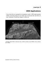
DEM Applications

Can a laser device mounted in an airplane create a GIS-ready ground
surface elevation map of your study area or measure the elevation of
your manholes? Read this chapter to find out.

1:250,000 USGS DEM for Mariposa East, California (plotted using DEM3D viewer software
from USGS).

2097_C004.fm Page 75 Monday, December 6, 2004 6:00 PM
Copyright © 2005 by Taylor & Francis



LEARNING OBJECTIVE

The learning objective of this chapter is to learn how to use digital elevation models
(DEM) in GIS for water industry applications.

MAJOR TOPICS

• DEM basics
• DEM data resolution and accuracy
• USGS DEM data
• DEM data from remote sensing technology

• DEM data from LIDAR and IFSAR technologies
• DEM analysis techniques and software packages
• DEM application case studies and examples

LIST OF CHAPTER ACRONYMS

3-D

Three-Dimensional

DEM

Digital Elevation Model

DTM

Digital Terrain Model

ERDAS

Earth Resource Data Analysis System

IFSAR

Interferometric Synthetic Aperture Radar

LIDAR

Laser Imaging Detection and Ranging/Light Imaging Detection and Ranging

NED

National Elevation Detection and Ranging

TIN

Triangular Irregular Network

HYDROLOGIC MODELING OF THE BUFFALO BAYOU
USING GIS AND DEM DATA

In the 1970s, the Hydrologic Engineering Center (HEC) of the U.S. Army Corps
of Engineers participated in developing some of the earliest GIS applications to meet
the H&H modeling needs in water resources. In the 1990s, HEC became aware of
the phenomenal growth and advancement in GIS. The capability of obtaining spatial
data from the Internet coupled with powerful algorithms in software and hardware
made GIS an attractive tool for water resources projects. The Buffalo Bayou Water-
shed covers most of the Houston metropolitan area in Texas. The first recorded flood
in 1929 in the watershed devastated the city of Houston. Since then, other flooding
events of similar vigor and intensity have occurred. During 1998 to 1999, the
hydrologic modeling of this watershed was conducted using the Hydrologic Mod-
eling System (HMS) with inputs derived from GIS. The watersheds and streams
were delineated from the USGS DEM data at 30-m cell resolution, stream data from
USGS digital line graph (DLG), and EPA river reach file (RF1). When used sepa-
rately, software packages such as ArcInfo, ArcView, and Data Storage System (DSS)

2097_C004.fm Page 76 Monday, December 6, 2004 6:00 PM
Copyright © 2005 by Taylor & Francis

were found to be time consuming, requiring the combined efforts of many people.
HEC integrated these existing software tools with new programs developed in this
project into a comprehensive GIS software package called HEC-GeoHMS. The low-
relief terrain of the study area required human interpretation of drainage paths, urban
drainage facilities, and man-made hydraulic structures (e.g., culverts and storm
drains), which dictated flow patterns that could not be derived from DEM terrain
representation. To resolve this issue, the project team took advantage of the flexibility
in HMS to correct drainage patterns according to human interpretations and local
knowledge (Doan, 1999).

DEM BASICS

Topography influences many processes associated with the geography of the
Earth, such as temperature and precipitation. GIS application professionals must be
able to represent the Earth’s surface accurately because any inaccuracies can lead
to poor decisions that may adversely impact the Earth’s environment. A DEM is a
numerical representation of terrain elevation. It stores terrain data in a grid format
for coordinates and corresponding elevation values. DEM data files contain infor-
mation for the digital representation of elevation values in a raster form. Cell-based
raster data sets, or grids, are very suitable for representing geographic phenomena
that vary continuously over space such as elevation, slope, precipitation, etc. Grids
are also ideal for spatial modeling and analysis of data trends that can be represented
by continuous surfaces, such as rainfall and stormwater runoff.
DEM data are generally stored using one of the following three data structures:

• Grid structures
• Triangular irregular network (TIN) structures
• Contour-based structures

Regardless of the underlying data structure, most DEMs can be defined in terms
of (x,y,z) data values, where x and y represent the location coordinates and z
represents the elevation values. Grid DEMs consist of a sampled array of elevations
for a number of ground positions at regularly spaced intervals. This data structure
creates a square grid matrix with the elevation of each grid square, called a pixel,
stored in a matrix format. Figure 4.1 shows a 3D plot of grid-type DEM data. As
shown in Figure 4.2, TINs represent a surface as a set of nonoverlapping contiguous
triangular facets, of irregular size and shape. Digital terrain models (DTMs) and
digital surface models (DSMs) are different varieties of DEM. The focus of this
chapter is on grid-type DEMs.
Usually, some interpolation is required to determine the elevation value from a
DEM for a given point. The DEM-based point elevations are most accurate in
relatively flat areas with smooth slopes. DEMs produce low-accuracy point elevation
values in areas with large and abrupt changes in elevation, such as cliffs and road
cuts (Walski et al., 2001).

2097_C004.fm Page 77 Monday, December 6, 2004 6:00 PM
Copyright © 2005 by Taylor & Francis



Figure 4.1

Grid-type DEM.

Figure 4.2

TIN-type DEM.

2097_C004.fm Page 78 Monday, December 6, 2004 6:00 PM

Copyright © 2005 by Taylor & Francis



DEM APPLICATIONS

Major DEM applications include (USGS, 2000):

• Delineating watershed boundaries and streams
• Developing parameters for hydrologic models
• Modeling terrain gravity data for use in locating energy resources
• Determining the volume of proposed reservoirs
• Calculating the amount of material removed during strip mining
• Determining landslide probability

Jenson and Dominique (1988) demonstrated that drainage characteristics could
be defined from a DEM. DEMs can be used for automatic delineation of watershed
and sewershed boundaries. DEM data can be processed to calculate various water-
shed and sewershed characteristics that are used for H&H modeling of watersheds
and sewersheds. DEMs can create shaded relief maps that can be used as base maps
in a GIS for overlaying vector layers such as water and sewer lines. DEM files may
be used in the generation of graphics such as isometric projections displaying slope,
direction of slope (aspect), and terrain profiles between designated points. This aspect
identifies the steepest downslope direction from each cell to its neighbors.
Raster GIS software packages can convert the DEMs into image maps for visual
display as layers in a GIS. DEMs can be used as source data for digital orthophotos.
They can be used to create digital orthophotos by orthorectification of aerial photos,
as described in Chapter 3 (Remote Sensing Applications). DEMs can also serve as
tools for many activities including volumetric analysis and site location of towers.
DEM data may also be combined with other data types such as stream locations and

weather data to assist in forest fire control, or they may be combined with remote
sensing data to aid in the classification of vegetation.

Three-Dimensional (3D) Visualization

Over the past decade, 3D computer modeling has evolved in most of the engi-
neering disciplines including, but not limited to, layout, design, and construction of
industrial and commercial facilities; landscaping; highway, bridge, and embankment
design; geotechnical engineering; earthquake analysis; site planning; hazardous-waste
management; and digital terrain modeling. The 3D visualization can be used for
landscape visualizing or fly-through animation movies of the project area. 3D anima-
tions are highly effective tools for public- and town-meeting presentations. GIS can
be used to create accurate topographic elevation models and generate precise 3D data.
A DEM is a powerful tool and is usually as close as most GISs get to 3D modeling.
3D graphics are commonly used as a visual communication tool to display a
3D view of an object on two-dimensional (2D) media (e.g., a paper map). Until
the early 1980s, a large mainframe computer was needed to view, analyze, and
print objects in 3D graphics format. Hardware and software are now available for
3D modeling of terrain and utility networks on personal computers. Although DEMs
are raster images, they can be imported into 3D visualizations packages. Affordable
and user-friendly software tools are bringing more users into the world of GIS.

2097_C004.fm Page 79 Monday, December 6, 2004 6:00 PM
Copyright © 2005 by Taylor & Francis



These software tools and 3D data can be used to create accurate virtual reality
representations of landscape and infrastructure with the help of stereo imagery and
automatic extraction of 3D information. For example, Skyline Software System’s

(www.skylinesoft.com) TerraExplorer provides realistic, interactive, photo-based
3D maps of many locations and cities of the world on the Internet.
Satellite imagery is also driving new 3D GIS applications. GIS can be used to
precisely identify a geographic location in 3D space and link that location and its
attributes through the integration of photogrammetry, remote sensing, GIS, and 3D
visualization. 3D geographic imaging is being used to create orthorectified imagery,
DEMs, stereo models, and 3D features.

DEM RESOLUTION AND ACCURACY

The accuracy of a DEM is dependent upon its source and the spatial resolution
(grid spacing). DEMs are classified by the method with which they were prepared
and the corresponding accuracy standard. Accuracy is measured as the root mean
square error (RMSE) of linearly interpolated elevations from the DEM, compared
with known elevations. According to RMSE classification, there are three levels of
DEM accuracy (Walski et al., 2001):

• Level 1: Based on high-altitude photography, these DEMs have the lowest accu-
racy. The vertical RMSE is 7 m and the maximum permitted RMSE is 15 m.
• Level 2: These are based on hypsographic and hydrographic digitization, followed
by editing to remove obvious errors. These DEMs have medium accuracy. The
maximum permitted RMSE is one half of the contour interval.
• Level 3: These are based on USGS digital line graph (DLGs) data (Shamsi, 2002).
The maximum permitted RMSE is one third of the contour interval.

The vertical accuracy of 7.5-min DEMs is greater than or equal to 15 m. Thus,
the 7.5-min DEMs are suitable for projects at 1:24,000 scale or smaller (Zimmer,
2001a). A minimum of 28 test points per DEM are required (20 interior points and
8 edge points). The accuracy of the 7.5-min DEM data, together with the data
spacing, adequately support computer applications that analyze hypsographic fea-

tures to a level of detail similar to manual interpretations of information as printed
at map scales not larger than 1:24,000. Early DEMs derived from USGS quadrangles
suffered from mismatches at boundaries (Lanfear, 2000).
DEM selection for a particular application is generally driven by data availability,
judgment, experience, and test applications (ASCE, 1999). For example, because
no firm guidelines are available for selection of DEM characteristics for hydrologic
modeling, a hydrologic model might need 30-m resolution DEM data but might
have to be run with 100-m data if that is the best available data for the study area.
In the U.S., regional-scale models have been developed at scales of 1:250,000 to
1:2,000,000 (Laurent et al., 1998). Seybert (1996) concluded that modeled watershed
runoff peak flow values are more sensitive to changes in spatial resolution than
modeled runoff volumes. An overall subbasin area to grid–cell area ratio of 10

2

was
found to produce reasonable model results.

2097_C004.fm Page 80 Monday, December 6, 2004 6:00 PM
Copyright © 2005 by Taylor & Francis



The grid size and time resolution used for developing distributed hydrologic
models for large watersheds is a compromise between the required accuracy, available
data accuracy, and computer run-time. Finer grid size requires more computing time,
more extensive data, and more detailed boundary conditions. Chang et al. (2000)
conducted numerical experiments to determine an adequate grid size for modeling
large watersheds in Taiwan where 40 m

×

40 m resolution DEM data are available.
They investigated the effect of grid size on the relative error of peak discharge and
computing time. Simulated outlet hydrographs showed higher peak discharge as the
computational grid size was increased. In a study, for a watershed of 526 km

2

located
in Taiwan, a grid resolution of 200 m

×

200 m was determined to be adequate.
Table 4.1 shows suggested DEM resolutions for various applications (Maidment,
1998). Large (30-m) DEMs are recommended for water distribution modeling (Wal-
ski et al., 2001).
The size of a DEM file depends on the DEM resolution, i.e., the finer the DEM
resolution, the smaller the grid, and the larger the DEM file. For example, if the
grid size is reduced by one third, the file size will increase nine times. Plotting and
analysis of high-resolution DEM files are slower because of their large file sizes.

USGS DEMS

In the U.S., the USGS provides DEM data for the entire country as part of the
National Mapping Program. The National Mapping Division of USGS has scanned
all its paper maps into digital files, and all 1:24,000-scale quadrangle maps now
have DEMs (Limp, 2001).
USGS DEMs are the (x,y,z) triplets of terrain elevations at the grid nodes of the

Universal Transverse Mercator (UTM) coordinate system referenced to the North
American Datum of 1927 (NAD27) or 1983 (NAD83) (Shamsi, 1991). USGS DEMs
provide distance in meters, and elevation values are given in meters or feet relative
to the National Geodetic Vertical Datum (NGVD) of 1929. The USGS DEMs are
available in 7.5-min, 15-min, 2-arc-sec (also known as 30-min), and 1˚ units. The
7.5- and 15-min DEMs are included in the large-scale category, whereas 2-arc-sec
DEMs fall within the intermediate-scale category and 1˚ DEMs fall within the small-
scale category. Table 4.2 summarizes the USGS DEM data types.
This chapter is mostly based on applications of 7.5-min USGS DEMs. The
DEM data for 7.5-min units correspond to the USGS 1:24,000-scale topographic
quadrangle map series for all of the U.S. and its territories. Thus, each 7.5-min

Table 4.1

DEM Applications
DEM
Resolution
Approximate
Cell Size
Watershed
Area (km

2

)
Typical
Application

1 sec 30 m 5 Urban watersheds
3 sec 100 m 40 Rural watersheds

15 sec 500 m 1,000 River basins, States
30 sec 1 km 4,000 Nations
3 min 5 km 150,000 Continents
5 min 10 km 400,000 World

2097_C004.fm Page 81 Monday, December 6, 2004 6:00 PM
Copyright © 2005 by Taylor & Francis



by 7.5-min block provides the same coverage as the standard USGS 7.5-min map
series. Each 7.5-min DEM is based on 30-m by 30-m data spacing; therefore, the
raster grid for the 7.5-min USGS quads are 30 m by 30 m. That is, each 900 m

2

of land surface is represented by a single elevation value. USGS is now moving
toward acquisition of 10-m accuracy (Murphy, 2000).

USGS DEM Formats

USGS DEMs are available in two formats:

1. DEM file format: This older file format stores DEM data as ASCII text, as shown
in Figure 4.3. These files have a file extension of dem (e.g., lewisburg_PA.dem).
These files have three types of records (Walski et al., 2001):
• Type A: This record contains information about the DEM, including name,
boundaries, and units of measurements.

Table 4.2

USGS DEM Data Formats
DEM Type Scale Block Size Grid Spacing

Large 1:24,000 7.5 ft

×

7.5 ft 30 m
Intermediate Between large and small 30 ft

×

30 ft 2 sec
Small 1:250,000 1

°



×

1

°

3 sec

Figure 4.3

USGS DEM file.

2097_C004.fm Page 82 Monday, December 6, 2004 6:00 PM
Copyright © 2005 by Taylor & Francis



• Type B: These records contain elevation data arranged in “profiles” from south
to north, with the profiles organized from west to east. There is one Type-B
record for each south–north profile.
• Type C: This record contains statistical information on the accuracy of DEM.
2. Spatial Data Transfer Standard (SDTS): This is the latest DEM file format that
has compressed data for faster downloads. SDTS is a robust way of transferring
georeferenced spatial data between dissimilar computer systems and has the poten-
tial for transfer with no information loss. It is a transfer standard that embraces
the philosophy of self-contained transfers, i.e., spatial data, attribute, georeferenc-
ing, data quality report, data dictionary, and other supporting metadata; all are
included in the transfer. SDTS DEM data are available as tar.gz compressed files.
Each compressed file contains 18 ddf files and two readme text files. For further
analysis, the compressed SDTS files should be unzipped (uncompressed). Stan-
dard zip programs, such as PKZIP, can be used for this purpose.

Some DEM analysis software may not read the new SDTS data. For such
programs, the user should translate the SDTS data to a DEM file format. SDTS
translator utilities, like SDTS2DEM or MicroDEM, are available from the GeoCom-
munity’s SDTS Web site to convert the SDTS data to other file formats.

National Elevation Dataset (NED)

Early DEMs were derived from USGS quadrangles, and mismatches at bound-

aries continued to plague the use of derived drainage networks for larger areas
(Lanfear, 2000). The NED produced by USGS in 1999 is the new generation of
seamless DEM that largely eliminates problems of quadrangle boundaries and other
artifacts. Users can now select DEM data for their area of interest.
The NED has been developed by merging the highest resolution, best-quality
elevation data available across the U.S. into a seamless raster format. NED is designed
to provide the U.S. with elevation data in a seamless form, with a consistent datum,
elevation unit, and projection. Data corrections were made in the NED assembly
process to minimize artifacts, perform edge matching, and fill sliver areas of missing
data. NED is the result of the maturation of the USGS effort to provide 1:24,000-
scale DEM data for the conterminous U.S. and 1:63,360-scale DEM data for Alaska.
NED has a resolution of 1 arc-sec (approximately 30 m) for the conterminous U.S.,
Hawaii, and Puerto Rico and a resolution of 2 arc-sec for Alaska. Using a hill-shade
technique, USGS has also derived a shaded relief coverage that can be used as a base
map for vector themes. Other themes, such as land use or land cover, can be draped
on the NED-shaded relief maps to enhance the topographic display of themes. The
NED store offers seamless data for sale, by user-defined area, in a variety of formats.

DEM DATA AVAILABILITY

USGS DEMs can be downloaded for free from the USGS geographic data
download Web site. DEM data on CD-ROM can also be purchased from the USGS
EarthExplorer Web site for an entire county or state for a small fee to cover the
shipping and handling cost. DEM data for other parts of the world are also available.

2097_C004.fm Page 83 Monday, December 6, 2004 6:00 PM
Copyright © 2005 by Taylor & Francis

The 30 arc-sec DEMs (approximately 1 km

2

square cells) for the entire world have
been developed by the USGS Earth Resources Observation Systems (EROS) Data
Center and can be downloaded from the USGS Web site. More information can be
found on the Web site of the USGS node of the National Geospatial Data Clearing-
house. State or regional mapping and spatial data clearinghouse Web sites are the
most valuable source of free local spatial data. For example, the Pennsylvania Spatial
Data Access system (PASDA), Pennsylvania's official geospatial information clear-
inghouse and its node on the National Spatial Data Infrastructure (NSDI), provides
free downloads of DEM and other spatial data.

DEM DATA CREATION FROM REMOTE SENSING

In February 2000, NASA flew one of its most ambitious missions, using the
space shuttle

Endeavor

to map the entire Earth from 60˚ north to 55˚ south of the
equator. Mapping at a speed of 1747 km

2

every second, the equivalent of mapping
the state of Florida in 97.5 sec, the Shuttle Radar Topography Mission (SRTM)
provided 3D data of more than 80% of Earth’s surface in about 10 days. The SRTM
data will provide a 30-m DEM coverage for the entire world (Chien, 2000).

Topographic elevation information can be automatically extracted from remote sens-
ing imagery to create highly accurate DEMs. There are two ways in which DEM data
can be created using remote sensing methods: image processing and data collection.

Image Processing Method

The first method uses artificial intelligence techniques to automatically extract
elevation information from the existing imagery. Digital image-matching methods
commonly used for machine vision automatically identify and match image point
locations of a ground point appearing on overlapping areas of a stereo pair (i.e., left-
and right-overlapping images). Once the correct image positions are identified and
matched, the ground point elevation is computed automatically. For example, the
French satellite SPOT’s stereographic capability can generate topographic data. USGS
Earth Observing System’s (EOS) Terra satellite can provide DEMs from stereo images.
Off-the-shelf image processing software products are available for automatic
extraction of DEM data from remote sensing imagery. For instance, Leica Geosys-
tems’ IMAGINE OrthoBASE Pro software can be used to automatically extract
DEMs from aerial photography, satellite imagery (IKONOS, SPOT, IRS-1C), and
digital video and 35-mm camera imagery. It can also subset and mosaic 500 or more
individual DEMs. The extracted DEM data can be saved as raster DEMs, TINs,
ESRI 3D Shapefiles, or ASCII output (ERDAS, 2001b).

Data Collection Method

In this method, actual elevation data are collected directly using lasers. This
method uses laser-based LIDAR and radar-based IFSAR systems described in the
following text.

2097_C004.fm Page 84 Monday, December 6, 2004 6:00 PM
Copyright © 2005 by Taylor & Francis

LIDAR

Unlike photogrammetric techniques, which can be time consuming and expensive
for large areas, this method is a cost-effective alternative to conventional technologies.
It can create DEMs with accuracy levels ranging from 20 to 100 cm, which are
suitable for many engineering applications. This remote-sensing technology does not
even involve an image. Laser imaging detection and ranging (LIDAR) is a new system
for measuring ground surface elevation from an airplane. LIDAR can collect 3D
digital data on the fly. LIDAR sensors provide some of the most accurate elevation
data in the shortest time ever by bouncing laser beams off the ground. LIDAR
technology, developed in the mid-1990s, combines global positioning system (GPS),
precision aircraft guidance, laser range finding, and high-speed computer processing
to collect ground elevation data. Mounted on an aircraft, a high-accuracy scanner
sweeps the laser pulses across the flight path and collects reflected light. A laser
range-finder measures the time between sending and receiving each laser pulse to
determine the ground elevation below. The LIDAR system can survey up to 10,000
acres per day and provide horizontal and vertical accuracies up to 12 and 6 in.,
respectively. Chatham County, home of Savannah, Georgia, used the LIDAR approach
to collect 1-ft interval contour data for the entire 250,000 acre county in less than a
year. The cost of conventional topographic survey for this data would be over $20
million. The County saved $7 million in construction cost by using data from Airborne
Laser Terrain Mapping (ALTM) technology, a LIDAR system manufactured by
Optech, Canada. The new ALTM data were used to develop an accurate hydraulic
model of the Hardin basin (Stones, 1999).

Chatham County, Georgia, saved $7 million in construction cost by using LIDAR data.

Boise-based Idaho Power Company spent $273,000 on LIDAR data for a 290
km stretch of the rugged Hell’s Canyon, through which the Snake River runs. The
cost of LIDAR data was found to be less than aerial data and expensive ground-
surveying. The company used LIDAR data to define the channel geometry, combined
it with bathymetry data, and created digital terrain files containing ten cross sections
of the canyon per mile. The cross-section data were input to a hydraulic model that
determined the effect of power plants’ releases on vegetation and wildlife habitats
(Miotto, 2000).

IFSAR

Interferometric Synthetic Aperture Radar (IFSAR) is an aircraft-mounted radar
system for quick and accurate mapping of large areas in most weather conditions
without ground control. Because it is an airborne radar, IFSAR collects elevation
data on the first try in any weather (regardless of fog, clouds, or rain), day or night,
significantly below the cost of satellite-derived DEM. The IFSAR process measures
elevation data at a much denser grid than photogrammetric techniques, using over-
lapping stereo images. A denser DEM provides a more detailed terrain surface in

2097_C004.fm Page 85 Monday, December 6, 2004 6:00 PM
Copyright © 2005 by Taylor & Francis



an image. IFSAR is efficient because it derives the DEM data by digital processing
of a single radar image. This allows elevation product delivery within days of data
collection. A DEM with a minimum vertical accuracy of 2 m is necessary to achieve
the precision level orthorectification for IKONOS imagery. DEMs generated from
the IFSAR data have been found to have the adequate vertical accuracy to orthorec-
tify IKONOS imagery to the precision level (Corbley, 2001).

Intermap Technologies’ (Englewood, Colorado, www.intermaptechnologies.
com) Lear jet-mounted STAR-3i system, an airborne mapping system, has been
reported to provide simultaneous high-accuracy DEMs and high-resolution orthorec-
tified imagery without ground control. STAR-3i IFSAR system typically acquires
elevation points at 5-m intervals, whereas photogrammetric sources use a spacing of
30 to 50 m. STAR-3i can provide DEMs with a vertical accuracy of 30 cm to 3 m
and an orthoimage resolution of 2.5 m.

DEM ANALYSIS
Cell Threshold for Defining Streams

Before starting DEM analysis, users must define the minimum number of
upstream cells contributing flow into a cell to classify that cell as the origin of a
stream. This number, referred to as the cell “threshold,” defines the minimum
upstream drainage area necessary to start and maintain a stream. For example, if a
stream definition value of ten cells is specified, then for a single grid location of the
DEM to be in a stream, it must drain at least ten cells. It is assumed that there is
flow in a stream if its upstream area exceeds the critical threshold value. In this case,
the cell is considered to be a part of the stream. The threshold value can be estimated
from existing topographic maps or from the hydrographic layer of the real stream
network. Selection of an appropriate cell threshold size requires some user judgment.
Users may start the analysis with an assumed or estimated value and adjust the initial
value by comparing the delineation results with existing topographic maps or hydro-
graphic layers. The cell threshold value directly affects the number of subbasins
(subwatersheds or subareas). A smaller threshold results in smaller subbasin size,
larger number of subbasins, and slower computation speed for the DEM analysis.

The D-8 Model

The 8-direction pour point model, also known as the D-8 model, is a commonly

used algorithm for delineating a stream network from DEMs. As shown in Figure 4.4,
it identifies the steepest downslope flow path between each cell and its eight neigh-
boring cells. This path is the only flow path leaving the cell. Watershed area is
accumulated downslope along the flow paths connecting adjacent cells. The drainage
network is identified from the user-specified threshold area at the bottom of which
a source channel originates and classifies all cells with a greater watershed area as
part of the drainage network. Figure 4.4 shows stream delineation steps using the
D-8 model with a cell threshold value of ten cells. Grid A shows the cell elevation

2097_C004.fm Page 86 Monday, December 6, 2004 6:00 PM
Copyright © 2005 by Taylor & Francis



values. Grid B shows flow direction arrows based on calculated cell slopes. Grid C
shows the number of accumulated upstream cells draining to each cell. Grid D shows
the delineated stream segment based on the cells with flow accumulation values
greater than or equal to ten.

DEM Sinks

The D-8 and many other models do not work well in the presence of depressions,
sinks, and flat areas. Some sinks are caused by the actual conditions, such as the
Great Salt Lake in Utah where no watershed precipitation travels through a river
network toward the ocean. The sinks are most often caused by data noise and errors
in elevation data. The computation problems arise because cells in depressions, sinks,
and flat areas do not have any neighboring cells at a lower elevation. Under these
conditions, the flow might accumulate in a cell and the resulting flow network may
not necessarily extend to the edge of the grid. Unwanted sinks must be removed
prior to starting the stream or watershed delineation process by raising the elevation

of the cells within the sink to the elevation of its lowest outlet. Most raster GIS
software programs provide a FILL function for this purpose. For example, ArcInfo’s
GRID extension provides a FILL function that raises the elevation of the sink cells
until the water is able to flow out of it.
The FILL approach assumes that all sinks are caused by underestimated elevation
values. However, the sinks can also be created by overestimated elevation values,
in which case breaching of the obstruction is more appropriate than filling the sink
created by the obstruction. Obstruction breaching is particularly effective in flat or
low-relief areas (ASCE, 1999).

Figure 4.4

Figure 11-4. D-8 Model for DEM-based stream delineation (A) DEM elevation grid,
(B) flow direction grid, (C) flow accumulation grid, and (D) delineated streams for
cell threshold of ten.

2097_C004.fm Page 87 Monday, December 6, 2004 6:00 PM
Copyright © 2005 by Taylor & Francis



Stream Burning

DEM-based stream or watershed delineations may not be accurate in flat areas
or if the DEM resolution failed to capture important topographic information. This
problem can be solved by “burning in” the streams using known stream locations
from the existing stream layers. This process modifies the DEM grid so that the flow
of water is forced into the known stream locations. The cell elevations are artificially
lowered along the known stream locations or the entire DEM is raised except along
known stream paths. The phrase

burning in

indicates that the streams have been
forced, or “burned” into the DEM topography (Maidment, 2000). This method must
be used with caution because it may produce flow paths that are not consistent with
the digital topography (ASCE, 1999).

DEM Aggregation

Distributed hydrologic models based on high-resolution DEMs may require
extensive computational and memory resources that may not be available. In this
case, high-resolution DEMs can be aggregated into low-resolution DEMs. For exam-
ple, it was found that the 30-m USGS DEM would create 80,000 cells for the
72.6 km

2

Goodwater Creek watershed located in central Missouri. Distributed mod-
eling of 80,000 cells was considered time consuming and impractical (Wang et al.,
2000). The 30 m

×

30 m cells were, therefore, aggregated into 150 m x 150 m
(2.25 ha) cells. In other words, 25 smaller cells were aggregated into one large cell,
which reduced the number of cells from 80,000 to approximately 3,000. Best of all,
the aggregated DEM produced the same drainage network as the original DEM. The
aggregation method computes the flow directions of the coarse-resolution cells based
on the flow paths defined by the fine-resolution cells. It uses three steps: (1) determine

the flow direction of the fine-resolution DEM, (2) determine outlets of coarse-
resolution DEM, and (3) approximate the flow direction of coarse-resolution DEM,
based on the flow direction of the fine-resolution DEM.

Slope Calculations

Subbasin slope is an input parameter in many hydrologic models. Most raster
GIS packages provide a SLOPE function for estimating slope from a DEM. For
example, ERDAS IMAGINE software uses its SLOPE function to compute percent
slope by fitting a plane to a pixel elevation and its eight neighboring pixel elevations.
The difference in elevation between the low and the high points is divided by the
horizontal distance and multiplied by 100 to compute percent slope for the pixel.
Pixel slope values are averaged to compute the mean percent slope of each subbasin.

SOFTWARE TOOLS

The DEM analysis functions described in the preceding subsections require
appropriate software. Representative DEM analysis software tools and utilities are
listed in Table 4.3.

2097_C004.fm Page 88 Monday, December 6, 2004 6:00 PM
Copyright © 2005 by Taylor & Francis



Table 4.3

Sample DEM Analysis Software Tools
Software Vendor and Web site Notes

Spatial Analyst
and Hydro extension
ESRI, Redlands, California
www.esri.com
ArcGIS 8.x and ArcView
3.x extension
ARC GRID extension ArcInfo 7.x extension
Analyst ArcGIS 8.x



and ArcView 3.x



extension
IDRISI Clark University Worcester, Massachusetts
www.clarklabs.org
ERDAS IMAGINE Leica Geosystems, Atlanta, Georgia
gis.leica-geosystems.com
www.erdas.com
Formerly, Earth Resource
Data Analysis System
(ERDAS) software
TOPAZ U.S. Department of Agriculture,
Agricultural Research Service, El Reno, Oklahoma
grl.ars.usda.gov/topaz/TOPAZ1.HTM
MicroDEM U.S. Naval Academy
www.usna.edu/Users/oceano/pguth/website/microdem.htm
Software developed by

Peter Guth of the
Oceanography Department
DEM3D viewer USGS, Western Mapping Center, Menlo Park, California
craterlake.wr.usgs.gov/dem3d.html
Free download, allows
viewing of DEM files through
a 3D perspective

2097_C004.fm Page 89 Monday, December 6, 2004 6:00 PM
Copyright © 2005 by Taylor & Francis



Some programs such as Spatial Analyst provide both the DEM analysis and
hydrologic modeling capabilities. ASCE (1999) has compiled a review of hydrologic
modeling systems that use DEMs. Major DEM software programs are discussed in
the following text.

Spatial Analyst and Hydro Extension

Spatial Analyst is an optional extension (separately purchased add-on program)
for ESRI’s ArcView 3.x and ArcGIS 8.x software packages. The Spatial Analyst
Extension adds raster GIS capability to the ArcView and ArcGIS vector GIS soft-
ware. Spatial Analyst allows for use of raster and vector data in an integrated
environment and enables desktop GIS users to create, query, and analyze cell-based
raster maps; derive new information from existing data; query information across
multiple data layers; and integrate cell-based raster data with the traditional vector
data sources. It can be used for slope and aspect mapping and for several other
hydrologic analyses, such as delineating watershed boundaries, modeling stream
flow, and investigating accumulation. Spatial Analyst for ArcView 3.x has most, but

not all, of the functionality of the ARC GRID extension for ArcInfo 7.x software
package described below.
Spatial Analyst for ArcView 3.x is supplied with a Hydro (or hydrology) exten-
sion that further extends the Spatial Analyst user interface for creating input data
for hydrologic models. This extension provides functionality to create watersheds
and stream networks from a DEM, calculate physical and geometric properties of
the watersheds, and aggregate these properties into a single-attribute table that can
be attached to a grid or Shapefile. Hydro extension requires that Spatial Analyst be
already installed. Hydro automatically loads the Spatial Analyst if it is not loaded.
Depending upon the user needs, there are two approaches to using the Hydro
extension:

1. Hydro pull-down menu options: If users only want to create watershed subbasins
or the stream network, they should work directly with the Hydro pull-down
menu options (Figure 4.5). Table 4.4 provides a brief description of each of
these menu options. “Fill Sinks” works off an active elevation grid theme. “Flow
Direction” works off an active elevation grid theme that has been filled. “Flow
Accumulation” works off an active flow direction grid theme. “Flow Length”
works off an active flow direction grid theme. “Watershed” works off an active
flow accumulation grid theme and finds all basins in the data set based on a
minimum number of cells in each basin. The following steps should be performed
to create watersheds using the Hydro pull-down menu options, with the output
grid from each step serving as the input grid for the next step:
• Import the raw USGS DEM.
• Fill the sinks using the “Fill Sinks” menu option (input = raw USGS DEM).
This is a very important intermediate step. Though some sinks are valid, most
are data errors and should be filled.
• Compute flow directions using the “Flow Direction” menu option (input =
filled DEM grid).
• Compute flow accumulation using the “Flow Accumulation” menu option

(input = flow directions grid).

2097_C004.fm Page 90 Monday, December 6, 2004 6:00 PM
Copyright © 2005 by Taylor & Francis



• Delineate streams using the “Stream Network” menu option (input = flow
accumulation grid).
• Delineate watersheds using the “Watershed” menu option.
2. Hydrologic Modeling Dialogue: If users want to create subbasins and calculate many
additional attributes for them, they should use the Hydrologic Modeling Dialogue
(Figure 4.6), which is the first choice under the Hydro pull-down menu. The Hydro-
logic Modeling Dialogue is designed to be a quick one-step method for calculating
and then aggregating a set of watershed attributes to a single file. This file can then
be used in a hydrologic model, such as the Watershed Modeling System (WMS)
(discussed in Chapter 11 [Modeling Applications]), or it can be reformatted for input
into HEC’s HMS model, or others. The following steps should be performed to
create watersheds using the Hydrologic Modeling Dialogue:
• Choose “Delineate” from DEM and select an elevation surface.
• Fill the sinks when prompted.
• Specify the cell threshold value when prompted. This will create watersheds
based on the number of cells or up-slope area defined by the user as the smallest
watershed wanted.

Additional DEM analysis resources (tutorials, exercises, sample data, software
utilities, reports, papers, etc.) are provided at the following Web sites:

• ESRI Web site at www.esri.com/arcuser/ (do a search for “Terrain Modeling”)
• University of Texas at Austin (Center for Research in Water Resources) Web site

at www.crwr.utexas.edu/archive.shtml

The last four Hydro options (Table 4.4) work with existing data layers. They do
not create elevation, slope, precipitation, and runoff curve number layers. They

Figure 4.5

Hydro extension pull-down menu.

2097_C004.fm Page 91 Monday, December 6, 2004 6:00 PM
Copyright © 2005 by Taylor & Francis



simply compute mean areal values of these four parameters for the subbasins, using
the existing GIS layers of these parameters. Thus, the GIS layers of elevation, slope,
precipitation, and runoff curve number must be available to use the mean functions
of the Hydro extension.
Figure 4.7 shows Hydro’s raindrop or pour point feature. Using this capability,
the user can trace the flow path from a specified point to the watershed outlet. Hydro
also calculates a flow length as the maximum distance along the flow path within
each watershed. The flow path can be divided by the measured or estimated velocity
to estimate the time of concentration or travel time that are used to estimate runoff
hydrographs. Travel time can also be used to estimate the time taken by a hazardous
waste spill to reach a sensitive area or water body of the watershed. Laurent et al.
(1998) used this approach to estimate travel time between any point of a watershed
and a water resource (river or well). This information was further used to create a
map of water resources vulnerability to dissolved pollution in an area in Massif
Central, France. Subbasin area can be divided by flow length to estimate the overland
flow width for input to a rainfall-runoff model such as EPA’s Storm Water Manage-

ment Model (SWMM).

Table 4.4

Hydro Extension Menu Options
Hydro Menu Option Function

Hydrologic modeling Creates watersheds and calculates their attributes
Flow direction Computes the direction of flow for each cell in a DEM
Identify sinks Creates a grid showing the location of sinks or areas of
internal drainage in a DEM
Fill sinks Fills the sinks in a DEM, creating a new DEM
Flow accumulation Calculates the accumulated flow or number of up-slope
cells, based on a flow direction grid
Watershed Creates watersheds based upon a user-specified flow
accumulation threshold
Area Calculates the area of each watershed in a watershed
grid
Perimeter Calculates the perimeter of each watershed in a
watershed grid
Length Calculates the straight-line distance from the pour
point to the furthest perimeter point for each watershed
Flow length Calculates the length of flow path for each cell
to the pour point for each watershed
Flow length by watershed Calculates the maximum distance along the flow path
within each watershed
Shape factor by watershed Calculates a shape factor (watershed length squared
and then divided by watershed area) for each watershed
Stream network as line shape Creates a vector stream network from a flow
accumulation grid, based on a user-specified threshold

Centroid as point shape Creates a point shape file of watershed centroids
Pour points as point shape Creates a point shape file of watershed pour points
Mean elevation Calculates the mean elevation within each watershed
Mean slope Calculates the mean slope within each watershed
Mean precipitation Calculates the mean precipitation in each watershed
Mean curve number Calculates the mean curve number for each watershed

2097_C004.fm Page 92 Monday, December 6, 2004 6:00 PM
Copyright © 2005 by Taylor & Francis



ARC GRID Extension

ARC GRID is an optional extension for ESRI’s ArcInfo



7.x GIS software
package. GRID adds raster geoprocessing and hydrologic modeling capability to the
vector-based ArcInfo GIS. For hydrologic modeling, the extension offers a Hydro-
logic Tool System and several hydrologically relevant functions for watershed and
stream network delineation.
The FLOWDIRECTION function creates a grid of flow directions from each
cell to the steepest downslope neighbor. The results of FLOWDIRECTION are used
in many subsequent functions such as stream delineation. The FLOWACCUMULA-
TION function calculates upstream area or cell-weighted flow draining into each
cell. The WATERSHED function delineates upstream tributary area at any user-
specified point, channel junction, or basin outlet cell. This function requires step-
by-step calculations. Arc Macro Language (AML) programs can be written to auto-

mate this function for delineating subbasins at all the stream nodes.
GRID can find upstream or downstream flow paths from any cell and determine
their lengths. GRID can perform stream ordering and assign unique identifiers to
the links of a stream network delineated by GRID. Spatial intersection between
streams and subbasins can define the links between the subbasins and streams. This
method relates areal attributes such as subbasin nutrient load to linear objects such
as streams. The NETWORK function can then compute the upstream accumulated
nutrient load for each stream reach (Payraudeau et al., 2000). This approach is also
useful in DEM-based runoff quality modeling.

Figure 4.6

Hydro extension Hydrologic Modeling Dialogue.

2097_C004.fm Page 93 Monday, December 6, 2004 6:00 PM
Copyright © 2005 by Taylor & Francis



IDRISI

IDRISI is not an acronym; it is named after a cartographer born in 1099 A.D.
in Morocco, North Africa. IDRISI was developed by the Graduate School of Geog-
raphy at Clark University. IDRISI provides GIS and remote sensing software func-
tions, from database query through spatial modeling to image enhancement and
classification. Special facilities are included for environmental monitoring and nat-
ural resource management, including change and time-series analysis, multicriteria
and multiobjective decision support, uncertainty analysis (including Bayesian and
Fuzzy Set analysis), and simulation modeling (including force modeling and aniso-
tropic friction analysis). TIN interpolation, Kriging, and conditional simulation are

also offered.
IDRISI is basically a raster GIS. IDRISI includes tools for manipulating DEM
data to extract streams and watershed boundaries. IDRISI GIS data has an open
format and can be manipulated by external computer programs written by users.
This capability makes IDRISI a suitable tool for developing hydrologic modeling
applications. For example, Quimpo and Al-Medeij (1998) developed a FORTRAN

Figure 4.7

Hydro extension’s pour point feature.

2097_C004.fm Page 94 Monday, December 6, 2004 6:00 PM
Copyright © 2005 by Taylor & Francis



program to model surface runoff using IDRISI. Their approach consisted of delin-
eating watershed subbasins from DEM data and estimating subbasin runoff curve
numbers from soils and land-use data.
Figure 4.8 shows IDRISI’s DEM analysis capabilities. The upper-left window
shows a TIN model created from digital contour data. The upper-right window shows
a DEM created from the TIN with original contours overlayed. The lower-right
window shows an illuminated DEM emphasizing relief. The lower-left window
shows a false color composite image (Landsat TM bands 2, 3, and 4) draped over
the DEM (IDRISI, 2000).

TOPAZ

TOPAZ is a software system for automated analysis of landscape topography
from DEMs (Topaz, 2000). The primary objective of TOPAZ is the systematic

identification and quantification of topographic features in support of investigations
related to land-surface processes, H&H modeling, assessment of land resources,
and management of watersheds and ecosystems. Typical examples of topographic
features that are evaluated by TOPAZ include terrain slope and aspect, drainage
patterns and divides, channel network, watershed segmentation, subcatchment
identification, geometric and topologic properties of channel links, drainage dis-
tances, representative subcatchment properties, and channel network analysis
(Garbrecht and Martz, 2000). The FILL Function of TOPAZ recognizes depressions
created by embankments and provides outlets for these without filling, a better
approach than the fill-only approach in other programs (e.g., IDRISI or Spatial
Analyst).

CASE STUDIES AND EXAMPLES

Representative applications of using DEM data in GIS are described in this
section.

Watershed Delineation

A concern with streams extracted from DEMs is the precise location of streams.
Comparisons with actual maps or aerial photos often show discrepancies, especially
in low-relief landscapes (ASCE, 1999). A drainage network obtained from a DEM
must be comparable to the actual hydrologic network. Thus, it is worthwhile to
check the accuracy of DEM-based delineations. This can be done by comparing the
DEM delineations with manual delineations. Jenson (1991) found approximately
97% similarity between automatic and manual delineations from 1:50,000-scale
topographic maps.
The objective of this case study was to test the efficacy of DEM-based automatic
delineation of watershed subbasins and streams. It was assumed that manual delin-
eations are more accurate than DEM delineations. Thus, a comparison of manual

and DEM delineations was made to test the accuracy of DEM delineations.

2097_C004.fm Page 95 Monday, December 6, 2004 6:00 PM
Copyright © 2005 by Taylor & Francis



Figure 4.8

IDRISI’s DEM analysis features.

2097_C004.fm Page 96 Monday, December 6, 2004 6:00 PM
Copyright © 2005 by Taylor & Francis



The case study watershed is the Bull Run Watershed located in Union County
in north-central Pennsylvania (Shamsi, 1996). This watershed was selected because
of its small size so that readable report-size GIS maps can be printed. The proposed
technique has also been successfully applied to large watersheds with areas of several
hundred square miles. Bull Run Watershed’s 8.4 mi

2

(21.8 km

2

) drainage area is
tributary to the West Branch Susquehanna River at the eastern boundary of Lewisburg

Borough. The 7.5-min USGS topographic map of the watershed is shown in
Figure 4.9. The predominant land use in the watershed is open space and agricultural.
Only 20% of the watershed has residential, commercial, and industrial land uses.
Manual watershed subdivision was the first step of the case study. The 7.5-min
USGS topographic map of the study area was used for manual subbasin delineation,
which resulted in the 28 subbasins shown in Figure 4.9. This figure also shows the
manually delineated streams (dashed lines).
Next, ArcView Spatial Analyst and Hydro extension were used to delineate
subbasins and streams using the 7.5-min USGS DEM data. Many cell threshold values
(50, 100, 150, …, 1000) were used repeatedly to determine which DEM delineations
agreed with manual delineations. Figure 4.10, Figure 4.11, and Figure 4.12 show the
DEM subbasins for cell thresholds of 100, 250, and 500. These figures also show
the manual subbasins for comparison. It can be seen that the 100 threshold creates
too many subbasins. The 500 threshold provides the best agreement between manual
and DEM delineations.
Figure 4.13, Figure 4.14, and Figure 4.15 show the DEM streams for cell
threshold values of 100, 250, and 500. These figures also show the manually delin-
eated streams for comparison purposes. It can be seen that the 100 threshold creates
too many streams (Figure 4.13); the 500 threshold looks best (Figure 4.15) and

Figure 4.9

Bull Run Watershed showing manual subbasins and streams.

2097_C004.fm Page 97 Monday, December 6, 2004 6:00 PM
Copyright © 2005 by Taylor & Francis



provides the best agreement between the manual and DEM streams. The upper-right

boundary of the watershed in Figure 4.15 shows that one of the DEM streams crosses
the watershed boundary. This problem is referred to as the boundary “cross-over”
problem, which is not resolved by altering threshold values. It must be corrected by
manual editing of DEM subbasins or using DEM preprocessing methods such as
the stream burning method described earlier.

Figure 4.10

Manual vs. DEM subbasins for cell threshold of 100 (too many subbasins).

Figure 4.11

Manual vs. DEM subbasins for cell threshold of 250 (better).

2097_C004.fm Page 98 Monday, December 6, 2004 6:00 PM
Copyright © 2005 by Taylor & Francis



Figure 4.16 shows DEM-derived subbasin and stream maps for a portion of the
very large Monongahela River Basin located in south western Pennsylvania, using
the 30-m USGS DEM data and a cell threshold value of 500 cells.
From the Bull Run watershed case study, it can be concluded that for rural and
moderately hilly watersheds, 30-m resolution DEMs are appropriate for automatic
delineation of watershed subbasins and streams. The 30-m DEMs work well for the
mountainous watersheds like those located in Pennsylvania where subbasin boundaries

Figure 4.12

Manual vs. DEM subbasins for cell threshold of 500 (best).

Figure 4.13

Manual vs. DEM streams for cell threshold of 100 (too many streams).

2097_C004.fm Page 99 Monday, December 6, 2004 6:00 PM
Copyright © 2005 by Taylor & Francis