GIS Applications for Water, Wastewater, and Stormwater Systems - Chapter 12 ppt

CHAPTER

12
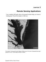
Water Models

GIS saves time and money in developing water distribution system
hydraulic models for simulating flows and pressures in the system.
GIS also helps in presenting the model results to non-technical
audiences.

EPANET and ArcView GIS integration.

2097_C012.fm Page 225 Monday, December 6, 2004 6:07 PM
Copyright © 2005 by Taylor & Francis



LEARNING OBJECTIVE

The learning objective of this chapter is to understand how GIS can be applied in
developing water distribution system hydraulic models and presenting the results
of the hydraulic models.

MAJOR TOPICS

• Development of hydraulic models
• Software examples
• EPANET model

• Network simplification (skeletonization)
• Estimation of node demands
• Estimation of node elevations
• Delineation of pressure zones
• Mapping the model output results
• GIS application examples and case studies

LIST OF CHAPTER ACRONYMS

AM/FM/GIS

Automated Mapping/Facilities Management/Geographic Information System

CIS

Customer Information System

COM

Component Object Model

COTS

Commercial Off-the-Shelf

DEM

Digital Elevation Model

DHI

Danish Hydraulic Institute

DLL

Dynamic Link Library

DRG

Digital Raster Graphic

GEMS

Geographic Engineering Modeling Systems

MMS

Maintenance Management System

ODBC

Open Database Connectivity

PRV

Pressure Regulating Valve

SCADA

Supervisory Control and Data Acquisition

TIF

Tag Image File

CITY OF GERMANTOWN’S WATER MODEL

The City of Germantown (Tennessee) water distribution system serves 40,000
people through 12,000 installations in a 17.5 mi

2

area. The system has approximately
95,000 ft of water pipes.

Application Water distribution system mapping and modeling
GIS software ArcGIS, ArcGIS Water Utilities Data Model (formerly
ArcFM Water Data Model), and MapObjects
Other software WaterCAD
GIS layers Digital orthophotos, pipes, hydrants, valves, manholes,
pumps, meters, fittings, sampling stations, and monitoring wells
Hardware Two Dell Precision 220 computers
Study area City of Germantown, Tennessee
Organization City of Germantown, Tennessee

2097_C012.fm Page 226 Monday, December 6, 2004 6:07 PM
Copyright © 2005 by Taylor & Francis

The City used ESRI’s geodatabase, an object-oriented GIS data model, to design a
database. The database design was done with minimal customization of ESRI’s ArcGIS
Water Utilities Data Model. This approach helped complete the database design in a
few weeks instead of several months. ESRI’s MapObjects was used to create a custom
utility tool set for developing the water distribution network. Valve and hydrant locations
from the digital orthophotos and planimetric mapping were used with the existing1in.

=

500 ft-scale paper map of the water system as the basis for connecting water pipes.
The GIS layers (Figure 12.1) were initially developed using the ArcView Shape-
files. The Shapefiles were then migrated to a geodatabase. To ease the data migration,
connectivity rules were stored in ArcCatalog rather than directly in the model.
ArcMap “flag and solver” tracing tools were used to ensure topological integrity of
the migrated data. ArcMap also provided the City with out-of-the-box network
analysis functionality such as tracing paths and water main isolation.
For the development of the hydraulic model, the City did not have to create a
modeling network from scratch. GIS was used to skeletonize the network for input
to the Haestad Method’s WaterCAD 4.1 hydraulic model. Spatial operations available
in ArcGIS were used to assign customer-demand data — obtained from the City’s
billing database and stored in parcel centroids — to modeling nodes. Node elevations
were extracted from the City’s DEM.
The hydraulic model was run to assess the future system expansion and capital
improvement needs of the City. The model indicated that the system needed a new
elevated storage tank and a larger pipe to deliver acceptable pressure under peak
demand conditions (ESRI, 2002b).

GIS APPLICATIONS FOR WATER DISTRIBUTION SYSTEMS

GIS has wide applicability for water distribution system studies. Representation

and analysis of water-related phenomena by GIS facilitates their management. The
GIS applications that are of particular importance for water utilities include mapping,
modeling, facilities management, work-order management, and short- and long-term
planning. Additional examples include (Shamsi, 2002):

• Conducting hydraulic modeling of water distribution systems.
• Estimating node demands from land use, census data, or billing records.
• Estimating node elevations from digital elevation model (DEM) data.
• Performing model simplification or skeletonization for reducing the number of
nodes and links to be included in the hydraulic model.
• Conducting a water main isolation trace to identify valves that must be closed to
isolate a broken water main for repair. Identifying dry pipes for locating customers
or buildings that would not have any water due to a broken water main. This
application is described in Chapter 15 (Maintenance Applications).
• Prepare work orders by clicking on features on a map. This application is described
in Chapter 14 (AM/FM/GIS Applications).
• Identifying valves and pumps that should be closed to isolate a contaminated part
of the system due to acts of terrorism. Recommending a flushing strategy to clean
the contaminated parts of the system. This application is described in Chapter 16
(Security Planning Vulnerability Assessment).

2097_C012.fm Page 227 Monday, December 6, 2004 6:07 PM
Copyright © 2005 by Taylor & Francis



• Providing the basis for investigating the occurrence of regulated contaminants
for estimating the compliance cost or evaluating human health impacts (Schock
and Clement, 1995).
• Investigating process changes for a water utility to determine the effectiveness

of treatment methods such as corrosion control or chlorination.
• Assessing the feasibility and impact of system expansion.
• Developing wellhead protection plans.

Figure 12.1

Germantown water distribution system layers in ArcGIS.

2097_C012.fm Page 228 Monday, December 6, 2004 6:07 PM
Copyright © 2005 by Taylor & Francis



By using information obtained with these applications, a water system manager
can develop a detailed capital improvement program or operations and maintenance
plan (Morgan and Polcari, 1991). The planning activities of a water distribution
system can be greatly improved through the integration of these applications.
In this chapter, we will focus on the applications related to hydraulic modeling
of water distribution systems.

DEVELOPMENT OF HYDRAULIC MODELS

The most common use of a water distribution system hydraulic model is to deter-
mine pipe sizes for system improvement, expansion, and rehabilitation. Models are also
used to assess water quality and age and investigate strategies for reducing detention
time. Models also allow engineers to quickly assess the distribution network during
critical periods such as treatment plant outages and major water main breaks.

Today, hydraulic models are also being used for vulnerability assessment and protection

against terrorist attacks.

Hydraulic models that are created to tackle a specific problem gather dust on a shelf
until they are needed again years later. This requires a comprehensive and often expen-
sive update of the model to reflect what has changed within the water system. A direct
connection to a GIS database allows the model to always remain live and updated.
Denver Water Department, Colorado, installed one of the first AM/FM/GIS
systems in the U.S. in 1986. In the early 1990s, the department installed the $60,000
SWS water model from the Stoner Associates (now Advantica Stoner, Inc.). Around
the same time, Genesee County Division of Water and Waste Services in Flint,
Michigan, started developing a countywide GIS database. The division envisioned
creating sewer and water layers on top of a base map and integrating the GIS layers
with their water and sewer models (Lang, 1992).
GIS applications reduce modeling development and analysis time. GIS can be used
to design optimal water distribution systems. An optimal design considers both cost-
effectiveness and reliability (Quimpo and Shamsi, 1991; Shamsi, 2002a) simulta-
neously. It minimizes the cost of the system while satisfying hydraulic criteria (accept-
able flow and pressures). Taher and Labadie (1996) developed a prototype model for
optimal design of water distribution networks using GIS. They integrated GIS for
spatial database management and analysis with optimization theory to develop a com-
puter-aided decision support system called WADSOP (Water Distribution System Opti-
mization Program). WADSOP employed a nonlinear programming technique as the
network solver, which offers certain advantages over conventional methods such as
Hardy-Cross, Newton Raphson, and linear system theory for balancing looped water
supply systems. WADSOP created a linkage between a GIS and the optimization model,
which provided the ability to capture model input data; build network topology; verify,
modify, and update spatial data; perform spatial analysis; and provide both hard-copy
reporting and graphical display of model results. The GIS analysis was conducted in
PC ARC/INFO. The ROUTE and ALLOCATE programs of the NETWORK module

2097_C012.fm Page 229 Monday, December 6, 2004 6:07 PM
Copyright © 2005 by Taylor & Francis



of PC ARC/INFO were found to be very helpful. Computational time savings of 80
to 99% were observed over the other programs.
Generally, there are four main tasks in GIS applications to water system
modeling:

1. Synchronize the model’s network to match the GIS network.
2. Transfer the model input data from a GIS to the model.
3. Establish the model execution conditions and run the model.
4. Transfer the model output results to GIS.

As described in Chapter 11 (Modeling Applications), GIS is extremely useful
in creating the input for hydraulic models and presenting the output. A hydraulic
modeler who spends hundreds of hours extracting input data from paper maps can
accomplish the same task with a few mouse clicks inside a GIS (provided that the
required data layers are available). GIS can be used to present hydraulic modeling
results in the form of thematic maps that are easy for nontechnical audiences to
understand. Additional information about GIS integration methods is provided in
Chapter 11, which provided a taxonomy developed by Shamsi (1998, 1999) to
define the different ways a GIS can be linked to hydraulic models. According to
Shamsi’s classification, the three methods of developing GIS-based modeling appli-
cations are interchange, interface, and integration. For GIS integration of water
distribution system hydraulic models, one needs a hydraulic modeling software
package. The software can run either inside or outside the GIS. As explained in
Chapter 11, when modeling software is run inside a GIS, it is considered “seam-
lessly integrated” into the GIS. Most modeling programs run in stand-alone mode

outside the GIS, in which case the application software simply shares GIS data.
This method of running applications is called a “GIS interface.”
The interchange method offers the most basic application of GIS in hydraulic
modeling of water distribution systems. In 1995, the Charlotte–Mecklenburg
Utility Department (CMUD) used this method to develop a KYPIPE model for
an area serving 140,000 customers from 2,500 mi of water pipes ranging in size
from 2 in. to 54 in. (Stalford and Townsend, 1995). The modeling was started
by creating an AutoCAD drawing of all pipes 12 in. and larger. The pipes were
drawn as polylines and joined at the intersections. The AutoCAD drawing was
converted to a facilities management database by placing nodes at the hydraulic
intersections of the pipes, breaking the polylines as needed, adding extended
attributes to the polylines from the defined nodes, extracting this information into
external tables, and adding the nongraphical information to the tables. Then, by
using ArcCAD inside AutoCAD, coverages were created for the pipes and nodes,
which could be viewed inside ArcView. Although this method was considered
state-of-the-art in 1995, it is not a very efficient GIS integration method by today’s
standards. The EPANET integration case study presented later in the chapter
exemplifies application of the more efficient integration method.
In the simplest application of the integration method, it should be possible to use
a GIS to modify the configuration of the water distribution network, compile model
input files reflecting those changes, run the hydraulic model from within the GIS, use
the GIS to map the model results, and graphically display the results of the simulation

2097_C012.fm Page 230 Monday, December 6, 2004 6:07 PM
Copyright © 2005 by Taylor & Francis



on a georeferenced base map. The integration method interrelationships among the
user, the hydraulic model, and the GIS software are illustrated in Figure 12.2.

SOFTWARE EXAMPLES

Table 12.1 lists representative water distribution system modeling packages and
their GIS capabilities, vendors, and Web sites. The salient GIS features of these
programs are described in the following subsections.

EPANET

EPANET was developed by the Water Supply and Water Resources Division
(formerly the Drinking Water Research Division) of the U.S. Environmental Pro-
tection Agency’s National Risk Management Research Laboratory (Rossman,
2000). It is a public-domain software that may be freely copied and distributed.
EPANET is a Windows 95/98/2K/NT program that performs extended-period
simulation of hydraulic and water quality behavior within pressurized pipe networks.
A network can consist of pipes, nodes (pipe junctions), pumps, valves, and storage
tanks or reservoirs. EPANET tracks the flow of water in each pipe, the pressure at
each node, the height of water in each tank, and the concentration of a chemical species

Figure 12.2

Integration method interrelationships.

2097_C012.fm Page 231 Monday, December 6, 2004 6:07 PM
Copyright © 2005 by Taylor & Francis



throughout the network during a simulation period made up of multiple time steps. In
addition to chemical species, water age and source tracing can also be simulated.

The Windows version of EPANET provides an integrated environment for editing
network input data, running hydraulic and water quality simulations, and viewing the
results in a variety of formats. These include color-coded network maps, data tables,
time-series graphs, and contour plots. Figure 12.3 shows an EPANET screenshot dis-
playing pipes color-coded by head-loss and nodes color-coded by pressure.
The EPANET Programmer’s Toolkit is a dynamic link library (DLL) of functions
that allow developers to customize EPANET’s computational engine for their own
specific needs. The functions can be incorporated into 32-bit Windows applications
written in C/C++, Delphi Pascal, Visual Basic, or any other language that can call
functions within a Windows DLL. There are over 50 functions that can be used to open
a network description file, read and modify various network design and operating
parameters, run multiple extended-period simulations accessing results as they are
generated or saving them to file, and write selected results to file in a user-specified
format. The toolkit should prove useful for developing specialized applications,
such as optimization models or automated calibration models, that require running
many network analyses while selected input parameters are iteratively modified.
It also can simplify adding analysis capabilities to integrated network modeling envi-
ronments based on CAD, GIS, and database management packages (Rossman, 2000a).
The current version of EPANET (Version 2.0) has neither a built-in GIS interface nor
integration. Therefore, users must develop their own interfaces (or integration) or rely on
the interchange method to manually extract model input parameters from GIS data layers.

H

2

ONET

™

and H

2

OMAP

™

MWH Soft, Inc. (Broomfield, Colorado), provides infrastructure software and
professional solutions for utilities, cities, municipalities, industries, and engineering
organizations. The company was founded in 1996 as a subsidiary of the global

Table 12.1

Water Distribution System Modeling Software
Software Method Vendor Web site

EPANET Interchange U.S. Environmental
Protection Agency
(EPA)
www.epa.gov/ord/NRMRL/
wswrd/epanet.html
AVWater Integration CEDRA Corporation www.cedra.com
H

2

ONET and
H

2

OMAP
Interface and
Integration
MWH Soft www.mwhsoft.com
InfoWorks WS
and InfoNet
Interface and
Integration
Wallingford Software www.wallingfordsoftware.com
MIKE NET Interface DHI Water &
Environment
www.dhisoftware.com
PIPE2000 Pro Interface University of
Kentucky
www.kypipe.com
SynerGEE
Water
Interface and
Integration
Advantica Stoner www.stoner.com
WaterCAD Interface Haestad Methods www.haestad.com
WaterGEMS Integration

2097_C012.fm Page 232 Monday, December 6, 2004 6:07 PM
Copyright © 2005 by Taylor & Francis

environmental engineering, design, construction, technology, and investment firm
MWH Global, Inc. The company’s CAD- and GIS-enabled products are designed
to manage, design, maintain, and operate efficient and reliable infrastructure systems.
MWH Soft, provides the following water distribution system modeling software:

•H

2

ONET
•H

2

OMAP Water
• InfoWater
•H

2

OVIEW Water

H

2

ONET is a fully integrated CAD framework for hydraulic modeling, network
optimization, graphical editing, results presentation, database management, and
enterprise-wide data sharing and exchange. It runs from inside AutoCAD and,
therefore, requires AutoCAD installation.

Figure 12.3

EPANET screenshot (Harrisburg, Pennsylvania, model).

2097_C012.fm Page 233 Monday, December 6, 2004 6:07 PM
Copyright © 2005 by Taylor & Francis



Built using the advanced object-oriented geospatial component model, H

2

OMAP
Water provides a powerful and practical GIS platform for water utility solutions. As
a stand-alone GIS-based program, H

2

OMAP Water combines spatial analysis tools
and mapping functions with network modeling for infrastructure asset management
and business planning. H

2

OMAP Water supports geocoding and multiple mapping
layers that can be imported from one of many data sources including CAD drawings
(e.g., DWG, DGN, and DXF) and standard GIS formats (Shapefiles, Generate files,
MID/MIF files, and ArcInfo coverages). The program also supports the new geoda-

tabase standard of ArcGIS through an ArcSDE connection.
InfoWater is a GIS-integrated water distribution modeling and management
software application. Built on top of ArcGIS using the latest Microsoft .NET and
ESRI ArcObjects component technologies, InfoWater integrates water network mod-
eling and optimization functionality with ArcGIS.
H

2

OVIEW Water is an ArcIMS-based (Web-enabled) geospatial data viewer and
data distribution software. It enables deployment and analysis of GIS data and
modeling results over the Internet and intranets. Figure 12.4 shows a screenshot of
H

2

OVIEW Water.
Various GIS-related modules of H

2

O products are described in the following
subsections.

Figure 12.4

H

2

OVIEW screenshot (Screenshot courtesy of MWH Soft).

2097_C012.fm Page 234 Monday, December 6, 2004 6:07 PM
Copyright © 2005 by Taylor & Francis



Demand Allocator

Automatically computes and geographically allocates water demand data
throughout the water distribution network model.

Skeletonizer

Automates GIS segmentation (data reduction, skeletonization, and trimming) to con-
struct hydraulic network models and reallocates node demands directly from the GIS.

Tracer

H

2

ONET Tracer is a network tracing tool that locates all valves which need to
be closed to isolate a portion of the network, visually identify all customers affected
by loss or reduction in service, and determine the best response strategy. It is a
valuable tool for vulnerability analysis and security planning to protect systems
against terrorist attacks.

WaterCAD

™

and WaterGEMS

™

Haestad Methods, Inc. (Waterbury, Connecticut), provides a wide range of H&H
computer models, publishes books, and offers continuing education for the civil
engineering community. Haestad Methods is a growing company with more than
100,000 users in more than 160 countries around the world. Haestad Methods was
acquired by Bentley Systems (Exton, Pennsylvania) in August 2004. Provides the
following water distribution system modeling software:

• WaterCAD Stand-alone
• WaterCAD for AutoCAD
• WaterGEMS for ArcGIS

WaterCAD is Haestad Method’s water distribution analysis and design tool. It
can analyze water quality, determine fire flow requirements, and calibrate large
distribution networks. The stand-alone version does not require a CAD or GIS
package to run. The AutoCAD version runs from inside AutoCAD and, therefore,
requires AutoCAD.
Shapefile Wizard, the ArcView GIS interface module for WaterCAD, is sold
separately. The wizard provides import and export capability to transfer data between
GIS and WaterCAD models. For example, Import Shapefile Wizard imports Water-
CAD model input parameters from ArcView GIS Shapefiles. Similarly, the Export
Shapefile Wizard exports hydraulic model networks to ArcView. This feature lets
users build and maintain their water and sewer networks directly inside a GIS.
Geographic Engineering Modeling Systems (GEMS) is the next generation of

Haestad Methods’ hydraulic network modeling products. GEMS is a new product

2097_C012.fm Page 235 Monday, December 6, 2004 6:07 PM
Copyright © 2005 by Taylor & Francis



family that combines water, wastewater, and stormwater system modeling with an open
database architecture. It was developed using ESRI’s ArcObjects technology and com-
puting tools from Microsoft’s .NET initiative. GEMS technology eliminates the need
for a separate model database. It streamlines the process of accessing information on,
for example, facilities management, zoning, topography, and gauging stations for use
with the model. GEMS-based models can be run within ESRI’s ArcGIS software using
the geodatabase structure (Shamsi, 2001).
WaterGEMS uses a geodatabase, Water Data Model, for integrated WaterCAD
modeling within the ArcGIS platform. Because WaterGEMS runs from inside ArcGIS,
it requires an installation of ArcGIS software. Although WaterGEMS accommodates
Shapefiles and ArcInfo coverages, it provides users with the tools to migrate to the new
geodatabase format. Users can easily save an existing hydraulic model as a geodatabase.
In an interview by Haestad Methods, Jack Dangermond, president of ESRI,
stated, “GEMS bridges the gap between engineering and planning departments and
allows users to further leverage their GIS investment” (Haestad Methods, 2003).

MIKE NET

™

DHI Water and Environment (formerly Danish Hydraulic Institute, Hørsholm,
Denmark, www.dhi.dk) is a global provider of specialized consulting and numerical
modeling software products for water, wastewater, river and coastal engineering,

and water resources development. DHI has developed a large number of hydraulic,
hydrologic, and hydrodynamic computer models for water, wastewater, and storm-
water systems. The company also specializes in linking its computer models with
GIS so that modelers can use both modeling and GIS technologies within a single
product. Since 1998, DHI has embarked on an ambitious program to link its models
with the ESRI family of GIS products. Many of DHI’s modeling systems now support
GIS data transfer. For example, DHI has developed ArcView GIS extensions and
interface programs for a number of its products.
MIKE NET is a software package for the simulation of steady flow and pressure
distribution and extended-period simulation of hydraulic and water quality behavior
within drinking water distribution systems. MIKE NET was developed in coopera-
tion with BOSS International (Madison, Wisconsin, www.bossintl.com). MIKE NET
uses the EPANET 2.0 numerical engine.
Data can be shared with any standard Windows spreadsheet (e.g., Microsoft
Excel) or relational database (e.g., Oracle, Microsoft SQL Server, Informix, and
Sybase) either directly or using Open Database Connectivity (ODBC) links, or by
simply cutting to and pasting from the Microsoft Windows clipboard.
Important GIS features of MIKE NET are described below:

• MIKE NET can read the network models directly from an ArcInfo, ArcFM,
ArcView, or MapInfo GIS database. MIKE NET can build a link to a GIS
database structure, using attribute mapping and geocoding. For example, a pump
or valve can be represented as either a node or an arc in the originating GIS
database, while still being linked with MIKE NET.
• MIKE NET can read the node elevation field from Shapefile polygons and assign
it to each junction node within the polygon.

2097_C012.fm Page 236 Monday, December 6, 2004 6:07 PM
Copyright © 2005 by Taylor & Francis

• MIKE NET can import a fire hydrants layer to automatically determine which
pipe the hydrant belongs to. It temporarily inserts the hydrant into the pipe at the
hydrant location, performs the fire flow simulation, and resets the network back
to the original state without the hydrant.
• MIKE NET allows the user to assign nodal demands to the entire network system
using the program’s Distributed Demands capability. In addition, GIS layers can
be used to geocode water consumption as well as multiple demand patterns from
land-use and population-density aerial coverages. Multiple overlying layers can
be aggregated and assigned to the appropriate junction nodes.
• It can perform automated and/or user-assisted skeletonization of the distribution
network. Node demands are automatically accumulated during the skeletonization
process so that the skeletal model continues to perform and respond closely to
those of the original network model.

Other Programs

CEDRA AVWater from Cedra Corporation (Rochester, New York) provides an
ArcView 3.x GIS extension interface to the University of Kentucky’s KYPIPE and
EPA’s EPANET models.
The InfoWorks WS from Wallingford Software (Wallingford, United Kingdom)
imports models from any data source using the InfoWorks CSV data gateway. It
exchanges data with MapInfo Professional and ArcView GIS and exports data and
simulation results to MapInfo Professional and ArcView. InfoNet has a multiuser
database with built-in data models for water, wastewater, and stormwater infrastruc-
ture; a GIS user-interface; and a report generator. It can be integrated with GIS,
Desktop Office systems, hydraulic modeling systems, maintenance management
systems (MMS), field data systems, SCADA, and corporate databases.
PIPE2000 is the hydraulic modeling software from the developers of the legacy

KYPIPE program from the University of Kentucky (Lexington, Kentucky).
PIPE2000 uses the EPANET simulation engine for water quality simulation. The
Pro version of PIPE2000 imports and exports PIPE2000 data to and from Shapefiles.
SynerGEE Water (formerly Stoner Model) is a hydraulic modeling software from
Stoner Advatica, Inc. (Carlisle, Pennsylvania). Water Solver uses SynerGEE’s sim-
ulation engine as a Microsoft Component Object Model (COM)-compliant compo-
nent. This capability allows integration of hydraulic simulation capability into a GIS.

EPANET AND ARCVIEW INTEGRATION IN HARRISBURG

A representative example of model integration is presented in this section.
Additional water system modeling case studies are provided in Chapter 17 (Appli-
cations Sampler).
Chester Engineers (Pittsburgh, Pennsylvania) developed a GIS integrated
model by combining ESRI’s ArcView GIS software and EPA’s EPANET hydraulic
modeling program (Maslanik and Smith, 1998). EPANET provides extensive
capability to support decisions in the operation, management, planning, and
expansion of water distribution systems. ArcView is a user-friendly desktop

2097_C012.fm Page 237 Monday, December 6, 2004 6:07 PM
Copyright © 2005 by Taylor & Francis



mapping and GIS tool, which can be learned by most users without extensive
training and experience. Due to its low cost, ease of use, and customization
capability, ArcView was found to be a suitable tool for developing the EPA-
NET–GIS integration.
The custom ArcView 3.x and EPANET 2.x integration is called AVNET. AVNET
performs preprocessing of GIS data to create model input files. It also conducts

postprocessing of model results to create GIS maps of the model output results.
Both the GIS and the modeling functions are available in ArcView. There is no need
to exit ArcView to edit or run the model. AVNET provides seamless model input
creation, model data editing, model execution, and model output display capabilities
from within ArcView GIS. Other important features of AVNET are:

• As shown in the figure on the first page of this chapter, AVNET adds a new
EPANET menu to ArcView’s standard interface. The AVNET menu provides eight
functions listed in Table 12.2.
• As shown in Figure 12.5, AVNET adds three new editing tools to ArcView’s
standard interface. These tools provide three functions listed in Table 12.2. These
CAD-like editing tools allow adding nodes and pipes and on-screen input of model
attributes.
• AVNET uses ArcView to modify the configuration of the water distribution system.
• Water mains and links can be added interactively while maintaining the required
network topology.
• AVNET compiles new EPANET model input files reflecting the edits made by
the user.
• AVNET requires ArcView Shapefiles or ArcInfo coverages for nodes and pipes.
The required attributes for these layers are shown in Table 12.3.

Table 12.2

AVNET Functions
Function Description

Menu Functions

Set Environment Enter model execution parameters (e.g., length of
simulation)

Make Input Makes EPANET input file
Run EPANET Launches the EPANET program
Results Read Translates the EPANET output file into GIS
database files
Model Min/Max Finds the minimum and maximum
EPANET output parameters
Results Join Joins the EPANET results for a selected
hour or minimum/maximum values to a layer
Results View Sets the legend to an EPANET output parameter
Remove Results Removes the join of the EPANET results
from a theme

Tool Functions

N Tool Adds a water system node
L Tool Adds a water system main
S Tool Splits an existing water system line and adds a
node

2097_C012.fm Page 238 Monday, December 6, 2004 6:07 PM
Copyright © 2005 by Taylor & Francis



Table 12.3

AVNET Attributes
Attribute Type Description

Attributes for the Node Layer

Node Numeric Node ID number
X_coord Numeric X coordinate value
Y_coord Numeric Y coordinate value
Type Character Node type (JUNCTION or TANK)
Elev Numeric Node elevation
Demand Numeric Node demand (water consumption)
Init_level Numeric Initial level of water system tank
Min_level Numeric Minimum level of water system tank
Max_level Numeric Maximum level of water system tank
Diam Numeric Diameter of water system tank

Attributes for the Pipe Layer

Link Numeric Line ID
Start_node Numeric Node ID number of starting node of pipe
End_node Numeric Node ID number of ending node of pipe
Type Character Main type (PIPE or PUMP)
Length Numeric Pipe length
Diam Numeric Pipe diameter
Rough_coef Numeric Pipe roughness coefficient
Pump_H Numeric Pump design head
Pump_Q Numeric Pump design flow

Figure 12.5

Editing pipe attributes in AVNET model.

2097_C012.fm Page 239 Monday, December 6, 2004 6:07 PM
Copyright © 2005 by Taylor & Francis

Figure 12.6

Reading the EPANET model output results in ArcView GIS.

Figure 12.7

Classifying the legend to create model output thematic maps.

2097_C012.fm Page 240 Monday, December 6, 2004 6:07 PM
Copyright © 2005 by Taylor & Francis



• AVNET creates a map file for EPANE model that contains a line for each node
with the node ID and the x and y coordinates. The data are extracted from the
water system node attribute table.
• AVNET runs the EPANET model from within ArcView.
• AVNET uses ArcView to map the water distribution system model and graphically
display the results of the simulation on a georeferenced base map. The output file
is linked to the GIS attribute files for pipes and nodes. As shown in Figure 12.6,
AVNET reads the output file to extract the output parameters for minimum and
maximum values or values at any user-specified simulation time step. Thematic
maps of model output parameters (flows, pressures, residual chlorine, etc.) are
created by classifying the ArcView theme legends (Figure 12.7).
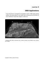
Figure

12.8 shows the AVNET model for the city of Harrisburg, Pennsylvania.

This model consists of 2500 pipes and 1650 nodes, 4 tanks, and 6 pumps. It
shows layers for model nodes and links (pipes). The base-map layer consists of
a USGS digital raster graphic (DRG) layer. A DRG is a TIF file of a scanned
USGS 7.5-min paper topographic map.

Figure 12.8

AVNET model for the City of Harrisburg, Pennsylvania.

2097_C012.fm Page 241 Monday, December 6, 2004 6:07 PM
Copyright © 2005 by Taylor & Francis



Mapping the Model Output Results

The power of GIS gives a new meaning to the popular phrase “a picture is worth a
thousand words.” In fact, the thematic maps created by GIS are so effective in displaying
large amounts of complex data that the popular phrase can be “plagiarized” to create a

new cliché “a map is worth a thousand numbers.”

The model output results in tabular or spreadsheet format are not very
meaningful for nonmodelers. GIS technology is an effective means of bridging
the gap between modeling information and its recipients. GIS can convert
textual output results into easily

interpretable

thematic maps, for example, a map

of pipes color-coded by flows and nodes color-coded by pressures.

Figure 12.9

shows the Harrisburg model output results presented as a thematic map in ArcView
GIS. The first layer (represented as dots) shows the minimum working pressures
at the nodes. The second layer (represented as lines) shows the maximum head
losses for the pipes. An overlay of the two layers clearly shows areas where
pressures are low and head losses high. Such areas usually represent inadequate
pipe sizes for delivering required flow rates and might be targeted for water main
installation and replacement work. In fact, the GIS can automatically flag such
hot spots for further study. The model output thematic maps are excellent for
conveying modeling results to nontechnical audiences such as members of the city
council or water utility board, or the general public.

Figure 12.9

EPANET output results presented as a map in ArcView GIS.

2097_C012.fm Page 242 Monday, December 6, 2004 6:07 PM
Copyright © 2005 by Taylor & Francis



NETWORK SKELETONIZATION

GIS and CAD layers of water distribution systems often have a level of detail that
is unnecessary for analyzing system hydraulics. This can include hydrants, service
connections, valves, fittings, and corner nodes. Although development of models that
are an exact replica of the real system is now possible due to enormously powerful

computers, the cost of purchasing, developing, and running very large models can be
excessive. Attempting to include all the network elements could be a huge undertaking
that may not have a significant impact on the model results (Haestad Methods, 2003).
Modelers, therefore, resort to a network simplification process, which is also referred
to as the “skeletonization” process.
Network simplification is needed to increase processing speed without compro-
mising model accuracy. Manual skeletonization is a cumbersome process. Modelers,
therefore, have resorted to rules-of-thumb, such as excluding all pipes smaller than
a certain size. This approach requires a significant effort in locating and removing
the candidate pipes. In addition, the network integrity



and connectivity might be
adversely impacted, with a potential to alter the output results significantly.
An example of how GIS performs skeletonization is shown in

Figure 12.10

to

Figure 12.16.



Figure 12.10

shows a portion of the water distribution system of the city
of Sycamore, Illinois. It shows the GIS layers for parcels, water mains, service lines,
service valves, distribution system valves, and fire hydrants. If a modeling node is

created at each pipe junction, valve, and hydrant, the resulting network model (shown
in

Figure 12.11

) would have 93 nodes and 94 pipes (links). If this process is extended
to the entire system, we could expect thousands of nodes and pipes. For large

Figure 12.10

GIS layers for the Sycamore water distribution system.

2097_C012.fm Page 243 Monday, December 6, 2004 6:07 PM
Copyright © 2005 by Taylor & Francis



systems, this process can generate several hundred thousand nodes and pipes.
Skeletonization can be performed in a GIS using the following steps:

1. It is not necessary to create nodes at the fire hydrants because fire flow demand
can be modeled at a nearby node. Thus, nodes corresponding to fire hydrants
can be eliminated without compromising the modeling accuracy. Figure 12.12
shows the resulting skeletonized network with 86 nodes and 87 pipes. This
represents an 8% reduction in the number of nodes and pipes.
2. It is not necessary to create nodes at all the distribution system valves. For
example, the effect of an isolation valve (e.g., gate valves and butterfly valves)
can be modeled as part of a pipe by using minor loss coefficients. In some
models, closed valves and check valves can be modeled as links. Thus, nodes
corresponding to most valves can be eliminated without compromising mod-

eling accuracy. Figure 12.13 shows the skeletonized network after removing
the valve nodes. It now has 81 nodes and 82 pipes representing a 13% reduction
in the number of original nodes and pipes. This level of skeletonization is
considered minimum.
3. It is not necessary to model corner nodes that describe actual layout of pipes.
The pipe layout does not affect model output as long as the pipe length is
accurate. Any potential head loss due to sharp turns and bends can be modeled
using minor loss coefficients or friction factors. Thus, nodes corresponding to
corner nodes can be eliminated without compromising modeling accuracy.
Figure 12.14 shows the skeletonized network after removing the corner nodes.
It now has 78 nodes and 79 pipes, representing a 16% reduction in the number
of original nodes and pipes.

Figure 12.11

Network model without skeletonization.

2097_C012.fm Page 244 Monday, December 6, 2004 6:07 PM
Copyright © 2005 by Taylor & Francis



Figure 12.12

Skeletonized network model after removing nodes at fire hydrants.

Figure 12.13

Skeletonized network model after removing nodes at valves.

2097_C012.fm Page 245 Monday, December 6, 2004 6:07 PM
Copyright © 2005 by Taylor & Francis



Figure 12.14

Skeletonized network model after removing corner nodes.

Figure 12.15

Skeletonized network model after removing pipes less than 8 in.

2097_C012.fm Page 246 Monday, December 6, 2004 6:07 PM
Copyright © 2005 by Taylor & Francis



4. Small pipes with low flows can also be eliminated without significantly changing
the modeling results. There are no absolute criteria for determining which pipes
should be eliminated (Haestad et al., 2003). Elimination of pipes less than 6 in.
or 8 in. is most common. Thus, small pipes and corresponding nodes can be
eliminated for further network simplification. Figure 12.15 shows the skeletonized
network after removing pipes of less than 8 in. width. The most dramatic effect of
this step is the removal of all the service lines from the network model. The network
now has 36 nodes and 41 pipes, representing a 56% reduction in the number of
original nodes and pipes. This moderate level of skeletonization is acceptable in most
cases.
5. Further reduction in the size of a network model is possible by aggregating the
demands from several customers to a single node. Figure 12.16 shows the skele-

tonized network after dividing the network into three demand zones and assigning
the total zone demand to a node inside that zone. The network now has only 3
nodes and 5 pipes, representing a 96% reduction in the number of original nodes
and a 94% reduction in the number of original pipes. This high level of skeleton-
ization can affect modeling results. For example, this model cannot model the
flows and pressures at different houses within the subdivision.

Although the preceding steps can be performed manually in a GIS by editing
the data layers, the process will be too cumbersome unless the system is very small.
Automatic GIS-based skeletonization that can be completed quickly is now avail-
able in some software packages. Automatic skeletonization removes the complexity
from the data, while maintaining the network integrity and hydraulic equivalency
of the system. Reductions of 10 to 50% in the size of a network are possible. These
programs allow the users to input the skeletonization criteria such as the smallest

Figure 12.16

Skeletonized network model after aggregating demand nodes.

2097_C012.fm Page 247 Monday, December 6, 2004 6:07 PM
Copyright © 2005 by Taylor & Francis



Figure 12.17

Skeletonizer’s network simplification results. Top: original system with 2036
pipes. Bottom: skeletonized network with 723 pipes (65% reduction). (Maps
courtesy of MWH Soft, Inc.)

2097_C012.fm Page 248 Monday, December 6, 2004 6:07 PM
Copyright © 2005 by Taylor & Francis



pipe size that should be included in the model. The smallest-pipe-size criterion
should be used carefully because both size and accuracy of the skeletonized model
depend on it. A highly skeletonized model does not work well in areas where most
of the water supply is through small pipes.
The Skeletonizer

™

module of H

2

OMap water system modeling software
(MWH Soft, Inc., Broomfield, Colorado, www.mwhsoft.com) and Skelebrator

™

module of WaterCAD and WaterGEMS water system modeling software (Haestad
Methods, Waterbury, Connecticut, www.haestad.com) are examples of software
tools that automate the skeletonization of CAD and GIS layers.
Figure 12.17 shows
an example of Skeletonizer skeletonization. The top screenshot shows the original
network with 2036 pipes imported from a GIS. The bottom screenshot shows the
skeletonized network with 723 pipes, indicating a 65% reduction in the size of
the network.

Mohawk Valley Water (MVW) is a water utility serving more than 125,000
people in approximately 150 mi
2
area in central New York. In 2002, MVW created
an all-pipe WaterCAD hydraulic model that was connected to a geodatabase. A
reduce/skeletonize/trim (RST) process was used to eliminate hydrant laterals and
private service connections to scale the hydraulic model to pipe segments 4-in. and
greater. The demands, pipe attributes, and elevations were extracted from the geo-
database (DeGironimo and Schoenberg, 2002).
ESTIMATION OF NODE DEMANDS
Node demand is an important input parameter of a hydraulic model, representing
the water consumption rate in units of volume/time (e.g., gallons per day or liters per
second). Demands are grouped by customer type (e.g., residential, commercial, indus-
trial, or institutional) or magnitude (e.g., average daily, maximum daily, peak hourly,
or fire flow). Manual estimation of node demands from customer billing records is a
cumbersome process. Modelers, therefore, have traditionally resorted to approximate
methods, such as uniform distribution of the residential water use across all nodes
followed by adding the nearest commercial and industrial use at various nodes. This
approach requires a significant effort in fine-tuning the node demands during the
model calibration phase of the project.
GIS allows implementation of more accurate demand estimation methods. One
such method utilizes the GIS to geocode (or geolocate) all individual water users
(defined by the address at which each meter is located) and to assign the metered
water consumption rates for each meter location to the nearest node in the model.
The geocoding process links a street address to a geographic location and finds the
coordinates of a point location based on its street address. This method assumes that
a computer file (spreadsheet or delimited text file) containing meter addresses and
metered water use for specified durations (e.g., quarterly or monthly) can be pro-
duced from the utility’s billing database. If this information is available, the following
procedure can be used to assign demands to nodes:

2097_C012.fm Page 249 Monday, December 6, 2004 6:07 PM
Copyright © 2005 by Taylor & Francis