Handbook of Ecological Indicators for Assessment of Ecosystem Health - Chapter 3 docx
Bạn đang xem bản rút gọn của tài liệu. Xem và tải ngay bản đầy đủ của tài liệu tại đây (1.45 MB, 38 trang )
CHAPTER 3
Application of Ecological Indicators to
Assess Environmental Quality in Coastal
Zones and Transitional Waters:
Two Case Studies
J.C. Marques, F. Salas, J.M. Patrı
´
cio, and M.A. Pardal
This chapter addresses the application of ecological indicators in assessing
the biological integrity and environmental quality in coastal ecosystems and
transitional waters. In this context, the question of what might be considered a
good ecological indicator is approached, and the different types of data most
often utilized to perform estimations are discussed. Moreover, we present a brief
review on the application of ecological indicators in coastal and transitional
waters ecosystems referring to: (1) indicators based on species presence vs.
absence; (2) biodiversity as reflected in diversity measures; (3) indicators based
on ecological strategies; (4) indicators based on species biomass and abundance;
(5) indicators accounting for the whole environmental information; and
(6) thermodynamically oriented and network an alysis-based indicators.
Algorithms are provided in an abridged way and the pros and cons regarding
the application of each indicator are discussed. The question of how to choose
the most adequate indicator for each particular case is discussed as a function of
data requirements and data availability. Two case studies are used to illustrate
whether a number of selected ecological indicators were satisfactory in
describing the state of ecosystems, comparing their relative performances and
Copyright © 2005 by Taylor & Francis
discussing how their usage can be improved for environment health assessment.
The possible relation between values of these indicators and the environmental
quality status of ecosystems was analyzed. We reached the conclusion that to
select an ecological indicator, we must account for its dependence on external
factors beyond our control, such as the need for reference values that often do
not exist, or particular characteristics regarding the habitat type. As a result, it is
reasonable to say that no ind icator will be valid in all situations, and that a
single approach does not seem appropriate due to the complexity inherent in
assessing the environmental quality status of a system. Therefore, as a principle,
such evaluation should be always performed using several ecological indicators,
which may provide complementary information.
3.1 INTRODUCTION
Ecological indicators are commonly used to supply synoptic information
about the state of ecosystems. They usually address an ecosystem’s structure
and/or functioning accounting for a certain aspect or component; for example,
nutrient concentrations, water flows, macroinvertebrates and/or vertebrates
diversity, plants diversity, plants productivity, erosion symptoms, and
sometimes ecological integrity at a systems level.
The main attribute of an ecological indicator is to combine numerous
environmental factors in a single value, which might be useful in terms of
management and for making ecological concepts compliant with the general
public understanding. Moreover, ecological indicators may help in establishing
a useful connection between empirical research and modeling since some of
them are of use as orientors (also referred to in the literature as goal functions)
in ecological models. Such application proceeds from the fact that conven-
tional models of aqu atic ecosystems are not effective in predicting the
occurrence of qualitative changes in ecosystems; for example, shifts in species
composition, which is due to the fact that measurements typically carried
out — such as biomass and production — are not efficient at capturing such
modifications (Nielsen, 1995). Nevertheless, it has been tried to incorporate
this type of changes in structurally dynamic models (Jørgensen, 1992; Nielsen,
1992, 1994, 1995; Jørgensen et al., 2002), to improve their predictive capability,
achieving a better understanding of ecosystem behavior, and consequently a
better environmental management.
In structurally dynamic models, the simulated ecosystem behavior and
development (Nielsen, 1995; Stras
ˇ
kraba, 1983) is guided through an optimiza-
tion process by changing the model parameters in accordance with a given
ecological indicator, used as an orientor (goal function). In other words, this
allows the introduction in models parameters that change as a function of
changing forcing functions and conditions of state variables, optimizing the
model outputs by a stepwise approach. In this case, the orientor is assumed to
express a given macroscopic property of the ecosystem, resulting from the
emergence of new characteristics arising from self-organization processes.
68 HANDBOOK OF ECOLOGICAL INDICATORS FOR ASSESSMENT OF ECOSYSTEM HEALTH
Copyright © 2005 by Taylor & Francis
In general, the application of ecological indicators is not free from criticism.
One such criticism is that aggregation results in oversimplification of the
ecosystem unde r observation. Moreover, problems arise from the fact that
indicators account not only for numerous specific system characteristics, but
also other kinds of factors; for example, physical, biological, ecological, socio-
economic etc. Indicators must therefore be utilized following the right criteria
and in situations that are consistent with its intended use a nd scope; otherwise
they may lead to confusing data interpretations.
This paper addresses the application of ecological indicators for assessing
the biological integrity and environmental quality in coastal ecosystems and
transitional waters. The possible characteristics of a good ecological indicator,
or what kind of information regarding ecosystem responses can be obtained
from the different types of biological data usually taken into account in
evaluating the state of coastal areas, has already been discussed in chapter 2.
Two cases studies are used to illustrate whether different types of indicators
were satisfactory in describing the state of ecosystems, comparing their relative
performances and discussing how can their usage be improved for environment
health assessment.
3.2 BRIEF REVIEW ON THE APPLICATION OF ECOLOGICAL
INDICATORS IN ECOSYSTEMS OF COASTAL AND
TRANSITIONAL WATERS
Almost all coastal marine and transitional waters ecosystems all over the
world have been under severe environmental stress following the settlement of
human activities. Es tuaries, for example, are the trans ition between marine,
freshwater and land ecosystems, being characterized by distinctive biological
communities with specific ecological and physiological adaptations. In fact, we
may say that the estuarine habitat does not imply a simple overlap of marine
and land factors, constituting instead an individualized whole with its own
biogeochemical factors and cycles, which represents the environment for real
estuarine species to evolve. In such ecosystems, besides resources available,
fluctuating conditions, namely salinity and type of substrate, are a key issue
regarding an organism’s ecological distribution and adaptive strategies (see, for
example, McLusky, 1989; Engle et al., 1994).
The most common types of problems in terms of pollution include illegal
sewage discharges associated with nutrient enrichment; pollution due to toxic
substances such as pesticides, heavy metals, and hydrocarbons; unlimited
development; and habitat fragmentation or destruction.
In the case of transitional waters, limited water circulation and inappro-
priate water management tends to concentrate nutrients and pollutants, and
to a certain extent we may say that sea pollution begins there (Perillo et al.,
2001). Moreover, in estuaries, drainage of harbors and channels modifies
geomorphology, water circulation, and other physicochemical features, and
consequently the habitat’s characteristics. In recent times, perhaps the most
Copyright © 2005 by Taylor & Francis
important problem is the excessive loading of nutrients mainly due to fertilizers
used in agriculture, and untreated sewage water, which induces eutrophication
processes. These problems can be observed all over the world.
Many ecological indicators used or tested in evaluating the status of these
ecosystems can be found in the literature, resulting from just a few distinct
theoretical approaches. A number of them focus on the presence or absence of
given indicator species, while others take into account the different ecological
strategies carried out by organisms, diversity, or the energy variation in the
system through changes in the biomass of individuals. A last group of
ecological indicators are thermodynamically oriented or based on network
analysis, and look for capturing the information on the ecosystem from a more
holistic perspective (Table 3.1).
3.2.1 Indicators Based on Species Presence vs. Absence
Determining the presence or absence of one species or group of species has
been one of the most used approaches in detecting pollution effects. For
instance, the Bellan, (based on polychaetes), or the Bellan–Santini (based on
amphipods) indice s attempt to characterize environmental conditions by
analyzing the dominance of species that indicate some type of pollution in
relation to the species considered to indicate an optimal environmental
situation (Bellan, 1980; Bellan and Santini, 1980). Several authors do not
advise the use of these indicators because often such indicator species may
occur naturally in relative high densities. The point is that there is no reliable
methodology to know at which level the indicator species can be well
represented in a community that is not really affected by any kind of pollution,
which leads to a significant exercise of subjectivity (Warwick, 1993). Despite
these criticisms, even recently, the AMBI index (Borja et al., 2000), which is
based on the Glemarec and Hily (1981) species classification regarding
pollution; as well as the Bentix index (Simbora and Zenetos, 2002), have gone
back to update such pollution detecting tools. Roberts et al. (1998) also
proposed an index based on macrofauna species, which accounts for the ratio
of each species abundance in control vs. samples proceeding from stressed
areas. It is however semiquantitative as well as site- and pollution type-specific.
The AMBI index, for example, accounts for the presence of species
indicating a type of pollution and of specie s indicating a reference situation
assumed to be polluted. It has been considered useful in terms of the
application of the European Water Framework Directive in coastal ecosystems
and estuaries. In fact, although this index is very much based on the paradigm
of Pearson and Rosenberg (1978), which emphasizes the influence of organic
matter enrichment on benthic communities, it was shown to be useful in
assessing other anthropogenic impacts, such as physical alterations in the
habitat, heavy metal inputs, etc. in several European areas of the Atlantic
(North Sea; Bay of Biscay; and southern Spain) and Mediterranean coasts
(Spain and Greece) (Borja et al., 2003).
Copyright © 2005 by Taylor & Francis
Table 3.1 Short review of environmental quality indicators regarding the benthic communities
Type of indicator
Requirements and applicability
evaluation Algorithm
Based on species
presence vs. absence
List of species. Subjective in
most of the cases. Only the
use of AMBI and Bentix
is recommended.
Bellan index (Bellan, 1980):
IP ¼
X
pollution species indicator
no pollution species indicator
Pollution indicator species: Platenereis dumerilli,
Theosthema oerstedi, Cirratulus cirratus and Dodecaria concharum.
No-pollution indicator species: Syllis gracillis, Typosyllis prolifera,
Typosyllis sp. and Amphiglena mediterranea.
Bellan–Santini index (Bellan-Santini,1980):
IP ¼
X
pollution species indicator
no pollution species indicator
Pollution indicator species: Caprella acutrifans and Podocerus variegates
No-pollution indicator species: Hyale sp,
Elasmus pocillamunus and Caprella liparotensis
AMBI (Borja et al., 2000):
AMBI ¼
0 Â %GIÞþ 1:5 Â %GIIÞþ 3 Â %GIIIÞþ 4:5 Â %GIVÞþ 6 Â %GVÞðgðððð
È
100
GI: Species very sensitive to organic enrichment and
present under unpolluted conditions
GII: Species indifferent to enrichment
GIII: Species tolerant to excess of organic matter enrichment
GIV: Second-order opportunist species, mainly small sized Polychaetes
GV: First-order opportunist species, essentially deposit-feeders
Bentix (Simboura and Zenetos, 2002) :
Bentix ¼
ð6 Â %GIÞþ2 Âð%GII þ %GIIIÞ
ÈÉ
100
GI: Species very sensitive to pollution
GII: Species tolerant to pollution
GIII: Second-order and first-order opportunist species
(Continued )
Copyright © 2005 by Taylor & Francis
Table 3.1 Continued
Type of indicator
Requirements and applicability
evaluation Algorithm
Based on ecological
strategies
List of taxa (species or higher
taxonomic groups) and knowledge
on their life strategies, which
can be in the literature.
Subjective. Not recommended.
Nematodes/copepods ratio (Rafaelli and Mason, 1981):
I ¼
nematodes abundance
copepodes abundance
Polychaetes/amphipods ratio (Go
´
mez Gesteira, 2000):
Log
10
Polychaetes abundance
Amphipodes abundance
þ 1
Infaunal index (Word, 1979):
ITI ¼ 100 À100/3 Â (0n
1
þ 1n
2
þ 2n
3
þ 3n
4
)/(n
1
þ n
2
þ n
3
þ n
4
)
n
1
¼ number of individuals of suspensivores feeders
n
2
¼ number of individuals of interface feeders
n
3
¼ number of individuals of surface deposit feeders
n
4
¼ number of individuals of subsurface deposit feeders
Diversity
measures
Quantitative samples; adequate taxa
identification; Data on species density
(number of individuals and/or biomass).
In the case of K-dominance curves,
time series for the same local are
desirable. Although not exempt from
subjectivity, results might be useful.
Shannon–Wienner index (Shannon–Wienner, 1963):
H
0
¼
P
p
i
log
2
p
i
Where p
i
is the proportion of abundance of species i in a community
were species proportions are p
1
, p
2
, p
3
p
n
.
Margalef index:
D ¼ (S À 1)/log
e
N
Where S is the number of species found and N is the
total number of individuals
Copyright © 2005 by Taylor & Francis
Berger-Parker index:
D ¼ (n
max
)/N
Where n
max
is the number of individuals of the dominant
species and N is the total number of individuals
Simpson index:
D ¼
P
n
i
(n
i
À 1)/N(N À 1)
Where n
i
is the number of individuals of species i and N is the
total number of individuals
Average taxonomic diversity index (Warwick and Clarke, 1995 1998):
Á ¼ [
PP
i<j
!
ij
 i  j]/[N(N À 1)/2]
Where !
ij
is the taxonomic distance between every pair of individuals,
the double summation is over all pairs of species i and j
(i, j ¼ 1, 2, , S; i<j), and N ¼
P
i
Â
i
is the total number
of individuals in the sample
When the sample consists simply of a species list the index takes this form:
Á
þ
¼ [
PP
i<j
!
ij
 i  j]/[S(S À 1)/2]
Where S is the number of the species in the sample
K-dominance curves (Lambshead et al., 1983):
Cumulative ranked abundance plotted against species rank, or log species rank
(Continued )
Copyright © 2005 by Taylor & Francis
Table 3.1 Continued
Type of indicator
Requirements and applicability
evaluation Algorithm
Based on species
biomass and
abundance
Quantitative benthic samples; taxa
identification; species density
(number of individuals and/or
biomass). Data along gradients in
the same system are suitable.
Results might be useful.
ABC curves (Warwick., 1986):
K-dominance curves for species abundances and species
biomasses on the same graph
The ABC method derived the W statistic (Warwick and Clarke, 1994):
W ¼
P
(B
i
À A
i
)/50 Â (S À 1)
Where B
i
is the biomass of species i, A
i
the abundance of
species i, and S is the number of species
Indicators accounting
for the whole
environmental
information
Physical chemical parameters;
Quantitative benthic samples;
taxa identification; species density
(number of individuals
and/or biomass). Although it is
a good idea to integrate the whole
environmental information,
they are difficult to apply as they
need a large amount of data of
different nature. B-IBI
(Weisberg et al., 1997) is dependent
on the type of habitat and seasonality.
Benthic index of environmental condition (Engle et al., 1994):
Benthic index ¼ (2,3841* proportion of expected diversity) þ
(À0.6728 Ã proportion of total abundance as tubifids) þ
(0.6683 Ã proportion of total abundance as bivalves)
Coefficient of pollution (Satmasjadis, 1985):
Calculation of P is based on several integrated equations.
These equations are:
S
0
¼ s þ t/(5 þ 0.2s) i
0
¼ (À0.0187s
0
2 þ 2.63s
0
À 4)(2.20 À 0.0166h)
g
0
¼ I/(0.0124i þ 1.63)
P ¼ g
0
/[g(i/i
0
)
1/2
]
P ¼ coefficient of pollution
S
0
¼ sand equivalent, s ¼ percentage sand, t ¼percentage silt
i
0
¼ theorical number of individuals, i ¼ number of individuals
h ¼ station depth
g
0
¼ theorical number of species, g ¼ number of species
Copyright © 2005 by Taylor & Francis
B-IBI (Weisberg et al., 1997):
Eleven metrics are used to calculate the B-IBI (Weisberg et al., 1997):
Shannon–Wienner species diversity index
Total species abundance
Total species biomass
% abundance of pollution-indicative taxa
% abundance of pollution-sensitive taxa
% biomass of pollution-indicative taxa
% biomass of pollution-sensitive taxa
% abundance of carnivore and omnivores
% abundance of deep-deposit feeders
Tolerance Score
Tanypodinae to Chironomidae % abundance ratio
The scoring of metrics to calculate the B–IBI is done by
comparing the value of a metric from the sample of
unknown sediment quality to thresholds established from
reference data distributions
Thermodynamically
oriented and network
analysis based indicators
Exergy and specific exergy: Quantitative
samples. Data on taxa (higher taxonomic
groups) biomasses. Useful not
sufficiently tested developmental phase.
Ascendancy: Quantitative benthic samples;
Taxa identification; Species density
(number of individuals and/or biomass).
Knowledge on the food-web structure
and system energy through flow.
Objective, powerful, most often
impossible to apply due to lack of data.
Exergy index (Jørgensen and Mejer, 1979; 1981; Marques et al., 1997):
Ex ¼ T Â
P
i
 C
i
Where T is the absolute temperature, C
i
is the concentration in the
ecosystem of component i (e.g., biomass of a given taxonomic
group or functional group),
i
is a factor able to express
roughly the quantity of information embedded in the genome of
the organisms. Detritus was chosen as reference level, i.e.,
i
¼ 1 and
exergy in biomass of different types of organisms is expressed in
detritus energy equivalents
Specific exergy: (Jørgensen and Mejer, 1979; 1981):
SpEx ¼ Ex
tot
/Biom
tot
Ascendancy (Ulanowicz, 1986):
A ¼
X
i
X
j
T
ij
log
T
ij
T ::
T
j
T
i
!
T
ij
¼ Trophic exchange from taxon i to taxon j
Copyright © 2005 by Taylor & Francis
3.2.2 Biodiversity as Reflected in Diversity Measures
Biodiversity is a widely accepted concept usuall y defined as biological
variety in nature. This variety can be perceived intuitively, which lead to the
assumption that it can be quantified and adequately expressed in any
appropriated manner (Marques, 2001), although expressing biodiversity as
diversity measures had proved to be a difficult challenge. Nevertheless,
diversity measures have been possibly the most commonly used approach,
which assumes that the relationship between diversity and disturbances can be
seen as a decrease in diversity as stress increases.
Looking to a certain systematization, Magurran (1988) classifies diversity
measurements into three main categories:
1. Indices that measure the enrichment of the species, such as the Margalef ’s
one, which are, in essence, a measurement in the number of species in a
defined sampling unit.
2. Models of the abundance of species, as the K-dominance curves
(Lambshead et al., 1983) or the lognormal model (Gray, 1979), which
describe the distribution of their abundance, from situations in which
there is a high uniformity, to those in which the abundance is very
uneven. However, the lognormal model deviation was long time ago
rejected by several authors due to the impossibility of finding any
benthic marine sample that clearly responded to the lognormal distri-
bution model (Shaw et al., 1983; Hughes, 1984; Lambshead and Platt,
1985).
3. Indices based on the proportional abundance of species aiming to account
for species richness and regularity of species distribution in a single
expression. Second, these indices can be subdivided into those based on
information theory, and the ones accounting for species dominance.
Indices derived from the information theory (e.g., Shannon–Wienner)
assume that diversity, or information, in a natural system can be
measured in a similar way as information contained in a code or message.
On the other hand, dominance indices (e.g., Simpson or Berger–Parker)
are referred as measurements that account for the abundance of the most
common species.
Recently, a measure called ‘‘taxonomic distinctness’’ has been used in some
studies (Warwick and Clarke, 1995, 1998; Clarke and Warwick, 1999) to assess
biodiversity in marine environments, taking into account taxonomic,
numerical, ecological, genetic, and philogenetic aspects of diversity. Never-
theless, it is most often very complicated to meet certain requirements to apply
taxonomic distinctness, as it requires a complet e list of the species present
in the area under study in pristine situations. Moreover, some research
has shown that taxonomic distinctness is not more sensi tive than other
diversity indices that can applied when detecting disturbances (Sommerfield
and Clarke, 1997), and consequently this measure has not been widely used on
marine environment quality assessment and management studies.
Copyright © 2005 by Taylor & Francis
3.2.3 Indicators Based on Ecological Strategies
Some indices try to assess environmental stress effects accounting for the
ecological strategies followed by different organisms. That is the case of trophic
indices such as the infaunal index proposed by Word (1979), or the polychaetes
feeding guilds (Fauchald, 1979), which are based on the different feeding
strategies of the organisms. Another example is the nematodes/copepods index
(Rafaelli and Mason, 1981), or the copepods/nematodes one (Parker, 1980),
which account for the different behavior of two taxonomic groups under
environmental stress situations. These ones have been abandoned due to their
dependence of parameters such as depth and sediment particle size, as well as
because of their unpredictable pattern of variation depending on the type of
pollution (Gee et al., 1985; Lambshead, 1986). More recently, other proposals
appeared such as the polychaetes/amphipods ratio index (Go
´
mez Gesteira and
Dauvin, 2000), or the index of r/K strategies proposed by De Boer et al. (2001),
which considers all benthic taxa, although it does emphasize the difficulty of
scoring each species precisely through the biological trait analysis.
3.2.4 Indicators Based on Species Biomass and Abundance
Other approaches account for the variation of organism’s biomass as a
measure of environmental disturbances. Along these lines, we have methods
such as Species Abundance and Biomass (SAB) (Pearson and Rosenberg,
1978), which consists of a comparison between the curves resulting from
ranking the species as a function of their representativeness in terms of their
abundance and biomass. The use of this method is not advisable because it is
purely graphical, which leads to a high degree of subjectivity that impedes
relating it quantitatively to different environmental factors. The Abundance
and Biomass Curves (ABC) method (Warwick, 1986) also involves the
comparison between the cumulative curves of species biomass and abundan ce,
from which Warwick and Clarke (1994) derived the W statistic index.
3.2.5 Indicators Accounting for the Whole Environmental Information
From a more holistic point of view, some authors proposed indices capable
of integrating the whole environmental information . An approach for
application in coastal areas was first developed by Satmasjadis (1982), relating
sediment particles size to benthic organism’s diversity. Other indices such as the
index of biotic integrity (IBI) for coastal systems (Nelson, 1990), the benthic
index of environmental condition (Engle et al., 1994), or the Chesapeake Bay
B–BI (Benthi c-Biotic Integrity) Index (Weisberg et al., 1997) included
physicochemical factors, diversity measures, specific richness, taxonomical
composition, and the trophic structure of the system. Nevertheless, these
indicators are rarely used in a generalized way because they have usually been
developed to be applied in a particular system or area, which turns them
dependent on the type of habitat and seasonality. On the other hand, their
Copyright © 2005 by Taylor & Francis
application is problematic because it requires a large amount of data of
different nature.
3.2.6 Thermodynamically Oriented and Network
Analysis-Based Indicators
In the last two decades, several functions have been proposed as holistic
ecological indicators, intending firstly to express emergent properties of
ecosystems arising from self-organization processes in the run of their
development, and secondly to act as orientors (goal functions) in mod el
development. Such proposals resulted from a wider application of theoretical
concepts, following the assumption that it is possible to develop a theoretical
framework able to explain ecological observations, rules, and correlations on
the basis of an accepted pattern of ecosystem theories (Jørgensen and Marques,
2001). This is the case with ascendancy (Ulanowicz, 1986; Ulanowicz and
Norden, 1990) and emergy (Odum, 1983; 1996). Both originated in the field of
network analysis, which appear to constitute suitable system-oriented
characteristics for natural tendencies of ecosystems development (Marques
et al., 1998). Also, Exergy (Jørgensen and Mejer, 1979, 1981), a concept derived
from thermo dynamics and can be seen as energy with a built -in measur e of
quality, has been tested in several studies (e.g., Nielsen, 1990; Jørgensen, 1994,
Fuliu, 1997, Marques et al., 1997; 2003).
3.3 HOW TO CHOOSE THE MOST ADEQUATE INDICATOR?
The application of a given ecological indicator is always a function of data
requirements and data availability. Therefore, in practical terms, the choice of
ecological indicators to use in a particular case is a sensible process. Table 3.1
provides a summary of what we consider to be the essential options that have
been applied in coastal and transitional waters ecosystems. Table 3.2
exemplifies the process of selecting the most adequate ecological indicators
as a function of data requirements and data availability.
In the process of selecting an ecological indicator, data requirements and
data availability must be accounted for. Moreover, the complementary use
of different indices or methods based on different ecological principles is
highly recommended in determining the environmental quality status of an
ecosystem.
3.4 CASE STUDIES: SUBTIDAL BENTHIC COMMUNITIES IN
THE MONDEGO ESTUARY (ATLANTIC COAST OF PORTUGAL)
AND MAR MENOR (MEDITERRANEAN COAST OF SPAIN)
3.4.1 Study Areas and Type of Data Utilized
Different ecological indicators were used in the Mondego estuary,
located on the western coast of Portugal, and Mar Menor, a 135 km
2
Copyright © 2005 by Taylor & Francis
Mediterranean coastal lagoon located on the southeast coast of
Spain. The lagoon is connected to the Mediterranean at some
points by channels through which the water exchange takes place with
the open sea.
Table 3.2 Application of indices as a function of data requirements and data availability
Data availability Indicators
Qualitative data Metadata
Rough data Shannon–Wienner
Margalef
Average taxonomic distinctness (Á*)
Quantitative data Populations numeric
density data
AMBI
BENTIX
Bellan
Bellan–Santini
Shannon–Wienner
Margalef
Simpson
Berger–Parker
K-dominance curves
Average taxonomic diversity index (Á)
Average taxonomic distinctness (Á
þ
)
Benthic index of environmental condition
Coefficient of pollution
Numeric density data
and biomass data
Individuals identification up to specific level
AMBI
BENTIX
Bellan
Bellan–Santini
Shannon–Wienner
Margalef
Simpson
Berger–Parker
K-dominance curves
Average taxonomic diversity index (Á)
Average taxonomic distinctness (Á
þ
)
Benthic index of environmental condition
Coefficient of pollution
Method ABC
Exergy
Specific exergy
Ascendancy
Individuals identification up to
family or higher taxonomic levels
Shannon–Wienner
Margalef
Simpson
Berger–Parker
K-dominance curves
Benthic index of environmental condition
B-IBI
Method ABC
Exergy index
Specific exergy
Ascendancy
Copyright © 2005 by Taylor & Francis
The Mondego estuary, located on the western coast of Portugal, is a
typical, temperate, small intertidal estuary. As for many other regions, this
estuary shows symptoms of eutrophication, which have resulted in an
impoverishment of its quality. More detailed description of the system is
reported elsewhere (e.g., Marques et al., 1993a, 1993b, 1997, 2003; Flindt et al.,
1997; Lopes et al., 2000; Pardal et al., 2000; Martins et al., 2001; Cardoso et al.,
2002). Regarding the Mondego estuary case study, two different data sets were
selected to estimate different ecological indicators.
The first one was provided by a study on the subtidal soft bottom
communities, which characterized the whole system with regard to species
composition and abundance, taking into account its spatial distribution in
relation to the physicochemical factors of water and sediments. The infaunal
benthic macrofauna was sampled twice during spring in 1998 and 2000 at 14
stations covering the whole system (Figure 3.1).
The second one proceeded from a study on the intertidal benthic
communities carried out from February 1993 to February 1994 in the south
arm of the estuary (Figure 3.2). Samples of macrophytes, macroalgae, and
associated macrofauna, as well as samples of water and sediments, were taken
fortnightly at different sites, during low water, along a spatial gradient of
eutrophication symptoms, from a noneutrophied zone, where a macrophyte
Figure 3.1 The Mondego estuary. Location of the subtidal stations in the estuary.
Copyright © 2005 by Taylor & Francis
community (Zostera noltii) was present, up to a heavily eutrophied zone, in the
inner areas of the estuary, from where the macrophytes disappea red while
Enteromorpha sp. (green macroalgae) blooms have been observed during the
last decade. In this area, as a pattern, Enteromorpha sp. biomass normally
increases from early winter (February/March) up to July, when an algal crash
usually occurs. A second but much less important algal biomass peak may
sometimes be observed in September, followed by a decrease up to the winter
(Marques et al., 1997).
In both studies, organisms were identified to the species level and their
biomass was determined (g/m
2
AFDW). Corresponding to each biological
sample the following environmental factors were determined: salinity,
temperature, pH, dissolved oxygen, silica, chlorophyll-a, ammonia, nitrates,
nitrites, phosphates in water, and organic matter content in sediments. In
addition, aiming specifically at estimating ascendancy, data on epiphytes,
zooplankton, fish and birds were collected from different sources (e.g.,
Azeiteiro, 1999; Jorge et al., 2002; Lopes et al., 2000; Martins et al., 2001) taken
from April 1995 to January 1998.
Regarding the Mar Menor case study, a single data set was used. In this
system, biological communities are adapted to more extreme temperatures and
salinities than those found in the open sea. Furthermore, some areas in the
Figure 3.2 The Mondego estuary. Location of the intertidal stations in the south arm.
Copyright © 2005 by Taylor & Francis
lagoon present high levels of organic pollution proceeding from direct dis-
charges, while other zones exhibit accumulations of organic mate rials origi-
nated from biological production of macrophyte meadows. Apart from these
areas, we can find other communities installed on rocky or sandy substrates
that do not present any significant influence of organic matter enrichment.
To estimate different ecological indicators we used data from Pe
´
rez-Ruzafa
(1989), as they were a complete characterization of the benthic populations in
the lagoon with the information needed for a study such as the present one.
The subtidal benthic communities were sampled at six stations, located on soft
substrates along the lagoon, representative of the different biocoenosis and the
main polluted areas (Figure 3.3). In station M3, samples were taken in July
(A), February (B), and May (D).
Likewise the Mondego estuary case study, organisms were identified to
the species level and their biomass was determined (g/m
2
AFDW). The
environmental factors taken into account were salinity, temperature, pH, and
dissolved oxygen, as well as sediment particle size, organic matter and heavy
metal contents.
Figure 3.3 Location of the different stations in the Mar Menor.
Copyright © 2005 by Taylor & Francis
3.4.2 Selected Ecological Indicators
In each case we selected ecological indicators representative of each of the
groups characterized above and capable of evaluating the system from
different perspectives. The discussion with regard to their applicability in each
system was based on the potential of each ecological indicator to react
positively to different stress situations.
The following ecological indicators were used in both case studies: AMBI,
polychaetes/amphipodes ratio, Shannon–Wienner index, Margalef index, ABC
method (by means of W statistic), exergy, and specific exergy. (Table 3.1). To
estimate exergy and, subsequently, specific exergy from organism biomass we
used a set of weighing factors (), as discussed in chapter 2. For reasons of
comparison between different case studies, all of them dated from the previous
10 years, and exergy estimations are still expressed taking into account the old
values. In fact, in terms of environmental quality evaluation, the relative
differences between values obtained using the new values or the old ones are
minor, although the absolute differences are significant. Finally, in the case of
the Mondego estuary, we estimated ascendancy at three intertidal sampling
areas along the eutrophication gradient in the south arm. Possible relations
between values of the different indicators utilized and the ecological status of
ecosystems is provided in Table 3.3.
3.4.3 Summary of Results
3.4.3.1 Mondego Estuary
We focused in first place on the analysis of the subtidal communities from
both arms of the estuary (first data set). As a whole, based on the comparison
between results from the 1998 and 2000 sampling campaigns, all the indicators
estimated, with the exception of the polychaetes/amphipods index (which could
not have been applied to most of the stations anyway), indicated in a few cases
some changes in the system, corresponding to a different pattern of species
spatial distribution (Table 3.4a and Table 3.4b).
The Margalef index was the only one to be significantly correlated to the
others, with the exception of the AMBI and the exergy indices. The Shannon–
Wienner index, apart from being well correlated to the Margalef index, showed
a pattern of variation similar to the one of the W statistic. The AMBI values
appeared as negatively correl ated with the specific exergy (Table 3.5). This
suggests that most of the information expressed by specific exergy was related
to the dominance of taxonomic groups usually absent in environmentally
stressed situations. This uneven relationshi p between different indices can be
recognized in the following cases:
1. Following the temporal variation of the communities at the different
stations, while the diversity indices and the W statistics show, with regard
to station A, that there is a worsening of the system between 1998 and
2000 (Table 3.4a and Table 3.4b), the AMBI, the exergy index and specific
Copyright © 2005 by Taylor & Francis
exergy suggest, on the contrary, an improvement. In fact, in 1998 the
AMBI reveals co-dominance among species of the group I (54.2%), group
II (10.8%) and group III (35.0%), while in 2000 only group I (51.3%) and
group II (48.7%) had been represented. The decrease in environmental
quality described by the other indices is basically due to dominance of
Elminius sp. in station A during 2000. Actually, although these species
Table 3.3 Possible relations between indicators values and environmental quality status of
ecosystems
Indices Ecological status
AMBI Unpolluted: 0–1
Slightly polluted: 2
Meanly polluted: 3–4
Heavily polluted: 5–6
Extremely polluted: 7
Polychaetes/amphipodes ratio 1: nonpolluted
>1: polluted
Shannon–Wienner index Values most often vary between 0 and
5 bits Á individual
À1
.
Resulting from many observations, an
example of a possible relation between
values of this index and environmental
quality status could be:
0–1: bad status
1–2: poor status
2–3: moderate status
3–4: good status
>4: very good status
This is of course subjective and must be
considered with extreme precaution.
Margalef index High values are usually associated to healthy
systems. Resulting from many observations,
an example of a possible relation between
values of this index and environmental
quality status could be:
<2.5: bad to poor status
2.5–4: moderate status
>4: good status
This is of course subjective and must be
considered with extreme precaution.
W statistic The index can take values from þ1, indicating
a nondisturbed system (high status) to À1,
which defines a polluted situation (bad status).
Values close to 0 indicate moderate pollution
(moderate status).
Exergy index and specific exergy Higher values are usually associated to healthy
systems, but there is not any rating relationship
between values and ecosystem status.
Ascendancy Higher values are usually associated to healthy
systems, but there is not any rating relationship
between values and ecosystem status.
Copyright © 2005 by Taylor & Francis
does not indicate any kind of pollution, its abundance caused a decrease
in diversity values, as the Shannon–Wienner index depends on species
richness and evenness. Also, the W statistics were influenced by the
dominance of Elminius sp. because, by coincidence, these species are very
small in size. The increase in the values of the exergy index and specific
exergy was fundamentally due to the increase in the biomass of species
from groups such as molluscs and equinoderms, which have higher
factors.
2. Additionally, according to the diversity indices and W statistics, in
stations B and C the environmental quality of the system should be
improving (Table 3.5), while AMBI shows a worsening. In the case of
Table 3.4a Values of the different indices estimated at the 14 sampling stations in the
Mondego estuary, campaigns from 1998
Station
Polychaete/
amphipode ratio AMBI
Shannon–
Wienner Margalef W statistics
Exergy
index
Specific
exergy
A — 1.21 2.64 2.32 0.27 214.08 99.75
B — 1.90 2.45 1.08 0.40 31.59 218.84
C — 3.10 1.36 0.89 0.21 21.39 122.61
D 0.82 2.70 2.77 1.99 0.59 3416.39 230.27
E — 1.70 2.14 1.26 0.30 59.59 59.13
F — 1.60 2.61 1.55 À0.05 6.33 202.32
G — 3.00 0.87 0.60 0.18 3.55 222.38
H — 7.00 0.00 0.00 À1.00 5.76 450
I — 2.00 1.43 0.94 À0.15 6.53 159.35
J — 3.13 2.03 1.07 À0.06 33.29 165.58
K — 2.02 1.91 1.25 0.22 15.31 10.98
L — 3.00 1.66 0.81 À0.04 310.90 119.26
M — 2.94 1.32 0.98 À0.20 72.35 179.68
N — 3.00 0.63 0.72 À0.18 3.131 146.37
Table 3.4b Values of the different indices estimated at the 14 sampling stations in the
Mondego estuary, campaigns from 2000
Station
Polychaete/
amphipode ratio AMBI
Shannon–
Wienner Margalef W statistics
Exergy
index
Specific
exergy
A — 0.73 0.90 1.44 À0.19 3528.27 276.30
B 2.38 3.5 3.44 4.01 0.20 3424.53 217.43
C — 3.9 2.40 1.52 0.23 4.52 50.90
D — 2.3 1.84 0.89 0.39 1.95 220.86
E — 2.4 0.65 0.27 À0.50 2.48 321.82
F — 0.75 1.37 0.66 0.20 2.30 145.61
G — 3 2.03 1.23 0.19 16.16 175.20
H — 2.3 2.55 1.73 0.45 15.04 65.44
I 1.60 2.6 2.92 1.99 0.50 31.09 348.10
J — 3 2.51 1.34 0.24 427.15 215.13
K — 2.9 1.46 1.02 0.06 307.04 200.52
L — 3 2.39 1.43 0.11 85.18 82.85
M — 2.8 1.68 1.14 À0.09 7.22 69.52
N — 3 1.38 0.79 0.24 1.67 1.82
Copyright © 2005 by Taylor & Francis
station B, the decline occurs drastically (from 1.98 in 1998 to 3.5 in 2000),
changing from what could be considered an unbalanced community,
in which species belonging to ecological group I prevailed (42.9%), to
a transitional pollution state, revealed by the dominance of species of
ecological groups III (43.8%) and IV (41.6%). Station C also changed to a
transitional pollution or even meanly polluted situation (AMBI: 3.9) as a
function of the dominance of ecological groups III (48.8%), IV (41.5%)
and V (9.7%). With regard to the exergy index and specific exergy, results
point to an improvement in station B, this coincides with the information
provided by diversity measures and the W statistic indices, while they
revealed a worsening in station C, similarly to AMBI.
By applying a one way ANOVA to 1998 results (Table 3.6), we can verify
that diversity indices and the W statistic were efficient in distinguishing
between stations from the north and south arms of the estuary, although values
Table 3.6 Values obtained after the application of a one-way Anova test considering the
sampling stations located in the two arms of the Mondego estuary in 1998
n Mean FP
Shannon–Wienner
North arm 6 2.32 10.47 0.007
South arm 8 1.23
Margalef
North arm 6 1.51 8.40 0.013
South arm 8 0.79
W statistic
North arm 6 0.28 6.53 0.025
South arm 8 À0.15
Exergy index
North arm 6 536.13 4.74 0.34
South arm 8 63.89
Specific exergy
North arm 6 165.04 4.74 0.89
South arm 8 175.89
AMBI
North arm 6 2.03 2.65 0.13
South arm 8 3.38
Table 3.5 Pearson correlations between the values of the different indicators estimated in 1998
and 2000 at the 14 sampling stations located in the two arms of the Mondego estuary
AMBI Shannon–Wienner Margalef W statistic Exergy index
Shannon–Wienner þ0.36
Margalef þ0.20 þ0.83**
W statistic À0.18 þ0.75** þ0.72*
Exergy þ0.22 þ0.46 þ0.68** þ0.27
Specific exergy À0.76** À0.23 À0.46 À0.60** þ0.15
*P 0.05; **P 0.01.
Copyright © 2005 by Taylor & Francis
estimated for the south arm consistently indica ted a higher disturbance, which
is contradictory to our knowledge regarding the system reality. With regard to
AMBI, exergy index and specific exergy, differences between both arms of the
estuary were not statistically significant. On the other hand, regarding the 2000
results, none of ecological indicators was able to capture the differences
between stations of both arms (Table 3.7).
With regard to the relationship between physicochemical factors and the
variation of ecological indicators, we may observe that salinit y and
temperature were significantly correlated with the values of the Shannon–
Wienner index (r ¼ 0.81; P<0.01, with salinity), Margalef index (r ¼ 0.78;
P<0.05, with salinity), and AMBI (r ¼þ0.9; P<0.01, with salinity, and
r ¼À0.93; P<0.01 with temperature).
Let us consider now the intertidal communities along the gradient of
eutrophication symptoms in the south arm of the estuary (Figure 3.4). In this
case, despit e different patterns of variation, with the exception of the AMBI
and the polychaetes/amphipods ratio, the indicators used were able to
differentiate between the three sampling areas along the south arm, as
showed by a one-way-ANOVA (Table 3.8). The Margalef index, as well as the
exergy index and specific exergy beha ved as expected, exhibiting higher values
at the Z. noltii beds and lower values in the inner areas of the south arm.
However, contrary to expectations, the Shannon–Wienner and the W statistics,
showed higher values in the most heavily eutrophied zone (x ¼ 1.69; x ¼ 0.48;
x ¼ 0.04, respectively) than in the Z. noltii beds (x ¼ 0.78; x ¼ 0.79; x ¼À0.01,
respectively).
Table 3.7 Values obtained after the application of an one-way Anova test considering the
sampling stations located in the two arms of the Mondego estuary during 2000
n Mean FP
Shannon–Wienner
North arm 6 1.76 0.65 0.43
South arm 8 2.15
Margalef
North arm 6 1.46 0.07 0.79
South arm 8 1.33
W statistic
North arm 6 0.05 1.23 0.28
South arm 8 0.21
Exergy index
North arm 6 997.17 1.84 0.20
South arm 8 124.91
Specific exergy
North arm 6 201.16 1.16 0.30
South arm 8 140.48
AMBI
North arm 6 2.26 1.39 0.26
South arm 8 2.82
Copyright © 2005 by Taylor & Francis
Figure 3.4 Temporal and spatial variation of the Shannon–Wienner index (A), Margalef index (B), W statistic (C), AMBI (D), exergy (E), specific exergy (F),
and polychaetes/amphipods ratio (G) in the south arm of Mondego estuary.
Copyright © 2005 by Taylor & Francis
Regarding ascendancy, we could recognize a similar pattern of spatial
variation along the gradient of eutrophication in the south arm of the estuary,
exhibiting a higher value in the noneutrophied area (16549 g AFDW/m/y bits;
42.3% of the total development capacity), followed by the heavily eutrophied
zone (3976 g AFDW/m/y bits; 36.7% of the total development capacity).
Figure 3.4 Continued.
Copyright © 2005 by Taylor & Francis
The lowest values were found in the intermediate eutrophied area (1731 g
AFDW/m/y bits; 30.4% of the total development capacity).
As mentioned previously, the AMBI index was unable to distinguish these
three areas since estimated values of the AMBI were close to 3, which
indicates slightly polluted scenarios, where species of the ecological group
III are expected to be dominant (Borja et al., 2000). Rarely, AMBI values
between 4 and 5 were estimated from 22 July to 1 October at station B
(Figure 3.4D), located in the intermediate eutrophied zone, which indicates a
meanly polluted situation. Moreover, the AMBI showed an opposite pattern
of variation in relation to the other indicators used, as demonstrated by
Pearson correlations estimated (Table 3.9). This contrasted exactly with the
subtidal communities, when AMBI showed a similar response to the
Shannon–Wienner index and specific exergy.
As for the polychaete/amphipods ratio, it expressed the existence of an
eutrophication gradient, exhibiting lower values in the Z. noltii beds and higher
Table 3.8 Values obtained after the application of one-way Anova test considering the three
sampling areas located along the spatial gradient of eutrophication symptoms in the south arm of
the Mondego estuary, in 1993 to 1994
n Mean FP
Shannon–Wienner
Noneutrophicated area 35 0.78 17.12 0.00003
Eutrophicated area 35 1.69
Intermedia area 35 1.14
Margalef
Noneutrophicated area 35 2.17 13.78 0.00004
Eutrophicated area 35 1.52
Intermedia area 35 1.86
Polychaete/amphipode ratio
Noneutrophicated area 35 2.08 6.46 0.0002
Eutrophicated area 35 2.67
Intermedia area 35 2.39
W statistic
Noneutrophicated area 35 À0.01 6.27 0.002
Eutrophicated area 35 0.04
Intermedia area 35 À0.02
Exergy index
Noneutrophicated area 35 14893.58 6.23 0.0006
Eutrophicated area 35 35048.9
Intermedia area 35 10143.89
Specific exergy
Noneutrophicated area 35 120.96 20.28 0.00008
Eutrophicated area 35 308.54
Intermedia area 35 296.99
AMBI
Noneutrophicated area 35 3.07 3.36 0.06
Eutrophicated area 35 3.07
Intermedia area 35 3.23
Copyright © 2005 by Taylor & Francis
values in the intermediate and most eutrophied areas, but has not been
sensitive enough to distinguish between these one s (P 0.05, see Table 3.8).
Finally, with regard to relationships with physicochemical factors, the
Shannon–Wienner index and W statistic showed significant correlation with
ammonium, nitrite and nitrate concentrations in the water column, while the
Margalef index, the exergy index and specific exergy were significantly
correlated with phosphate concentration levels (Table 3.10).
3.4.3.2 Mar Menor
The values of the different environmental parameters analyzed showed that
the areas mostly affected by organic enrichment correspond to stations M1 and
M3, where organic matter content in sediments reaches values higher than 5%.
They also have in common dominance of the polychaetes taxonomic group,
with Heteromastus filiformis being the most abundant species. We should then
expect there to be an occurrence of lower values for the exergy index and
specific exergy, diversity measures, and W statistics, as well as higher ones for
AMBI and the polychaetes/amphipods.
This was confirmed for all indices in station M3, but it was not in station
M1, where only W statistics and Margalef indices gave lower values
(Table 3.11). As well as this, the latter index is the only capable of detecting
Table 3.10 Values obtained after the application of the Pearson correlations between the
different indexes and indexes and the different environmental variables in south arm of Mondego
estuary
Temperature NH
þ
4
NO
À
2
NH
À
3
PO
À
4
Polychaetes/amphipods ratio þ0.13 À0.06 À0.15 À0.002 À0.06
AMBI þ0.03 À0.10 À0.20* À0.15 À0.15
Shannon–Wienner þ0.11 À0.27** À0.26** À0.34** þ0.11
Margalef À0.03 À0.19* À0.33** À0.04 À0.34**
W statistics À0.06 À0.31** À0.15 À0.20* À0.01
Exergy index À0.11 À0.16 À0.01 þ0.10 À0.25*
Specific exergy 0.05 þ0.14 þ0.10 À0.15 þ0.22*
*P 0.05; **P 0.01.
Table 3.9 Pearson correlations between the values of the different indices estimated in 1993/
1994 at the three sampling areas along the spatial gradient of eutrophication symptoms in the
south arm of the Mondego estuary
AMBI
Shannon–
Wienner Margalef W statistics
Exergy
index
Specific
exergy
Shannon–Wienner þ0.35*
Margalef À0.40** þ0.31*
W statistic þ0.22* 0.82** þ0.21*
Exergy À0.16 À0.36** þ0.36** À0.21*
Specific exergy þ0.21 þ0.28** À0.14 þ0.14 À0.59**
Polychaete/amphipode ratio À0.02 þ0.04 þ0.17 þ0.06 þ0.16 À0.13
Copyright © 2005 by Taylor & Francis