RESTORATION AND MANAGEMENT OF LAKES AND RESERVOIRS - CHAPTER 20 (END) ppsx

20
Sediment Removal
20.1 INTRODUCTION
Dredging, due to some poor past practices, has received a bad reputation. However, properly
conducted, sediment removal is an effective, but expensive, lake management technique. New to
this chapter is an extensive case history concerning contaminated sediment removal and the real-
ization that formerly named “special purpose” dredges are becoming more common to lake resto-
ration, at least in Europe. This chapter describes objectives, environmental concerns, dredging
depths, removal techniques, lake conditions, dredge selection, disposal area designs, some case
histories, and costs associated with sediment removal (adjusted for inflation to June 2002). Sediment
removal, while common, is very limited in documentation concerning the success or failure of most
projects. Thus, material in this chapter is not exhaustive, but rather representative of various lake
sediment removal procedures.
20.2 OBJECTIVES OF SEDIMENT REMOVAL
20.2.1 D
EEPENING
When recreational activities are impaired due to shoaling, the only practical means of restoration is
lake deepening through sediment removal. According to the United States Department of Agriculture
(USDA, 1971), lakes must have a water volume sufficient to exceed water loss by seepage and
evaporation, and sufficient depth to prevent complete freezing. In the latter case that means a depth
anywhere from 1.5 to 4.5 m, depending on the region of the country. A depth of at least 4.5 m is
usually required to avoid winterkill of fish in colder parts of the U.S. (Toubier and Westmacott, 1976).
These and other factors, such as intended lake use, availability of a suitable dredged material disposal
area, and available funds, must be considered when designing and implementing any lake-deepening
project. The reasons for deepening and the means of measuring the success of such a project are the
most direct aspects of the sediment removal objectives. Modern dredging equipment efficiently moves
large volumes of sediment. Therefore, nearly all dredging projects are considered successful at the
time of their completion (Pierce, 1970). However, more recent information from Wisconsin shows
that lake deepening can be reversed by sedimentation in 10 years or less (Wisconsin Department of
Natural Resources, 1990). Specific examples include the millponds of Bugle Lake and Lake Henry.
Therefore, sedimentation rates must be determined before dredging is recommended.

Success in terms of deepening is not the only criterion for determining success of a dredging
project. Deepening might be accomplished while the overall condition of the lake is actually
worsened due to poor dredging techniques (Gibbons and Funk, 1983). Therefore, dredging proce-
dure is a critical aspect of the dredging project.
20.2.2 NUTRIENT CONTROL
Many shallow, eutrophic lakes do not stratify thermally (polymictic or amictic) making them
susceptible to continual or periodic nutrient inputs from the sediment. Deeper stratified lakes might
become destratifed when a passing summer, cold weather front depresses the thermocline pushing
nutrient rich water into the photic zone of the epilimnion (Stauffer and Lee, 1973). Power boat
Copyright © 2005 by Taylor & Francis
wakes and bottom fish also are problematic in shallow lakes. Thus, obnoxious algal blooms occur
most frequently during peak summer recreation periods.
Sediment-regenerated P amounted to approximately 45% of the P loading to Linsley Pond, CT
(Livingston and Boykin, 1962). Welch et al. (1979) estimated P inputs to Long Lake, Washington
were 200 to 400 kg/yr, or about 25% to 50% of the external loading. Shagawa Lake, MN,
experienced summer sediment P pulses of approximately 2000 to 3000 kg during June, July, and
August. This compares to an annual P loading from the City of Ely, MN, of 5000 to 5500 kg before
advanced waste treatment (AWT) and about 1000 to 1500 kg after AWT (Larsen et al., 1981).
Before AWT, sediment P loading to Shagawa Lake was about 28% to 35% of the total loading.
The sediment portion of the TP loading to the lake increased to 66% following AWT, even though
the total loading decreased considerably after AWT (Peterson, 1981). Sediment-recycled P in
Shagawa Lake has been sufficient to produce large summer algal blooms, thus slowing the lake’s
predicted rate of recovery (Larsen et al., 1981; Chapter 4).
In cases where a significant nutrient loading from sediment can be documented, sediment
removal might be expected to reduce the rate of internal nutrient recycling, thus improving overall
lake and water quality conditions. However, while dredging rich surface sediments will reduce
internal nutrient recycling, this effect might be temporary if external sources are shut off. Kleeberg
and Kohl (1999) demonstrated that trophic state in Lake Muggelsee, Germany is controlled more
by photic zone production and its associated sedimentation than by nutrient release from the
sediment if surface inputs of P are not cut off. Additionally, Sondergaard et al. (1996) found that

surface sediment TP in Danish lakes was highly correlated to the external P loading, but only
weakly related to other sediment parameters. This strongly reinforces the idea that P input reduction
is the first line of defense in lake management and restoration.
Consideration of nutrient inactivation is another option for shallow lakes that might not need
deepening per se. It is easier, less expensive, and likely to be more successful in terms of nutrient
control per se (Welch and Cooke, 1995).
20.2.3 TOXIC SUBSTANCES REMOVAL
Toxic substances are a common concern among industrialized nations. Large-scale surveys and
improved analytical techniques demonstrate that toxicants are more common to fresh water sedi-
ments than previously suspected (Bremer, 1979; Horn and Hetling, 1978; Matsubara, 1979). Many
toxicants are recycled from the sediment to the overlying water, where they bioaccumulate in
aquatic organisms. Perhaps the most infamous incident of this type (marine water) was mercury
pollution of Minimata Bay, Japan, first discovered in 1956 (Fujiki and Tajima, 1973). Other
incidents, in the U.S., have involved kepone contamination of the James River, VA (Mackenthun
et al., 1979), and PCB contamination of Waukegan Harbor in Lake Michigan (Bremer, 1979). Few
occurrences of toxic problems like the one for mercury at Gibraltar Lake, CA, were reported in
the past (Spencer Engineering, 1981). However, that has changed in recent times as PCBs and
heavy metals, particularly mercury, have been recognized as a more prevalent fish tissue bioaccu-
mulation problem (Gullbring et al., 1998; Peterson et al., 2002).
The most obvious solution to contaminated sediment is removal, but contaminated sediment
removal frequently is complicated by pollution of the overlying water column, through sediment
agitation. Most conventional dredges can cause massive resuspension of fine sediment (Suda, 1979;
Barnard, 1978). Sediment resuspension while dredging toxic substances must be minimized to prevent
secondary environmental damage. Proper selection and design of dredging equipment becomes more
important when removing toxic sediment (see the Lake Järnsjön case history in this chapter).
20.2.4 ROOTED MACROPHYTE CONTROL
Some rooted aquatic plants in a lake are desirable since they provide habitat for young fish and
reduce beach erosion. However, an overabundance of plants may interfere with fishing, boating,
Copyright © 2005 by Taylor & Francis
and swimming and may be aesthetically displeasing. Respiration by large plant masses in the littoral

zone during hours of darkness might significantly reduce dissolved oxygen concentrations. In
addition, there is increasing literature concerning the effects of macrophytes on internal nutrient
cycling. Their role in this process may be an important reason for attempting to control macrophytes
by selectively removing them from a lake. Wetzel (1983) indicated that most of the organic matter
found in small lakes may be derived from their littoral zones.
Fresh Water aquatic plants extract nutrients chiefly from the sediment (Schults and Malueg,
1971; Twilley et al., 1977; Carignan and Kalff, 1980), but they do not excrete large quantities of
nutrients to the surrounding water while in the active growth phase (Barko and Smart, 1980). They
do tend, however, to concentrate sediment-supplied nutrients in their tissues. These nutrients are
recycled to the lake when plants fruit and during the senescence, death, and decay stages (Barko
and Smart, 1979; Lie, 1979; Welch et al., 1979) (see also Chapter 11). Barko and Smart (1979)
estimated that in-lake mobilization of P by Myriophyllum in Lake Wingra, WI, might amount to
62% of the annual external P loading. Welch et al. (1979) indicated that much of the “sediment”
P loading in Long Lake, Washington probably was due to rapid plant die-off and decay. Current
information indicates that any long range lake restoration project concerned with in-lake nutrient
controls needs to focus on both macrophytes and sediment (Barko and Smart, 1980; Carignan and
Kalff, 1980).
20.3 ENVIRONMENTAL CONCERNS
20.3.1 I
N-LAKE CONCERNS
Sediment resuspension during dredging is the primary in-lake concern (Herbich and Brahme, 1983).
One of the most common problems is nutrient liberation. Phosphorus is of particular concern
because of its high concentration in sediment interstitial waters of eutrophic lakes. Dredge agitation
and wind action move nutrient-laden sediment into the euphotic zone of the lake, creating the
potential for algal blooms. Churchill et al. (1975) reported increased P concentration in Lake
Herman, SD, coincident with cutterhead hydraulic dredging, but no increased algal production was
noted. This lack of algal increase presumably was due to the high turbidity level. Dunst (1980),
on the other hand, found increased algal production in Lilly Lake, WI, when hydraulic dredging
began, but it was short lived and never posed a nuisance. While nutrient enrichment due to dredging
can become a problem, in most cases the effects are short term and negligible relative to the long-

term benefits.
Another, and potentially greater, concern associated with resuspended sediments is the liberation
of toxic substances. Small-lake toxic sediment removal projects are relatively uncommon, but a
few have been undertaken (Bremer, 1979; Matsubara, 1979; Sakakibara and Hayashi, 1979; Spencer
Engineering, 1981). Fine particles pose the major concern. Murakami and Takeishi (1977) showed
that up to 99.7% of the polychlorinated biphenyls (PCBs) associated with marine sediments are
attached to particles less than 74 μm in diameter. This could pose a particular problem for fresh
water dredging projects, where particle-settling times are significantly greater than for marine
waters. Therefore, added precautions need to be taken when dredging contaminated sediments.
Such precautions might include special dredges (see Sediment Removal Techniques section of this
chapter and case histories) and special disposal and treatment techniques (Barnard and Hand, 1978;
Matsubara, 1979).
A common dredging concern among fisheries managers is the destruction of benthic fish-food
organisms. If the lake basin is dredged completely, 2 to 3 years may be required to reestablish the
benthic fauna (Carline and Brynildson, 1977). However, if portions of the bottom are left undredged,
reestablishment can vary from almost immediate (Andersson et al., 1975; Collett et al., 1981) to
1 to 2 years (Crumpton and Wilbur, 1974). Lewis et al. (2001) concluded that small scale dredging
impacts on benthos in shallow water bayous were “counteracted” by beneficial effects to other
Copyright © 2005 by Taylor & Francis
biota due to the removal of sediments and the increase in depth and circulation. In any case, the
effect on benthic communities appears to be short lived and generally acceptable relative to the
longer term benefits derived. However, partial dredging fisheries benefits must be weighed against
the increased potential for nutrient liberation from poorly executed partial dredging projects (Gib-
bons and Funk, 1993).
These concerns are associated primarily with dredging as a sediment removal technique. Another
technique for sediment removal involves lake drawdown (lowering the water level) to expose the
littoral sediments, or in some cases (Born et al., 1973) the entire lake basin, followed by removal
of sediment with earth moving equipment after it has dried sufficiently. Drawdown accompanied
by bulldozer operation is more destructive of the benthic community than dredging. It may also
pose additional nuisance problems such as noise, dust, and truck traffic. The section on sediment

removal techniques addresses dredging techniques that minimize many of these concerns.
20.3.2 DISPOSAL AREA CONCERNS
The major non-lake impact of sediment removal concerns the area chosen for dredged materials
disposal. The problem of finding disposal sites in urban areas has become more acute in the U.S.
with the promulgation of Section 404 of Public Law 92–500 (The Clean Water Act); this law prohibits
the dredging or filling of any wetland area exceeding 4.0 ha (10 acres) without a federal permit.
However, Section 404 of the Law was challenged and reversed by a Supreme Court ruling in 2000
that said in effect only those wetlands contiguous with navigable waters are protected by fill
permitting. This makes many small wetlands vulnerable to draining, filling and wanton destruction.
Flooding of wooded areas with dredged material should be avoided. Flooding kills trees,
providing unsightly evidence of improper disposal. Disposal areas may become attractive nuisances
in the legal sense and can be extremely dangerous. They tend to form thin dry crusts that, like thin
ice, break easily when subjected to the weight of a person or vehicle. Even dewatered and apparently
dried disposal areas can be deceiving. Those with strong surface crusting, deep cracking, and
vegetation can swallow earth-moving equipment if excavation is attempted too early. Disposal areas
covered to depths greater than 1 m should be tested thoroughly to determine their ability to support
heavy equipment before any rework on the disposal areas is attempted. It is advisable to fence and
post disposal areas for safety.
A disposal method used frequently in recent years employs diking in upland areas. A common
problem with these sites is dike failure accompanied by flooding of adjacent areas (Calhoun, 1978).
Groundwater contamination near upland disposal sites has been identified as a potential problem,
however, there are no documented contamination cases involving lake sediment disposal even where
monitoring was extensive (Dunst et al., 1984). Upland disposal areas are commonly used for a
variety of purposes once they are closed and dewatered.
Another lake dredging problem is under-design of the disposal area capacity. Unfortunately,
these failings usually become apparent only after the project is fully operational. The problem may
be caused by the slow settling rate of suspended sediment in fresh water (Wechler and Cogley,
1977) and reduced ponding depth as the project proceeds. This may result in failure to meet the
requirements of suspended solids discharge permits. If that happens there are two choices: shut
down until seepage and evaporation allows additional filling, or treat the discharge water. Either

alternative adds additional cost to the project. However, increasingly stringent requirements for
dredged material return flow waters require innovative settling techniques. A dredging project at
Lake Tahoe, CA required that dredge water return flows to the lake be no more than 5 Nephelometric
Turbidity Units (NTU), a standard that could not be met by any known technology (Macpherson
et. al., 2003). A compromise was reached that allowed discharge at no more than 20 NTU into an
adjacent dry marsh. However, even this standard could not be met and the use of polyacrylamides,
polymines, aluminum, and iron-based coagulants were discouraged because of potential environ-
mental problems. Therefore, a low toxicity, non-contaminant, biodegradable coagulant (chitosan)
Copyright © 2005 by Taylor & Francis
was tested and used. This product is derived from shellfish shells and marketed under the name of
Gel-Floc
®
. Gel-Floc placed in the 2,000 gpm recirculation flow consistently reduced dredge water
turbidity from 1,000 NTU to an average of 17 NTU. Conductivity, pH, and temperature of the
treated water remained unaffected.
Disposal areas must be designed for end-of-project efficiency, not average discharge require-
ments over the entire use period. Palermo et al. (1978) along with a later section of this chapter
summarize important technical information that assists with the proper design, construction, and
maintenance of disposal areas for dredged material. Barnard and Hand (1978) describe when and
how to treat disposal area discharges if standards cannot be met. Brannon (1978), Chen et al. (1978),
Gambrell et al. (1978), and Lunz et al. (1978) provide valuable information that help minimize
environmental problems at disposal sites.
20.4 SEDIMENT REMOVAL DEPTH
When restoring a lake for sailing, power boating, and associated activities, the deepening require-
ments are relatively straightforward. When deepening to control internal nutrient cycling and
macrophyte growth, the criteria are less clearly defined.
Lake Trummen, Sweden, is perhaps the most thoroughly documented case of sediment removal
to control internal nutrient cycling and macrophyte encroachment. Sediment removal depth in Lake
Trummen was determined by mapping both the horizontal and the vertical distribution of nutrients
in the sediment. Digerfeldt (1972), as cited by Björk (1972), determined that approximately 40 cm

of fine surface sediment accumulated from 1940 to 1965. Aerobic and anaerobic release rates of
PO
4
– P and NH
4
+
– N from sediment surface layers were markedly greater than for the underlying
sediment (see the Lake Trummen case study in this chapter). Based on these differences, a plan
was developed to remove the upper 40 cm of sediment.
Another approach to determine sediment removal depth was proposed by Stefan and Hanson
(1979) and by Stefan and Ford (1975). This approach is similar to that developed by Stauffer and
Lee (1973), which described thermocline erosion by wind in northern temperate lakes. Stefan and
Hanson (1979) used their model to predict the depth to which Hall Lake, MN, must be dredged to
control adverse nutrient exchange from the sediment during the summer. In other words, to determine
what depth was necessary to establish permanent summer thermal stratification (dimictic condition).
The Stefan and Hanson (1979) model assumes stable summer stratification is necessary to
prevent enriched hypolimnetic waters from mixing into the epilimnion. Based on that assumption,
they calculated that Hall Lake (one of the Fairmont, MN, lakes) would require dredging to a
maximum depth of 8.0 m to change it from a polymictic to a dimictic lake. Dredging volume to
obtain the 8.0 m depth would be enormous, given Hall Lake’s 2.25 km
2
surface area and 2.1 m
mean depth.
There was little apparent chemical or physical distinction between shallow and deep sediments
in Hall Lake. Phosphorus concentration was relatively uniform from the sediment surface to a depth
of 8.5 m (737 to 1412 mg/kg for 37 samples, with a mean of 1,097 mg/kg). It is possible, however,
that the P release rates from deeper sediment could be less than those of surface sediments (they
were not measured). Nutrient release from the deeper sediment could be slow enough to significantly
reduce the adverse impact of nutrients on the overlying water, even though stratification might not
be permanent (Bengtsson et al., 1975). If that is the case, surface sediment skimming might produce

nearly the same result as deep dredging, and at a considerable saving. Therefore, it would be
advisable to conduct incremental nutrient release rate experiments prior to adopting a lake temper-
ature modeling approach to determine dredging depth for nutrient control.
Dredging will remove rooted macrophytes from the littoral zone of lakes, but there have been
few detailed studies to determine the depths necessary to prevent regrowth of nuisance plants.
Factors influencing the areas in which rooted macrophytes grow include temperature, sediment
texture, nutrient content, slope, and light level (see Chapter 11).
Copyright © 2005 by Taylor & Francis
Using field data developed by Belonger (1969) and Modlin (1970), the Wisconsin Department
of Natural Resources developed a guide to prescribe dredging depths necessary to control the
regrowth of macrophytes. The guide was developed by regression of the maximum depth of plant
growth in several Wisconsin lakes against the average summer Secchi disc transparency of the
lakes. The relationship is described by the equation
Y = 0.83 + 1.22 X (20.1)
where Y = maximum plant growth depth (m) and X = average summer water transparency (m).
Wisconsin lakes with a mean Secchi disc transparency of 1.5 m have few macrophytes growing
beyond a depth of 2.7 m. According to Dunst (1980), this relationship was used in Wisconsin as
a rough guide to develop dredging plans for macrophyte control. Dunst indicated, however, that
dredging depths do not always need to exceed the predicted Y value to achieve control since slight
deepening frequently changes plant speciation to less objectionable forms (see Lilly Lake, WI, case
study in this chapter and Chapter 11, Table 11.3, for other regression equations for different
geographic areas).
Work by Collett et al. (1981) attempted to establish the depth of dredging necessary to prevent
plant regrowth in the usually turbid Tuggarah Lakes of New South Wales. They bracketed the light
compensation depth by dredging three 30 m
2
test plots 1.0 m, 1.4 m, and 1.8 m deep in a 30 × 180
m rectangular area parallel to and about 300 m from the lake shore. Three control plots of the same
size (30 m
2

) were left undredged. Results indicated rapid recolonization (within 4 months) in the
plot dredged to 1.0 m. One year after dredging, macrophyte biomass in the 1.0-m plot was about
60% of the pre-dredging level. Macrophytes had not reestablished in the 1.4 m and 1.8 m test plots
during the same year. Sediment nutrient levels were found to be similarly high in all test plots, so
nutrient deficiency was ruled out as a probable cause of reduced growth. The authors speculated
that reduced light penetration at the 1.4 m and 1.8 m depths limited regrowth, but they also noted
that deeper plots tended to fill with plant debris and lake detritus, altering the texture of the substrate.
Unfortunately, no quantitative measurement of light level or sediment particle size was reported to
corroborate their speculations.
That macrophytes ordinarily grow to depths up to 2 m (Higginson, 1970) in the Tuggarah Lakes
seemed to imply that light alone should not have prevented regrowth at 1.4 m and 1.8 m. The more
flocculent sediments in deeper plots may have had a greater influence than indicated by Collett et
al. (1981). Their study did not answer conclusively the question of the influence of light on regrowth
of plants. It may even raise some question about the rationale for using light level to determine
dredging depth. This seems, however, to be a reasonable approach given what we know about
macrophyte growth characteristics and light requirements. The maximum depth of autotrophic plant
growth depends upon water transparency (Hutchinson, 1975; Maristo, 1941).
Canfield et al. (1985) reevaluated the relationship between macrophyte maximum depth of
colonization (MDC) and Secchi disc transparency. Duarte and Kalff (1987) confirmed the work of
Canfield et al. using several variables from Canadian and U.S. lake data sets. The subject of
macrophyte growth characteristics in lakes was addressed briefly in Chapter 2 and covered in
much greater detail in Chapter 11. In addition, Duarte and Kalff (1990) is an excellent reference
for in-depth coverage on the subject.
20.5 SEDIMENT REMOVAL TECHNIQUES
There are two major techniques for sediment removal from freshwater lakes and reservoirs. The
first one, lake drawdown followed by bulldozer and scraper excavation, has limited application. It
has been used most successfully in small reservoirs (Born et al., 1973). The obvious limitation of
this technique is that water must be drained or pumped from the basin. A second drawback is that
the basin must be allowed to dewater sufficiently before earth-moving equipment can operate.
Copyright © 2005 by Taylor & Francis

Despite these problems, plus the added concern of truck traffic to transport the removed sediment,
this approach has been used successfully at Steinmetz Lake, NY (Snow et al., 1980).
The second, and most common, sediment removal technique is dredging. Huston (1970)
reviewed the many types of dredges in use. This chapter addresses only dredges commonly used
in lakes and those with special features that minimize adverse dredging effects. Dredges are divided
into mechanical and hydraulic types. A third category, “special purpose dredges,” is included to
highlight low-turbidity systems for dredging fine-grained and toxic sediments, both of which are
relatively common in fresh water lakes and reservoirs.
20.5.1 MECHANICAL DREDGES
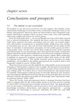
Grab-type mechanical dredges are used commonly in lake restoration (Figure 20.1). Figure 20.1A
shows a clamshell bucket dredge in operation. Figure 20.1B shows a typical Sauerman grab bucket
set-up. A limitation of all grab bucket dredges is that they must discharge in the immediate vicinity
of the sediment removal area or into barges or trucks for transportation to the disposal area. Their
normal reach is no more than 30 to 40 m. Another disadvantage is the rough, uneven bottom contours
they create. Production rates are relatively slow due to the time-consuming bucket swing, drop,
close, retrieve, lift, and dump operating cycle. Grab dredges commonly create very turbid water
conditions due to bucket drag on the bottom as it pulls free from the sediment, dragging an open
bucket through the water column, bucket leakage once it clears the water surface, and the occasional
intentional overflow of receiving barges to increase their solids content. Another disadvantage is
that many lake sediments are highly flocculent, reducing the pickup efficiency of a grab bucket.
Grab-bucket dredges have at least two advantages over the other dredge types: they can be
transported with ease from one location to another and they can work in relatively confined areas.
Thus, their chief use in lake restoration and management is shoreline modification, particularly
around docks and marinas. They are readily operated around stumps and trash frequently found in
these areas. A grab bucket operates most efficiently in near-shore areas that contain soft to stiff
mud. Depth is no impedance, but efficiency drops rapidly with depth, because of the time consuming
operating cycle.
Silt curtains reduce some of the turbidity-associated problems mentioned above. A silt curtain
is a continuous polyethylene sheet (skirt) buoyed at the surface and weighted at the bottom so it
hangs perpendicular to the water surface. It may be used to encircle an open water dredging

operation or to isolate a length of shoreline (Figure 20.1). The purpose of the silt curtain is to
isolate turbidity within the immediate dredging area, protecting clean surface water areas down-
stream. Silt curtains, while effective in controlling surface turbidity, are open at the bottom and
permit the escape of turbid water near the sediment–water interface.
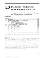
Another means of minimizing turbidity from grab bucket dredging is to use a covered, watertight
unit (Figure 20.2). Watertight buckets range in sizes from 2 to 20 m
3
. Manufacturers claim turbidity
reductions from 30% to 70% compared to open buckets of comparable size. The dredging process
with watertight buckets is cleaner than with conventional buckets, but production is still relatively
inefficient compared to hydraulic dredges.
20.5.2 HYDRAULIC DREDGES
There are many variations of hydraulic dredges, including the suction dredge, the hopper, the
dustpan, and the cutterhead suction dredge. Hopper dredges are impractical for dredging small
inland lakes. Cutterless suction dredges have not been used extensively. Attempts to use one at
Lilly Lake, WI, in 1978 were abandoned when it was discovered that the partially decomposed
plant material in the sediment prevented it from “flowing” to the suction head (Dunst, 1982). A
cutterhead suction dredge subsequently was employed.
Dustpan dredges are not commonly used in lake restoration, although a “dustpan-like” dredge
was used to remove flocculent sediment from Green Lake, Washington in 1961 and 1962 (Pierce,
Copyright © 2005 by Taylor & Francis
1970). The device consisted of a 15.25 m suction manifold with slot openings. The total size of
the inlet ports was designed to produce inlet velocities of at least 300 cm/s. As sediment consistency
increased with depth, some of the inlet ports were sealed to increase flow velocity in the open
ones. The dustpan-like suction head was barge mounted and designed to swing in a full 180° arc
and discharge into a 50.8 cm diameter pipeline. The discharge distance was about 792 m. This
dredge successfully removed 917,500 m
3
of sediment. Björk (1974) indicated that the dredge head
used at Lake Trummen, Sweden had a specially designed “nozzle.” The positive experience at

Green Lake and at Lake Trummen indicates that dustpan types and other variations of conventional
hydraulic suction heads should receive additional consideration for dredging highly flocculent fresh
water lake sediments.
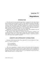
FIGURE 20.1 (A) Silt-curtain encirclement of an open-water grab dredge operation. (B) Shoreline isolation
of a bucket dredge operation, using a silt curtain. (Cooke et al., 1993. With permission.)
A
Dredge
bucket
Buoys
Shoreline
Barge
Silt
curtain
Silt
curtain
Sediment
surface
B
Sediment surface
Buoys
Dredge
bucket
Copyright © 2005 by Taylor & Francis
Inland lake sediment removal is most commonly accomplished with a cutterhead hydraulic
pipeline dredge. Small, portable, cutterhead hydraulic dredges are the dominant equipment used
for inland lake dredging. The primary components of any cutterhead dredge system include the
hull, cutter head, ladder, pump, power unit, and a pipeline to distribute dredged material (Figure
20.3).
The hull is made of steel and constructed to withstand the constant vibration created by the
cutterhead. The hull is the working platform that houses the main power plant, pump, lever room,

and the assemblage of winches, wires, “A” frames, etc., that comprise the dredge.
At the bow is a steel boom or ladder with a cutter mounted at its distal end. Ladder length
determines the practical dredge depth limitations. The ladder also supports the suction pipe and
the cutter drive motor and shaft. In some cases, there may be a submersible auxiliary suction pump
mounted on the ladder. The ladder is raised and lowered by suspension cables attached at the outer
end and to a hull-mounted winch.

The cutter or cutterhead typically consists of three to six smooth or toothed conical blades that
rotate at 10 to 30 rpm to loosen compacted sediment (Bray, 1979). Cutterheads may be open nose,
closed nose, straight vane, ribbon screw shape, or auger-like. Most cutters have been designed
specifically to loosen sand, silt, clay, or even rock material. Few, if any conventional hydraulic
cutterheads have been designed to remove soft, flocculent lake sediment, so most of them are less
efficient than they could be for lake dredging.
Spuds, vertically mounted pipes ranging from 25.4 cm to 127 cm in diameter, depending on
the dredge size, are located at the stern of the hull on both sides (Figure 20.4). They are used to
“walk” the dredge forward by alternately raising and lowering them into the sediment.
Operationally, sediment loosened by the cutter moves to the pickup head by suction from the
dredge pump, usually a centrifugal type. The sediment slurry is then discharged by pipeline to a
remote disposal area. Cutterhead dredges are described by the diameters of their discharge pipes.
Hydraulic dredges used for inland lake work usually range in size from 15 to 35 cm, although the
one used at Vancouver Lake, Washington was 66 cm (Raymond and Cooper, 1984). Figure 20.4
shows how the cutterhead is moved from side to side, and how pulling alternately on port and
starboard swing wires creates the cut path. A major advantage of hydraulic cutter suction dredges
over bucket types is that they are not confined in operation by the limitation of cable reaches.
Another advantage is their continuous operating cycle. This cycle permits hydraulic dredges to
FIGURE 20.2 Open and closed positions of the watertight bucket. (Redrawn from Barnard, W.D. 1978.
Prediction and Control of Dredged Material Dispersion Around Dredging and Open-water Pipeline Disposal
Operations. Tech. Rept. DS-78-13. U.S. Army Corps Engineers, Vicksburg, MS.)
Shell
Rod

Rod
Cover
Cover
Rubber
packing
Open position Closed position
Shell
Copyright © 2005 by Taylor & Francis
produce large volumes of dredged material. This advantage, however, is not without its downside.
Most hydraulic dredge slurries contain only 10% to 20% solids and 80% to 90% water. This means
that relatively large disposal areas, with adequate residence times, are needed to precipitate solids
from the dredge slurry. Also, it means that the large pumping capacity of hydraulic dredges might
produce unplanned lake drawdowns, unless disposal-area overflow water is returned to the lake.
The amount of sediment supplied to the suction head is controlled by cutter rotation rate,
thickness of the cut, and the swing rate (Barnard, 1978). Improper combination of any of these
FIGURE 20.3 Configuration of a typical cutterhead dredge. (From Barnard, W.D. 1978. Prediction and
Control of Dredged Material Dispersion Around Dredging and Open-water Pipeline Disposal Operations.
Tech. Rept. DS-78-13. U.S. Army Corps Engineers, Vicksburg, MS.)
FIGURE 20.4 Spud-stabbing method for forward movement, and resultant pattern of the cut. (From Barnard,
W.D. 1978. Prediction and Control of Dredged Material Dispersion Around Dredging and Open-water Pipeline
Disposal Operations. Tech. Rept. DS-78-13. U.S. Army Corps Engineers, Vicksburg, MS.)
Cutter
Sediment
Shaft
A frame
Cutter
motor
Ladder
Suction
Hoist

Lever room
Gantry
Engine house
Spud well
Spud
Floating
line
Main pump
H frame
Hull
Winch
Dredge
Advance
Cut “A”
Spud (up)
Spud
(down)
A
B
C
D
Ladder
B
D
AC
Front
Windrow
Starboard
swing wire
Port

swing wire
Cutter
Copyright © 2005 by Taylor & Francis
might result in excessive turbidity. Therefore, not only the configuration of the dredge equipment,
but the skill of the operator is important to minimizing turbidity. New computer technology on
special purpose dredges has reduced this problem considerably.

20.5.3 SPECIAL-PURPOSE DREDGES
Portable cutterhead dredges are essentially miniatures of large coastal waterway dredges. The
cutterheads of coastal dredges were designed for cutting sand, clay, and silt; they were not intended
for use in fine, flocculent, organic lake sediments (frequently 40% to 60% organics). Consequently,
soft lake sediments have challenged the dredging industry that responded with several dredging
innovations. Among them is the cutter head used on Mud Cat
®
dredges. These dredges utilize a
horizontal auger to dislodge and move sediment to the center of a 2.4 m wide, shielded, dredge
head where it is sucked up by the pump and transported through a 20.3 cm discharge pipeline.
Mention of the Mud Cat dredge is to illustrate their auger type cutter head and the mobility of
small dredges (Figure 20.5). There are several others that are just as portable (see Clark, 1983).
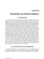
Note in Figure 20.5 the mud shield, which can be raised or lowered over the auger head to
minimize sediment resuspension. Nawrocki (1974) reported that turbidity plumes due to dredging
with a Mud Cat machine were confined to an area no more than 6 m from the dredge, though
operating conditions were not clearly defined. Suspended solids in the area of increased turbidity
ranged from 39 to 1,260 mg/L. Those near the bottom averaged approximately 100 mg/L. More turbidity
is created by forward motion of the dredge than by backward motion. This appears to be caused by
raising the mud shield while moving forward, but lowering it when moving backward. Mallory and
Nawrocki (1974) indicated that the Mud Cat dredge should be capable of producing slurry con-
FIGURE 20.5 The Mud Cat
®
dredge features a unique auger-type cutterhead. The size of the dredge makes

it extremely portable. (Photo courtesy of Ellicott, Division of Baltimore Dredges, LLC, Baltimore, MD.)
Copyright © 2005 by Taylor & Francis
taining 30% to 40% solids. This represents nearly a doubling of the solids content commonly
produced by conventional cutterhead dredges.
The Mud Cat guidance system is well suited to work on small water bodies. The dredge operates
on a cable anchored at both shorelines. The guidance system permits uniform dredging of the
bottom, with few missed strips. Mud Cat dredges have been used successfully at Collins Park and
several other small lakes in New York State. The portability, guidance system, reduced turbidity,
and increased solids content resulting from use of these dredges makes them ideally suited to small
lake restoration projects. New and improved guidance and operating systems on Mud Cat
®
dredges
have been instrumental in successful dredging of lakes in Europe (see case histories in this chapter).
Clark (1983) reported on a survey of portable hydraulic dredges available for use in the U.S.
The survey identified 46 models of portable equipment available from several different manufac-
turers. No attempt was made to critically analyze the features of one dredge relative to another,
but tables are presented that describe the general dredge specifications, the pump characteristics,
suction and discharge diameters, cutter type, and working capacity. The information should be
useful to engineers for selecting dredges, since it includes dredging depth ranges from 3 to 18 m,
production rate ranges from 15 to 1375 m
3
/h, and a wide variety of cutterhead types.
Equipment that removes water from hydraulically dredged material by centrifugal force exists,
but we are not aware of any published evaluations. While this technique would reduce pond holding
times for sediment settling, the high volume of water (typically 80% to 85%) in dredged material
would still need to be managed.
20.5.4 PNEUMATIC DREDGES
Pneumatic (air-driven) dredge systems might have several advantages over conventional dredge
systems relative to removal of fine grain lake sediment (Cooke et al., 1993). All of the pneuma
systems (Oozer

®
, Cleanup
®
, Pneuma
®
) are Japanese. To our knowledge, the only use of one of
these systems was the Ooozer-like (Figure 20.6) pneuma pump used at Gibraltar Lake, CA in 1981
(Spencer Engineering, 1981) to remove mercury-contaminated sediments.
After major modification of the valving material in the pump body, the pneumatic system
performed satisfactorily (Spencer Engineering, 1981). Goldman et al. (1981) confirmed these
findings and reported there were no elevated mercury levels in the water column at any station or
at any depth during dredging. The dredging was so clean that no bathing beach areas in the 110.8
ha lake were forced to close during any phase of the dredging. Despite these positive findings,
pneumatic dredging systems have not been used widely in the United States and, therefore, will
not be discussed further in this text.
20.6 SUITABLE LAKE CONDITIONS
Peterson (1981, 1982a) described some sediment problems to consider when assessing dredging
feasibility. Lake size, except for total cost, is not a dredging constraint. Peterson’s (1979) exami-
nation of 64 lake-dredging projects showed that size ranged from less than 2 to over 1,050 ha, and
that sediment volume removed ranged from a few hundred to over 7 million cubic meters.
One factor that might limit dredging of a large inland lake is the requirement for a commen-
surately large disposal area. Restoration most frequently is sought for lakes in high use areas, where
sediment disposal space is scarce, but also where the greatest user benefits will be derived (JACA,
1980). Therefore, it is important that disposal alternatives be explored for these situations.
Various productive uses of dredged material have been examined (Lunz et al., 1978; Spaine et
al., 1978; Walsh and Malkasian, 1978). At Nutting Lake, MA, 153 × 103 m
3
of sediment was
sold as soil conditioner at $1.40/m
3

. This reduced the total dredging cost by $215,000 and per
unit dredging cost to about $1/m
3
(Worth, 1981). However, the final Nutting Lake report refutes
this information saying that no substantial income was realized from the sale of dredged material
Copyright © 2005 by Taylor & Francis
(Baystate Environmental Consultants, 1987). This was attributed to excavation difficulties fostered
by the slow drying of material in the disposal basins. But, the containment area subsequently was
sold for $450,000, nearly recovering the invested project costs. In Japan, sediment disposal areas
are commonly sold for industrial development or converted to parks (Matsubara, 1979).
To be cost effective, a sediment removal project should have reasonable assurance of longevity.
An estimate of sedimentation rates helps determine the infilling rate and, thus the duration of
sediment removal effectiveness. Although dredging is expensive per unit of dredged material, where
costs are amortized over the life expectancy of the project they may look much more reasonable.
All other conditions being similar, lakes with relatively small watershed-to-surface ratios (nominally
10:1) will have lower sedimentation rates than those with large watersheds. Thus, a large lake with
a small watershed should benefit more from dredging than will the reverse situation.
Depth, size, disposal area, watershed area, and sedimentation rate described above are all
physical features. What about the influence of sediment chemistry on lake biota? Current infor-
mation demonstrates that lakes with highly enriched surface sediments relative to underlying
sediment (see Lake Trummen case history) might benefit from shallow dredging (Andersson et
al., 1975; Bengtsson et al., 1975). Lake Trummen, Sweden, showed marked changes in water
chemistry and biota when 40 cm of rich surface sediments were removed (Björk, 1978). Similar
changes were observed in Steinmetz Lake, NY, when 25 cm of organic sediments were removed
and replaced by the same amount of clean sand (Snow et al., 1980). In both cases, extensive
sediment surveys before dredging revealed that surface sediment was disproportionately rich in P
and N relative to the deeper sediment. In lakes, open water sediment is usually more important in
sediment surveys than littoral zones, since sediment is transported toward the deeper zones of lakes.
Surface inflow areas also need to be considered. Littoral zones tend to be cleaned by wave action
and, in the temperate zone, by spring ice scouring. Reservoirs accumulate sediment quickly at their

inflows due to their extensive watersheds. Sediment surveys should, at the minimum, determine the
area of sediment to be removed and the depth (see the next section). Horizontal sediment characteristics
normally are more uniform than vertical sediment profiles. Sediment depth may vary considerably,
depending on the basin configuration at the time of the lake formation or the transport of sediment
to the lake via stream inlets. Vertical variation in the survey is important to note. Sediment profiles
can be developed with the assistance of a Livingston piston corer. It is important to note sediment
color and texture differences with depth and to chemically characterize (P and N) surface (0 to
approximately 10 cm) sediment relative to deeper sediment if nutrient control is the intent (Peterson,
FIGURE 20.6 Schematic diagram of Oozer
®
dredge system. (Cooke et al., 1993. With permission.)
Direction
of swing
Filling phase
Hydrostatic
pressure
Hydrostatic
pressure
Air pressure
From
air pump
To discharge
pipe
Suction head
Sediment Sediment
Hydrostatic
pressure
Hydrostatic
pressure
Negative

pressure
To vacuum
pump
Sediment level
indicators
Empty Full
Discharge phase
Copyright © 2005 by Taylor & Francis
1981). Beyond this it is quite useful to know sediment particle size, settling rate, sediment volume,
etc., to properly select a dredge for the job and design an adequate disposal area.
Several variables determine the suitability of a lake for dredging, but generally the most suitable
lakes have shallow depths, low sedimentation rates, organically rich sediments, relatively small
(10:1) watershed-to-surface ratios, long hydraulic residence times, and the potential for extensive
use following dredging.
20.7 DREDGE SELECTION AND DISPOSAL AREA DESIGN
This section draws heavily from the work of Pierce (1970). Implementation of lake dredging requires
several decisions. The most important ones are what dredging equipment to use and what factors
to consider in the disposal area design. Equipment selection depends on several variables, including
availability, project time constraints, slurry transport distances, discharge head, and the physical
and chemical characteristics of the dredged material.
The primary factor controlling the disposal area design is the amount of dredged material that
must be contained. A second factor is the need to meet the discharge permit suspended solids
requirements. Therefore, sediment grain size, specific gravity, plasticity, and settling characteristics
of the dredged material must be considered when designing the disposal area.
To illustrate these considerations an example is offered. A feasibility study conducted on
hypothetical Dead Lake, located in a rural area of the glaciated upper mid-western U.S. reveals
these characteristics:
• Lake area = 120 ha
• Maximum depth = 5.5 m
• Average depth = 2.0 m

• Normal water level = 245 m above sea level
• Sediment water content = 30% to 60%
Since total project cost is usually based on a measure of actual material removed, it is necessary
to estimate the amount and type of sediment contained in the basin. The usual procedure is to
collect hydrographic data suitable to developing a lake-bottom map that describes the configuration
of the original basin. The accuracy of this map depends on the sampling interval and the original
basin relief. Even relatively shallow glacial lakes may have deep holes, reinforcing the need for
sediment depth mapping.
Sediment sampling frequency to determine volume varies depending on basin configuration
and desired survey accuracy. Preliminary sampling stations should be broadly spaced to provide a
rough estimate of the solid bottom relief of the lake. This helps define and limit the required number
of stations for final mapping. Pierce (1970) suggested that small to medium sized (< 40.5 ha) sediment
removal projects should be mapped routinely by laying out sampling locations in a 15.25 m grid
pattern. Pattern layout can be done by survey or using GPS units. He also suggested that, for lakes
with surface areas > 40.5 ha, the sample station grid size could be increased to 30.5 m without
significant loss of accuracy. He noted further that there will be far less variance horizontally than
there will be vertically in lake sediment quality. Individual lake characteristics ultimately dictate
the required station frequency.
A common procedure for obtaining the necessary data is to make sediment depth/lake hard
bottom measurements at stations prescribed by the chosen grid size and relating the measurements
to known elevation datum points on shore (topographic map, U.S. Geological Survey bench mark,
etc.). The measurements can then be converted to elevations, thereby permitting the development
of hydrographic maps and calculation of sediment volume.
A simple means of obtaining the required data is to measure, at each station, the water depth
to the sediment–water interface and the distance (depth) to which a probe can be pushed into the
Copyright © 2005 by Taylor & Francis
lake sediment before contacting hard bottom. Both measurements can be made at the same time
by using a graduated probing (“sounding”) rod. Lake sediment probes usually are steel rods
measuring 0.95 cm to 1.6 cm in diameter. If the rods are forced they can be bent and accuracy is
reduced. The investigator needs to develop “a feel” for the degree of resistance that determines

hard lake bottom. Sediment depth is determined by calculating the difference between the rod
interval reading at “hard bottom” and the reading at the sediment–water interface. Distinction of
the sediment–water interface may be difficult in lakes with flocculent, highly organic sediments.
In these cases, it is advisable to use a lightweight disc or foot at the tip of the probing rod to
establish water depth to the sediment surface. Alternatives to this are the use of a graduated line
and Secchi disk, or an electronic depth sounder, some of which are extremely accurate.
Depth determination is easiest during calm periods on open waters and pontoon boats are great
platforms for doing this work. In cold climates the work can be accomplished even more easily by
making the measurements through holes drilled in the ice. Winter lake mapping makes it much
easier to locate your position accurately, particularly when using GPS. Pierce (1970) indicated that
a properly equipped crew working efficiently should be able to collect water and sediment data in
this manner over 4 to 8 ha of lake surface per day. Efficiency is enhanced if data are collected
during early winter; before ice has thickened to more than 15 or 20 cm. Sediment depth measurement
is critical. Miscalculations in the sediment volume leads to errors in projecting cost estimates and
to selecting proper dredging equipment, so accuracy should be stressed.
Sediment mapping of Dead Lake indicated deposits of highly organic silt material (muck).
Water content of surface sediment averaged about 60%, while that at mid-depth and beyond ranged
from 30% to 40%. Mapping data showed that sediment thickness was nearly 3.6 m at the south
end, near the inlet, and that it decreased to about 1.8 m on the north end. These sediment conditions
are well suited to the use of a hydraulic cutterhead dredge. Three sediment disposal areas were
located around the lake. The desire to minimize pumping distances made it convenient to divide
the lake surface area into three pieces; each one identified with the nearest disposal area. Figure
20.7 shows how the lake might be divided to best utilize the available upland disposal areas.
The feasibility study shows that sedimentation rates in the lake have been reduced significantly
over the past 15 years as a result of shifts from row crop to small grain and hay crop farming in
the watershed. The accumulated sediment is not contaminated, and recent accumulations result
mostly from autochthonous organic material decomposition. Therefore, it appears that deepening
at least 15% of the lake to about 6.0 m, while leaving a fish spawning and wildlife area intact, will
have a positive effect toward restoring the fishery and other beneficial uses. The study indicated
further that water depth 60 m from shore should be a minimum of 2.5 m, and that the bottom

should then slope at a 5% grade to a depth of 3.5 m. Reconfiguring the lake in this manner will
provide adequate water volume and depth to maintain adequate dissolved oxygen (DO) levels to
avoid fish winterkills (Toubier and Westmacott, 1976).
The maximum depth calculations based on these recommendations indicate that approximately
1,530,000 m
3
of sediment needs to be removed. It is desirable to complete the project as rapidly
as possible, to minimize lake use disruption, so project duration is targeted for 2 years (mid-April
through mid-November: ice-free months, over two consecutive seasons).
20.7.1 DREDGE SELECTION
Proper selection and use of hydraulic dredging equipment will implement feasibility recommen-
dations. The remainder of this section presents a series of considerations for selecting a cutterhead
dredge (Pierce, 1970).
20.7.1.1 Plan to Optimize the Available Disposal Area
Long pumping distances to disposal areas should be minimized, since energy requirements increase
with pumping distances. Disposal area No. 1 is the closest, at 750 m, when pumping from lake
Copyright © 2005 by Taylor & Francis
area No. 1 (Figure 20.7). Disposal area No. 2 is 800 m and disposal area No. 3 is 1,900 m, when
pumping from the respective lake areas. It was calculated that areas 1, 2, and 3 will hold 574,000,
413,000, and 918,000 m
3
of dredged material, respectively. Therefore, areas 1 and 2 would receive
574,000 and 413,000 m
3
, respectively, with area 3 receiving the remainder of the dredged material
(543,000 m
3
), to optimize disposal efficiency by minimizing pipeline length.
20.7.1.2 Analyze the Production Capacity of Available Dredging Equipment
It is necessary to analyze the production of various sized dredges to determine which equipment

might complete the job within the planned 2-year period. A survey of equipment reveals that 20-
cm, 25-cm, and 30-cm dredges are available, so production analysis is limited to these sizes.
Dredge pump production rates usually are listed as ranges since dredging conditions, and thus
production rates, vary considerably. Production ranges for the available dredges (20, 25, and 30
cm) are taken from Figure 20.8 to illustrate the method. Similar dredge capacity charts are available
from various dredge pump manufacturers. Charts for the specific equipment in question should be
used whenever they are available. Figure 20.7 and the feasibility study for Dead Lake showed that
the greatest sediment volume is located near the center of the lake and that transport from this area
to the disposal cells will require pipeline transport distances in excess of 600 m. Based on that
information, the following dredge pump production range analysis was developed, using the min-
imum, a medium, and the maximum pipeline lengths:
300-m length of discharge pipeline:
20-cm pump = 50 to 110 m
3
/h, average 80 m
3
/h
25-cm pump = 80 to 190 m
3
/h, average 135 m
3
/h
30-cm pump = 310 to 420 m
3
/h, average 365 m
3
/h
600-m length of discharge pipeline:
FIGURE 20.7 Dead Lake (hypothetical), showing the planned dredging areas, pipeline distances to disposal
areas, and the wildlife area that will remain undredged (not to scale). (Cooke et al., 1993.With permission.)

150 m
200 m
600 m
1150 m
750 m
600 m
1
2
3
Disposal area
No. 1
elev. = 247.7 m
Disposal area
No. 3
elev. = 251 m
Disposal area
No. 2
elev. = 247.7 m
Normal lake elev. = 245 m
Wildlife preserve
Copyright © 2005 by Taylor & Francis
20-cm pump = beyond effective discharge length; booster pump required
25-cm pump = 60 to 120 m
3
/h, average 90 m
3
/h
30-cm pump = 220 to 290 m
3
/h, average 255 m

3
/h
800-m length of discharge pipeline:
20-cm pump = beyond effective discharge length; booster pump required
25-cm pump = 50 to 80 m
3
/h, average 65 m
3
/h
30-cm pump = 190 to 250 m
3
/h, average 220 m
3
/h
The analysis reveals that use of the 25 cm system for distances of 600 to 800 m is marginally
efficient, based primarily on the dredge pump characteristics and its power (kilowatts). As pipeline
length increases pipeline friction increases and solids transport efficiency decreases. A pipeline
discharge velocity of 3 to 4 m/s must be maintained to transport solids. Thus, discharge pipeline
length must be limited to that which permits the velocity to be maintained at 3 to 4 m/s. Longer
FIGURE 20.8 Representative production characteristics for various sizes of dredge systems. (Modified from
Pierce, N.D. 1970. Inland Lake Dredging Evaluation. Tech. Bull. 46. Wisconsin Dept. Nat. Res., Madison.)
Solids pumped (m
3
hr
−1
)
800
600
400
200

500
400
300
200
100
0
0
200
300
400
500
600
800
1000
200
300
30 cm dredge 35 cm dredge
20 cm dredge
400
500
600
800
1000
100
200
300
400
600
800
100

200
300
400
600
800
25 cm dredge
Length of discharge pipeline (m)
Copyright © 2005 by Taylor & Francis
pipes can be used with booster pumps. The analysis indicated that disposal in cell No. 3 from lake
area No. 3, even with the largest system available (30 cm), would require a booster pump.
20.7.1.3 Compute Dredging Days Required to Complete the Job
Approximately 1,530,000 m
3
of sediment must be removed from Dead Lake. For efficiency, a
hydraulic dredge normally operates 24 h/d unless noise is a problem. Noise could be a concern on
urban or small lakes.
There is always some down time for maintenance and pipeline relocation, so for this example
we will assume a 24 h/d operation schedule with a normal productive dredge time of approximately
20 h/d, 6 d/week.
Previously, it was observed from the above production analysis that the 20 cm dredge would
not operate efficiently without a booster pump at discharge distances exceeding 600 m. Since most
of the pumping will require discharge at 600 m and beyond, the 20 cm pump should not be
considered. Using the average (rounded down for illustrative convenience) discharge rates of the
25 cm and 30 cm systems for 600 m and 800 m pipeline lengths (Figure 20.8 or the discharge
pipeline summary above) the number of days required to complete the Dead Lake dredging project
can be calculated.
25 cm pump system:
30 cm pump system:
Dead Lake is located in the northern U.S. so it is frozen over from approximately mid-November
until mid-April. This reduces annual open water workdays to about 185. If the 25 cm pump system

is used, completion time would exceed 5 years (1,020 ÷ 185 = 5.5 year). If the project is to be
completed within the 2 year target time (two open water seasons), the 30 cm dredge is required
(333 ÷ 185 = 1.8 year). Disposal in area No. 3 requires use of an appropriately placed booster
pump, since the pipeline length to that area exceeds the efficient pumping distance (approximately
1000 m) of the 30 cm pump system.
20.7.1.4 Determine the Required Head Discharge Characteristics of the
Main Pump When Pumping Material with the Specific Gravity of
Lake Sediment (Approximately 1.20)
The required head-discharge characteristics of a pump depend on the discharge pipe length, i.e.,
the longer the pipeline, the higher the total head required. Pump head discharge characteristics
must be analyzed for both minimum and maximum discharge distances. In the case of Dead Lake,
the minimum is about 300 m (150 m from shore to disposal area plus 150 m off-shore in the lake)
90 65
2
77
1 530 000
33
33
mh mh
5m h 75m h
//
./ /
,,
+
=≅
m
mh hd
1020 d
3
3

75 20(/)(/)
=
255 220
2
237 5 230
1 530
33
33
mh mh
mh mh
//
./ /
,
+
=≅
,,
(/)(/)
000
230 20
333
3
3
m
mh hd
d=
Copyright © 2005 by Taylor & Francis
since dredging to the shoreline is seldom done when pumping from lake area 1 to disposal area 1,
and the maximum is about 1,900 m when pumping from lake area 3 to disposal area 3.
The sum of the total suction lift and total discharge head is the total dynamic head against
which a pump works (Pierce, 1970). Heads commonly are computed from basic hydraulic formulae,

corrected for specific gravity of the pumped material. Suction lift incorporates suction elevation
head, suction velocity head, and friction head in the suction pipe. The total discharge head is
calculated by summing the pump velocity head, the discharge elevation head, and the friction head
in the pipeline. Minor head losses usually are not considered.
20.7.1.4.1 Suction Head
Since the weight of dredged material (specific gravity of lake sediment is approximately 1.20) is
greater than water, the surface of a column of water equal to the depth of Dead Lake would always
have a greater elevation than the surface of an equal sized (diameter) column of dredged material
of the same weight. The resultant difference in column heights is the suction elevation head. The
suction elevation head always refers to the horizontal center line of the main pump and is computed as
(20.2)
where: h
ss
= the suction elevation head (meters of fresh water), S
1
= specific gravity of lake water
(1.0), S
2
= specific gravity of material being pumped (1.2), A = distance from the bottom of the
cut to the water surface (m), and B = distance from the pump center to the bottom of the cut (m).
Assuming that the dredge pump is mounted on the hull at lake level and that maximum dredged
depth is 8.5 m, the static suction head is
The minus sign indicates that a suction head exists. This number must be added positively to other
heads computed for the suction system.
The suction velocity head is the energy required to start the movement of dredge material into
the suction pipe. It can be computed as
(20.3)
where: h
sv
= velocity head (meters of fresh water), S

2
= specific gravity of the material being
pumped, Vs = velocity of the mixture in the suction pipe (m/s), and g = acceleration rate of gravity
(m/s
2
).
The acceleration rate of gravity is 9.82 m/s
2
. Normal suction pipe velocity should be maintained
at 3.0 to 4.0 m/s to assure that solids are carried into the pump. If we assume an upper midrange
suction pipe velocity of 3.6 m/s, the velocity head in the suction pipe will be
hSASB
ss
=−
12
h
h
ss
ss
=−
=−
10085 12085
17
.(.) .(.)
.m
h
Vs
sv
g
= S

2
2
2
h
h
sv
sv
=
=
(. )
(.)
(. )
.
120
36
2982
08
2
m
Copyright © 2005 by Taylor & Francis
Friction head losses caused by aqueous flow characteristics in pipes create the major portion
of the head that a dredge pump must overcome. Pipeline friction loss is influenced by several
variables. Among them are the type and diameter of pipe, flow velocity in the pipe, pipeline length
and configuration, and the percentage and type of solids in the pumped mixture. Since friction losses
are magnified as the diameter of the suction pipe decreases, many small dredges utilize suction
pipes one size (usually 5 cm increments) larger than the discharge pipe. For example, a 30-cm
dredge (size of discharge) might have a 35 cm suction line. Velocity in the discharge pipe (30 cm)
will be greater than that in the suction pipe (35 cm), since the volume entering the larger suction
pipe must be squeezed through the smaller diameter discharge pipe. The velocity in the discharge
pipe varies as the ratio of the square of the diameter of the larger pipe divided by the square of

the diameter of the smaller one [(35)
2
÷ (30)
2
= 1.36]. Therefore, the 3.6 m/s velocity in the suction
will be increased to approximately 4.9 m/s in the discharge. All influences affecting pipeline friction
losses (suction friction head) must be considered and applied to an acceptable equation for formu-
lating friction losses. Suction friction head is the energy required to overcome friction losses in the
pump suction line (Pierce, 1970). The suction friction head can be computed from the Darcy–Weis-
bach formula:
(20.4)
where: h
sƒ
= friction head (meters of fresh water), ƒ = the friction factor, P = solids in dredge slurry
(% by volume), L = equivalent length of suction pipe (m), Vs = velocity of the mixture in the
suction pipe (m/s), g = acceleration rate of gravity (m/s
2
), and D = inside diameter of the suction
pipe (m).
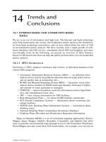
The friction factor ( ƒ ) is a dimensionless number that is a function of the Reynolds number
and the relative roughness (absolute roughness ÷ diameter of pipe in m) of different types of pipe.
The functions have been obtained experimentally for clear water and expressed graphically (Figure
20.9) by Moody (1944). Use of ƒ as described by the Moody diagram for computing dredged
material pipeline transport necessarily becomes an approximation at best, since solids in the slurry
will affect the number. Despite this apparent problem, Moody ( ƒ) values are commonly used to
estimate various hydraulic, pipeline dredging figures. The Reynolds number can be calculated from
the formula
(20.5)
where: V = velocity in the pipeline (m/s), D = inside diameter of the pipeline (m), and v =
temperature-corrected kinematic viscosity of water (m

2
/s × 10
−6
) (see Table 20.1).
As stated above, the velocity of suction pipeline slurries commonly ranges from 3.0 to 4.0 m/s
or greater to maintain the suspension of solids (turbulent flow). If we use the previous assumed
slurry velocity of 3.6 m/s and a kinematic viscosity of water at 20°C (1.0 × 10
6
m
2
/s) and apply
these figures to a 35 cm (0.35 m) suction pipe, the following Reynolds number can be calculated
from Equation 20.5
h
PLV
gD
sf
s
=
+−
⎡
⎣
⎢
⎤
⎦
⎥
f
110
100 2
2

()
R
VD
v
=
R
R
=
×
=×
−
36 035
10 10
13 10
6
6
.(.)
.
.
Copyright © 2005 by Taylor & Francis
If we assume a pipe roughness of 8.7 × 10
−5
m, the relative roughness will be
(20.6)
where: rr = relative roughness, e = absolute roughness (m), D = inside diameter of pipe (m).
Then
Applying relative roughness and the Reynolds number to the Moody diagram (Figure 20.9), the
resultant friction factor is 0.015 for these conditions. Note that the intersection of these two variables
falls within the transition zone between laminar flow and complete turbulence in rough pipes.
Friction-head losses in suction pipes vary with configuration, valving, suspended solids concen-

tration, and cutterhead types. Cutterhead losses are highly variable and losses associated with fine
grain dredge material are not well defined. (Note the comment above concerning the use of ƒ values.)
Correction factors for these variables are not readily available in tabular form. Therefore,
engineering best judgment based on a combination of practical experience and laboratory tests
frequently is applied to actual suction pipe lengths to calculate “the equivalent length of suction
FIGURE 20.9 Moody diagram showing friction factors for pipe flows. (Redrawn from Moody, L.F. 1944.
Trans. ASME 66: 51–61. With permission.)
10
3
2468 246810
4
Complete turbulence, rough pipes
Laminar
flow
Critical
zone
Transition
zone
Surface type
⑀, m
Riveted steel
Concrete
9.14 × 10
−4
− 9.14 × 10
−3

3.05 × 10
−4
− 3.05 × 10

−3

1.83 × 10
−4
− 9.14 × 10
−4

2.59 × 10
−4

1.52 × 10
−4

1.22 × 10
−4

4.57 × 10
−5

1.52 × 10
−6
Plain cast iron
Galvanized iron
Wood stave
Asphalted cast iron
Commercial steel
or wrought iron
Drawn tubing
0.100
0.090

0.080
0.070
0.060
0.050
0.040
0.030
0.025
0.020
0.015
0.010
0.009
0.008
22424466688810
5
10
6
10
7
10
8
0.05
0.04
0.03
0.02
0.015
0.010
0.008
0.006
0.004
0.002

0.0008
0.001
0.0006
0.0004
0.0002
0.0001
0.00005
0.00001
⑀/D = 0.000001
⑀/D = 0.000005
Reynolds number =
Friction factor ∫ =
H
L
2gD
LV
2
Relative rou
g
hness (⑀/D)
Laminar
flow
Smooth pipes
Absolute Roughness of New, Clean,
Pipe Walls
VD
ν
rr
e
D

=
rr
rr
=
×
=×
−
−
87 10
035
25 10
5
4
.
.
.
Copyright © 2005 by Taylor & Francis
pipe.” In effect, the equivalent length is a correction for suction pipe head loss. The suction pipe
“correction factor” commonly is within the range of 1.3 to 1.7 (Hayes, 1980). To dredge to a depth
of 8.5 m (maximum lake depth after dredging), the dredge ladder (suction pipe length) will need
to be approximately 15 m long. Applying a suction-pipe-equivalency correction factor of 1.7, the
equivalent suction pipe length is 25.5 m (15 × 1.7 = 25.5). Substituting the required figures (assume
20% solids) into Equation 20.4 determines the suction friction head
The total suction head (H
s
) on the dredge pump is the sum of the suction elevation head (-1.7,
added positively), the velocity head (0.8) and the friction head (0.8)
20.7.1.4.2 Discharge Head
Discharge elevation head is represented by the difference in elevation (vertical distance) between
the pump centerline and the end of the discharge pipe, corrected for the specific gravity of the

TABLE 20.1
Selected Physical Properties of Water at Various Temperatures
Temp erature
T (°C)
Density
p (g/cm
3
)
Viscosity
μ (g/cm/s ×10
2
)
Kinematic Viscosity
v (cm
2
/s × 10
2
)
a
0 0.9999 1.787 1.787
5 1.0000 1.514 1.514
10 0.9997 1.304 1.304
15 0.9991 1.137 1.138
20 0.9982 1.002 1.004
25 0.9971 0.891 0.894
30 0.9957 0.798 0.802
35 0.9941 0.720 0.725
40 0.9923 0.654 0.659
50 0.9881 0.548 0.554
60 0.9832 0.467 0.475

70 0.9778 0.405 0.414
80 0.9718 0.355 0.366
90 0.9653 0.316 0.327
100 0.9584 0.283 0.295
a
cm
2
/s × 10
4
= m
2
/s.
Source: Modified from Montgomery, R.L. 1978. Methodology for Design of Fine-
Grained Dredged Material Containment Areas for Solids Retention. Tech. Rept. D-
78-56. U.S. Army Corps Engineers, Vicksburg, MS.
h
sf
=+
−
⎡
⎣
⎢
⎤
⎦
⎥
0 015 1
10
100
25 5
.

).(20 (3.6)
2(9
2
82) (0.35)
mh
sf
= 08.
Hh h h
H
sss sv
s
=
=1.7+0.8+0.8
=m
++
sf
33.
Copyright © 2005 by Taylor & Francis
dredge slurry. As mentioned previously, the specific gravity of dredge slurry for this example is
1.20. The pump centerline of dredges being considered for this job is at the water line of the dredge
hull (from Figure 20.7, normal water level is 245 m). The top of the dike elevation at disposal sites
1 and 2 is 247.7 m. This information yields the discharge elevation head, using the equation
(20.8)
where: h
de
= discharge elevation head (meters of fresh water), S
2
= specific gravity of the mixture
being pumped, E
D

= elevation of the center line of the discharge pipe at the point of discharge (m),
and E
p
= elevation of the center line of the dredge pump (m).
Therefore, when pumping to disposal areas 1 and 2, the discharge elevation head will be
The discharge friction head is the energy needed to overcome friction losses in the discharge
pipe; it can be computed using Equation 20.4. The dredge pump will have to overcome maximum
friction head when pumping from lake area 2 to disposal area 2 (greatest discharge distance without
a booster pump). The pipeline length in this case is about 200 m of floating pipe and 600 m of
shore pipe. The two pipes differ considerably in joint configuration, since the floating pipe must
be flexible enough to accommodate wave action and relocation of the dredge. Therefore, the factor
applied to the two types of pipe to calculate the equivalent length is different. Pierce (1970) indicates
that the floating pipe factor typically ranges from 1.35 to 1.5 (more bends than shore pipe), while
that for shore pipe is usually between 1.1 and 1.25. If we use the maximum factor of 1.5 for floating
pipe (200 m) and the minimum of 1.1 for shore pipe (600 m) the factors will tend to normalize
the pipeline equivalent lengths. Therefore,
• Floating pipe length = 200 (1.5) = 300 m
• Shore pipe length = 600 (1.1) = 660 m
• Total equivalent length = 960 m
This total equivalent length, substituted into Equation 20.4 with the calculated discharge pipeline
velocity (4.9 m/s), results in a discharge pipeline friction-head loss of
The same value can be obtained from Figure 20.10 by entering the velocity scale at 4.9 m/s and
reading vertically to the 0.30 m pipeline intersection and then reading left to 2.05 on the friction-
head loss scale. The friction-head loss scale is in meters per 30.5 m of pipe, so the scale reading
must be multiplied by the number of times that 30.5 can be divided into the equivalent pipe length
(960 ÷ 30.5 = 31.47; 2.05 × 31.47 = 64.5 ≅ 65 m).
The pump velocity head is the energy required to increase the pump suction line velocity to
the discharge pipeline velocity. It is computed from Equation 20.9:
(20.9)
hSEE

de D p
=−
2
()
h
h
de
de
=−
=
1 20 2 245 0
32
)
.
( 47.7
m
h
df
=+
−
⎡
⎣
⎢
⎤
⎦
⎥
0 015 1
20 10
100
960 4 9

2982
2
.
()(.)
(. )
((. )030
hS
VV
g
dv
ds
=
−
2
22
2( )
Copyright © 2005 by Taylor & Francis
where: h
dv
= pump velocity head (meters of fresh water), S
2
= specific gravity of the dredged
material, V
d
= velocity of dredged material; in the discharge pipeline (m/s), V
s
= velocity of dredged
material in the suction pipeline (m/s), and g = acceleration rate of gravity (m/s
2
).

The suction velocity for this example is 3.6 m/s, and the discharge velocity is 4.9 m/s. Therefore,
the pump velocity head is
The total discharge head on the main pump is the sum of the discharge heads, per Equation
20.10:
(20.10)
FIGURE 20.10 Friction-head loss for 10% and 20% solids in various diameter pipelines as a function of
slurry velocity. (Modified from Pierce, N.D. 1970. Inland Lake Dredging Evaluation. Tech. Bull. 46. Wisconsin
Dept. Nat. Res., Madison.)
Friction head loss
(meters of water per 30.5 meters of pipe)
10
9
8
7
6
5
4
3
2
1
12345678910
0.15
0.15
0.20
0.25
0.30
0.35
0.40
0.45
0.50

0.20
0.25
0.30
0.35
0.40
0.45
0.50
Velocity (m sec
−1
)
10% solids
H
f
= 0.015 1 +
P – 10
100
LV
2
2gD
10
9
8
7
6
5
4
3
2
1
12345678910

Velocity (m sec
−1
)
20% solids
H
f
= 0.015 1 +
P – 10
100
LV
2
2gD
(a) (b)
Inside diameter
of pipe (m)
Inside diamete
r
of pipe (m)
h
h
dv
dv
=
−
=
(. )
(.) (.)
(. )
.
120

49 36
2982
07
22
m
Hhhh
H
ddedfdv
d
=++
=+ +
= m
3 2 65 0 0 7
68 9

.
Copyright © 2005 by Taylor & Francis
The total dynamic head on the main pump is the sum of the total suction head and the total
discharge head, per Equation 20.11:
(20.11)
Once the total dynamic head is known, the power necessary to operate the pump against the
resistance in the system can be calculated. First, however, it is necessary to know the theoretical
pump output, which can be calculated as follows:
(20.12)
where: Q = output of the dredge pump (m
3
/h), D = inside diameter of the discharge pipe (m), and
V
d
= velocity of slurry in the discharge pipe (m/s).

The 30 cm dredge pump output, when pipeline velocity is 4.9 m/s, is:
Therefore, a dredge pump should be selected that most nearly meets the required head discharge
characteristics of 1246 m
3
/h at a total dynamic head of 72.2 m. The performance curve for the
dredge pump shown in Figure 20.11 meets these requirements at Point C.
FIGURE 20.11 System head curve for a 30 cm dredge pump. (Modified from Pierce, N.D. 1970. Inland Lake
Dredging Evaluation. Tech. Bull. 46. Wisconsin Dept. Nat. Res., Madison.)
HHH
H
TDH s d
TDH
=+
=+
= m
3 3 68 9
72 2

.
QDV
d
=×
π
4
3600
2
Q
Q
=×
=

314
4
3600 0 30 4 9
1246
2
.
(. )(.)
m/h
3
Total dynamic head
(meters of fresh water)
90
80
70
60
50
40
30
20
10
0
C
E
D
0 5 10 15 20 25 30
Pump discharge (100 m
3
hr
−1
)

System - head curve
equiv. length =
^
390 m
Curve ‘B’ = 600 RPM
Curve ‘A’ = 800 RPM
System-head curve
equiv. length =
^
960 m
Copyright © 2005 by Taylor & Francis