Digital Terrain Modeling: Principles and Methodology - Chapter 1 potx
Bạn đang xem bản rút gọn của tài liệu. Xem và tải ngay bản đầy đủ của tài liệu tại đây (1.07 MB, 25 trang )
CRC PRESS
Boca Raton London New York Washington, D.C.
DIGITAL TERRAIN MODELING
Principles and Methodology
Dr. Zhilin Li
Professor in Geo-Informatics
Department of Land Surveying and Geo-Informatics
The Hong Kong Polytechnic University
Dr. Qing Zhu
Professor in GIS
State Key Laboratory for Information Engineering in
Surveying, Mapping and Remote Sensing (LIESMARS)
Wuhan University
Dr. Christopher Gold
Professor, EU Marie-Curie Chair
School of Computing
University of Glamorgan
© 2005 by CRC Press
DITM: “tf1732_c000” — 2004/10/26 — 18:43 — page iv — #4
Library of Congress Cataloging-in-Publication Data
Li, Zhilin, 1960–
Digital terrain modeling: principles and methodology /
Zhilin Li, Qing Zhu, and Chris Gold.
p. cm.
Includes bibliographical references and index.
ISBN 0-415-32462-9
1. Digital mapping–Methodology. I. Zhu, Qing, 1966– II. Gold, Chris, 1944– III. Title.
GA139.L5 2004
526–dc22
2004054578
This book contains information obtained from authentic and highly regarded sources. Reprinted material
is quoted with permission, and sources are indicated. A wide variety of references are listed. Reasonable
efforts have been made to publish reliable data and information, but the author and the publisher cannot
assume responsibility for the validity of all materials or for the consequences of their use.
Neither this book nor any part may be reproduced or transmitted in any form or by any means, electronic
or mechanical, including photocopying, microfilming, and recording, or by any information storage or
retrieval system, without prior permission in writing from the publisher.
The consent of CRC Press does not extend to copying for general distribution, for promotion, for creating
new works, or for resale. Specific permission must be obtained in writing from CRC Press for such copying.
Direct all inquiries to CRC Press, 2000 N.W. Corporate Blvd., Boca Raton, Florida 33431.
Trademark Notice: Product or corporate names may be trademarks or registered trademarks, and are used
only for identification and explanation, without intent to infringe.
Visit the CRC Press Web site at www.crcpress.com
© 2005 by CRC Press
No claim to original U.S. Government works
International Standard Book Number 0-415-32462-9
Library of Congress Card Number
Printed in the United States of America 1234567890
Printed on acid-free paper
© 2005 by CRC Press
DITM: “tf1732_c000” — 2004/10/26 — 18:43 — pagev—#5
Contents
Preface xv
1 Introduction 1
1.1 Representation of Digital Terrain Surfaces 1
1.1.1 Representation of Terrain Surfaces 1
1.1.2 Representation of Digital Terrain Surfaces 4
1.2 Digital Terrain Models 4
1.2.1 The Concept of Model and Mathematical Models 4
1.2.2 The Terrain Model and the Digital Terrain Model 6
1.2.3 Digital Elevation Models and Digital Terrain Models 7
1.3 Digital Terrain Modeling 9
1.3.1 The Process of Digital Terrain Modeling 9
1.3.2 Development of Digital Terrain Modeling 9
1.4 Relationships Between Digital Terrain Modeling and
Other Disciplines 11
2 Terrain Descriptors and Sampling Strategies 13
2.1 General (Qualitative) Terrain Descriptors 13
2.2 Numeric Terrain Descriptors 14
2.2.1 Frequency Spectrum 14
2.2.2 Fractal Dimension 15
2.2.3 Curvature 16
2.2.4 Covariance and Auto-Correlation 17
2.2.5 Semivariogram 17
2.3 Terrain Roughness Vector: Slope, Relief, and Wavelength 18
2.3.1 Slope, Relief, and Wavelength as a Roughness Vector 18
2.3.2 The Adequacy of the Terrain Roughness Vector for
DTM Purposes 19
2.3.3 Estimation of Slope 20
2.4 Theoretical Basis for Surface Sampling 21
2.4.1 Theoretical Background for Sampling 21
2.4.2 Sampling from Different Points of View 22
v
© 2005 by CRC Press
DITM: “tf1732_c000” — 2004/10/26 — 18:43 — page vi — #6
vi CONTENTS
2.5 Sampling Strategy for Data Acquisition 24
2.5.1 Selective Sampling: Very Important Points plus
Other Points 24
2.5.2 Sampling with One Dimension Fixed: Contouring and
Profiling 25
2.5.3 Sampling with Two Dimensions Fixed: Regular Grid and
Progressive Sampling 25
2.5.4 Composite Sampling: An Integrated Strategy 26
2.6 Attributes of Sampled Source Data 26
2.6.1 Distribution of Sampled Source Data 26
2.6.2 Density of Sampled Source Data 28
2.6.3 Accuracy of Sampled Source Data 28
3 Techniques for Acquisition of DTM Source Data 31
3.1 Data Sources for Digital Terrain Modeling 31
3.1.1 The Terrain Surface as a Data Source 31
3.1.2 Aerial and Space Images 32
3.1.3 Existing Topographic Maps 34
3.2 Photogrammetry 35
3.2.1 The Development of Photogrammetry 35
3.2.2 Basic Principles of Photogrammetry 36
3.3 Radargrammetry and SAR Interferometry 39
3.3.1 The Principle of Synthetic Aperture
Radar Imaging 40
3.3.2 Principles of Interferometric SAR 43
3.3.3 Principles of Radargrammetry 48
3.4 Airborne Laser Scanning (LIDAR) 50
3.4.1 Basic Principle of Airborne Laser Scanning 53
3.4.2 From Laser Point Cloud to DTM 55
3.5 Cartographic Digitization 56
3.5.1 Line-Following Digitization 56
3.5.2 Raster Scanning 57
3.6 GPS for Direct Data Acquisition 58
3.6.1 The Operation of GPS 58
3.6.2 The Principles of GPS Measurement 60
3.6.3 The Principles of Traditional
Surveying Techniques 61
3.7 A Comparison between DTM Data from Different Sources 62
4 Digital Terrain Surface Modeling 65
4.1 Basic Concepts of Surface Modeling 65
4.1.1 Interpolation and Surface Modeling 65
4.1.2 Surface Modeling and DTM Networks 66
4.1.3 Surface Modeling Function: General Polynomial 66
4.2 Approaches for Digital Terrain Surface Modeling 67
4.2.1 Surface Modeling Approaches: A Classification 68
4.2.2 Point-Based Surface Modeling 68
© 2005 by CRC Press
DITM: “tf1732_c000” — 2004/10/26 — 18:43 — page vii — #7
CONTENTS vii
4.2.3 Triangle-Based Surface Modeling 69
4.2.4 Grid-Based Surface Modeling 70
4.2.5 Hybrid Surface Modeling 71
4.3 The Continuity of DTM Surfaces 72
4.3.1 The Characteristics of DTM Surfaces: A Classification 72
4.3.2 Discontinuous DTM Surfaces 72
4.3.3 Continuous DTM Surfaces 73
4.3.4 Smooth DTM Surfaces 74
4.4 Triangular Network Formation for Surface Modeling 75
4.4.1 Triangular Regular Network Formation from Regularly
Distributed Data 75
4.4.2 Triangular Irregular Network Formation from Regularly
Distributed Data 77
4.4.3 Triangular Irregular Network Formation from Irregularly
Distributed Data 79
4.4.4 Triangular Irregular Network Formation from Specially
Distributed Data 80
4.5 Grid Network Formation for Surface Modeling 80
4.5.1 Coarser Grid Network Formation from Finer Grid Data:
Resampling 81
4.5.2 Grid Network Formation from Randomly
Distributed Data 82
4.5.3 Grid Network Formation from Contour Data 83
5 Generation of Triangular Irregular Networks 87
5.1 Triangular Irregular Network Formation: Principles 87
5.1.1 Approaches for Triangular Irregular Network Formation 87
5.1.2 Principles of Triangular Irregular Network Formation 88
5.2 Vector-Based Static Delaunay Triangulation 90
5.2.1 Selection of a Starting Point for Delaunay
Triangulation 90
5.2.2 Searching for a Point to Form a New Triangle 92
5.2.3 The Process of Delaunay Triangulation 93
5.3 Vector-Based Dynamic Delaunay Triangulation 94
5.3.1 The Principle of Bowyer–Watson Algorithm for
Dynamic Triangulation 94
5.3.2 Walk-Through Algorithm for Locating the Triangle
Containing a Point 95
5.3.3 Numerical Criterion for Edge Swapping 97
5.3.4 Removal of a Point from the Delaunay
Triangulation 98
5.4 Constrained Delaunay Triangulation 99
5.4.1 Constraints for Delaunay Triangulation: The Issue
and Solutions 99
5.4.2 Delaunay Triangulation with Constraints 101
© 2005 by CRC Press
DITM: “tf1732_c000” — 2004/10/26 — 18:43 — page viii — #8
viii CONTENTS
5.5 Triangulation from Contour Data with Skeletonization 102
5.5.1 Extraction of Skeleton Lines from Contour Map 103
5.5.2 Height Estimation for Skeleton Points 104
5.5.3 Triangulation from Contour Data with Skeletons 106
5.6 Delaunay Triangulations via Voronoi Diagrams 107
5.6.1 Derivation of Delaunay Triangulations from
Voronoi Diagrams 108
5.6.2 Vector-Based Algorithms for the Generation of
Voronoi Diagram 108
5.6.3 Raster-Based Algorithms for the Generation of
Voronoi Diagram 111
6 Interpolation Techniques for Terrain
Surface Modeling 115
6.1 Interpolation Techniques: An Overview 115
6.2 Area-Based Exact Fitting of Linear Surfaces 117
6.2.1 Simple Linear Interpolation 117
6.2.2 Bilinear Interpolation 117
6.3 Area-Based Exact Fitting of Curved Surface 119
6.3.1 Bicubic Spline Interpolation 119
6.3.2 Multi-Surface Interpolation (Hardy Method) 120
6.4 Area-Based Best Fitting of Surfaces 123
6.4.1 Least-Squares Fitting of a Local Surface 123
6.4.2 Least-Squares Fitting of Finite Elements 126
6.5 Point-Based Moving Averaging 127
6.5.1 The Principle of Point-Based Moving Averaging 127
6.5.2 Searching for Neighbor Points 128
6.5.3 Determination of Weighting Functions 129
6.6 Point-Based Moving Surfaces 130
6.6.1 Principles of Moving Surfaces 131
6.6.2 Selection of Points 131
7 Quality Control in Terrain Data Acquisition 133
7.1 Quality Control: Concepts and Strategy 133
7.1.1 A Simple Strategy for Quality Control in Digital
Terrain Modeling 133
7.1.2 Sources of Error in DTM Source (Raw) Data 134
7.1.3 Types of Error in DTM Source Data 134
7.2 On-Line Quality Control in Photogrammetric Data Acquisition 135
7.2.1 Superimposition of Contours Back to the
Stereo Model 135
7.2.2 Zero Stereo Model from Orthoimages 135
7.2.3 Trend Surface Analysis 136
7.2.4 Three-Dimensional Perspective View for
Visual Inspection 136
© 2005 by CRC Press
DITM: “tf1732_c000” — 2004/10/26 — 18:43 — page ix — #9
CONTENTS ix
7.3 Filtering of the Random Errors of the Original Data 136
7.3.1 The Effect of Random Noise on the Quality of
DTM Data 137
7.3.2 Low-Pass Filter for Noise Filtering 139
7.3.3 Improvement of DTM Data Quality by Filtering 140
7.3.4 Discussion: When to Apply a Low-Pass Filtering 141
7.4 Detection of Gross Errors in Grid Data Based on Slope Information 142
7.4.1 Gross Error Detection Using Slope Information: An
Introduction 143
7.4.2 General Principle of Gross Error Detection Based on an
Adaptive Threshold 143
7.4.3 Computation of an Adaptive Threshold 145
7.4.4 Detection of Gross Error and Correction of a Point 146
7.4.5 A Practical Example 147
7.5 Detection of Isolated Gross Errors in Irregularly
Distributed Data 147
7.5.1 Three Approaches for Developing Algorithms for Gross
Error Detection 148
7.5.2 General Principle Based on the Pointwise Algorithm 149
7.5.3 Range of Neighbors (Size of Window) 149
7.5.4 Calculating the Threshold Value and Suspecting a Point 150
7.5.5 A Practical Example 150
7.6 Detection of a Cluster of Gross Errors in Irregularly
Distributed Data 151
7.6.1 Gross Errors in Cluster: The Issue 151
7.6.2 The Algorithm for Detecting Gross Errors in Clusters 153
7.6.3 A Practical Example 154
7.7 Detection of Gross Errors Based on Topologic Relations of Contours 155
7.7.1 Gross Errors in Contour Data: An Example 155
7.7.2 Topological Relations of Contours for Gross
Error Detection 156
8 Accuracy of Digital Terrain Models 159
8.1 DTM Accuracy Assessment: An Overview 159
8.1.1 Approaches for DTM Accuracy Assessment 159
8.1.2 Distributions of DTM Errors 160
8.1.3 Measures for DTM Accuracy 161
8.1.4 Factors Affecting DTM Accuracy 163
8.2 Design Considerations for Experimental Tests on DTM Accuracy 165
8.2.1 Strategies for Experimental Tests 165
8.2.2 Requirements for Checkpoints in Experimental Tests 166
8.3 Empirical Models for the Accuracy of the DTM Derived from
Grid Data 170
8.3.1 Three ISPRS Test Data Sets 170
8.3.2 Empirical Models for the Relationship between DTM
Accuracy and Sampling Intervals 170
© 2005 by CRC Press
DITM: “tf1732_c000” — 2004/10/26 — 18:43 — pagex—#10
x CONTENTS
8.3.3 Empirical Models for DTM Accuracy Improvement with
the Addition of Feature Data 172
8.4 Theoretical Models of DTM Accuracy Based on Slope and
Sampling Interval 173
8.4.1 Theoretical Models for DTM Accuracy: An Overview 174
8.4.2 Propagation of Errors from DTM Source Data to
the DTM Surface 178
8.4.3 Accuracy Loss Due to Linear Representation of Terrain
Surface 180
8.4.4 Mathematical Models of the Accuracy of DTMs Linearly
Constructed from Grid Data 186
8.5 Empirical Model for the Relationship between Grid and
Contour Intervals 188
8.5.1 Empirical Model for the Accuracy of DTMs Constructed
from Contour Data 188
8.5.2 Empirical Model for the Relationship between Contour
and Grid Intervals 189
9 Multi-Scale Representations of Digital Terrain Models 191
9.1 Multi-Scale Representations of DTM: An Overview 191
9.1.1 Scale as an Important Issue in Digital Terrain Modeling 191
9.1.2 Transformation in Scale: An Irreversible Process in
Geographical Space 192
9.1.3 Scale, Resolution, and Simplification of Representations 194
9.1.4 Approaches for Multi-Scale Representations 195
9.2 Hierarchical Representation of DTM at Discrete Scales 196
9.2.1 Pyramidal Structure for Hierarchical Representation 196
9.2.2 Quadtree Structure for Hierarchical Representation 198
9.3 Metric Multi-Scale Representation of DTM at Continuous Scales:
Generalization 200
9.3.1 Requirements for Metric Multi-Scale Representation
of DTM 200
9.3.2 A Natural Principle for DTM Generalization 200
9.3.3 DTM Generalization Based on the Natural Principle 202
9.4 Visual Multi-Scale Representation of DTM at Continuous Scales:
View-Dependent LOD 205
9.4.1 Principles for View-Dependent LOD 205
9.4.2 Typical Algorithms for View-Dependent LOD for
DTM Data 207
9.5 Multi-Scale DTM at a National Level 208
9.5.1 Multi-Scale DTM in China 209
9.5.2 Multi-Scale DTM in the United States 209
10 Management of DTM Data 211
10.1 Strategies for management of DTM data 211
10.1.1 Strategy for Making DTM Data Management Operational 211
10.1.2 Strategy for Using Databases for DTM Data Management 212
© 2005 by CRC Press
DITM: “tf1732_c000” — 2004/10/26 — 18:43 — page xi — #11
CONTENTS xi
10.2 Management of DTM Data with Files 213
10.2.1 File Structure for Grid DTM 213
10.2.2 File Structure for TIN DTM 214
10.2.3 File Structure for Additional Terrain Feature Data 216
10.3 Management of DTM Data with Spatial Databases 217
10.3.1 Organization of Tables for Grid DTM Data 218
10.3.2 Organization of Tables for TIN DTM Data 221
10.3.3 Organization of Tables for Additional Terrain
Feature Data 223
10.3.4 Organization of Tables for Metadata 225
10.4 Compression of DTM Data 226
10.4.1 Concepts and Approaches for DTM Data Compression 226
10.4.2 Huffman Coding 227
10.4.3 Differencing Followed by Coding 228
10.5 Standards for DTM Data Format 229
10.5.1 Concepts and Principles of DTM Data Standards 230
10.5.2 Standards for DTM Data Exchange of the United States 231
10.5.3 Standards for DTM Data Exchange of China 231
11 Contouring from Digital Terrain Models 233
11.1 Approaches for Contouring from DTM 233
11.2 Vector-Based Contouring from Grid DTM 233
11.2.1 Searching for Contour Points 234
11.2.2 Interpolation of Contour Points 235
11.2.3 Tracing Contour Lines 236
11.2.4 Smoothing Contour Lines 238
11.3 Raster-Based Contouring from Grid DTM 238
11.3.1 Binary and Edge Contouring 239
11.3.2 Gray-Tone Contouring 241
11.4 Vector-Based Contouring from Triangulated DTM 241
11.5 Stereo Contouring from Grid DTM 243
11.5.1 The Principle of Stereo Contouring 243
11.5.2 Generation of Stereomate for Contour Map 245
12 Visualization of Digital Terrain Models 247
12.1 Visualization of Digital Terrain Models: An Overview 247
12.1.1 Variables for Visualization 247
12.1.2 Approaches for the Visualization of DTM Data 250
12.2 Image-Based 2-D DTM Visualization 250
12.2.1 Slope Shading and Hill Shading 251
12.2.2 Height-Based Coloring 252
12.3 Rendering Technique for Three-Dimensional DTM Visualization 253
12.3.1 Basic Principles of Rendering 253
12.3.2 Graphic Transformations 254
12.3.3 Visible Surfaces Identification 256
12.3.4 The Selection of an Illumination Model 257
12.3.5 Gray Value Assignment for Graphics Generation 259
© 2005 by CRC Press
DITM: “tf1732_c000” — 2004/10/26 — 18:43 — page xii — #12
xii CONTENTS
12.4 Texture Mapping for Virtual Landscape Generation 260
12.4.1 Mapping Texture onto DTM Surfaces 260
12.4.2 Mapping Other Attributes onto DTM Surfaces 262
12.5 Animation Techniques for DTM Visualization 262
12.5.1 Principles of Animation 263
12.5.2 Seamless Pan-View on DTM in a Large Area 264
12.5.3 “Fly-Through” and “Walk-Through” for
DTM Visualization 266
13 Interpretation of Digital Terrain Models 267
13.1 DTM Interpretation: An Overview 267
13.2 Geometric Terrain Parameters 267
13.2.1 Surface and Projection Areas 268
13.2.2 Volume 270
13.3 Morphological Terrain Parameters 271
13.3.1 Slope and Aspect 271
13.3.2 Plan and Profile Curvatures 274
13.3.3 Rate of Change in Slope and Aspect 275
13.3.4 Roughness Parameters 275
13.4 Hydrological Terrain Parameters 276
13.4.1 Flow Direction 276
13.4.2 Flow Accumulation and Flow Line 278
13.4.3 Drainage Network and Catchments 279
13.4.4 Multiple Direction Flow Modeling: A Discussion 280
13.5 Visibility Terrain Parameters 281
13.5.1 Line-of-Sight: Point-to-Point Visibility 282
13.5.2 Viewshed: Point-to-Area Visibility 283
14 Applications of Digital Terrain Models 285
14.1 Applications in Civil Engineering 285
14.1.1 Highway and Railway Design 285
14.1.2 Water Conservancy 286
14.2 Applications in Remote Sensing and Mapping 288
14.2.1 Orthoimage Generation 288
14.2.2 Remote Sensing Image Analysis 290
14.3 Applications in Military Engineering 290
14.3.1 Flight Simulation 290
14.3.2 Virtual Battlefield 291
14.4 Applications in Resources and Environment 291
14.4.1 Wind Field Models for Environmental Study 291
14.4.2 Sunlight Model for Climatology 292
14.4.3 Flood Simulation 292
14.4.4 Agriculture Management 293
14.5 Marine Navigation 293
14.6 Other Applications 295
© 2005 by CRC Press
DITM: “tf1732_c000” — 2004/10/26 — 18:43 — page xiii — #13
CONTENTS xiii
15 Beyond Digital Terrain Modeling 297
15.1 Digital Terrain Modeling with Complex Construction 297
15.1.1 Manual Addition of Constructions on Terrain Surface 297
15.1.2 Semiautomated Modification of the Terrain Surface 298
15.2 Digital Terrain Modeling on the Sphere 300
15.2.1 Generation of TIN and Voronoi Diagram on Sphere 300
15.2.2 Voronoi Diagram for Modeling Changes in Sea Level
on Sphere 301
15.3 Three-Dimensional Volumetric Modeling 302
Epilogue 305
References 307
© 2005 by CRC Press
DITM: “tf1732_c000” — 2004/10/26 — 18:43 — page xv — #15
Preface
Terrain models have always appealed to military personnel, planners, landscape
architects, civil engineers, as well as other experts in various earth sciences.
Originally, terrain models were physical models, made of rubber, plastic, clay, sand,
etc. Since the later 1950s, the computer has been introduced into this area and the
modeling of terrain surface has since then been carried out numerically or digitally,
leading to the current discipline — digital terrain modeling.
Digital terrain modeling is a process to obtain desirable models of the land surface.
Such models have found wide applications, since its origin in the late 1950s, invarious
disciplines such as mapping, remote sensing, civil engineering, mining engineering,
geology, geomorphology, military engineering, land planning, and communications.
Therefore, digital terrain modeling has become a discipline receiving increasing
attention.
It is encouraging that more literature is now available in this discipline. After
30 years of development, the first book in this area, entitled Terrain Modelling in
Surveying and Civil Engineering, was published by Whittles Publishing in 1990,
which was edited by Prof. G. Petrie of Glasgow University together with his former
student Tom Kennie. This book has been serving as the text book in this area since its
publication. On the other hand, as one could imagine, some of the materials in this
book have become outdated during another 10 years of rapid development. A revision
of this book was desirable. This became difficult after the retirement of Prof. Petrie
and Tom Kennie’s leaving of the academic community.
Therefore, Zhilin Li, as a former Ph.D. student of Prof. G. Petrie at Glasgow
University, felt obliged to do something. He talked to Qing Zhu of Wuhan University
and decided to write a book. In 2000, a book entitled Digital Elevation Model was
written inChinese andpublished bythe thenWuhanTechnical Universityof Surveying
and Mapping Press (now Wuhan University Press). This book was largely based on
some of the materials from the Ph.D. thesis of Zhilin Li (1990) and the research
work of both Zhilin and Qing, thus some traditional topics such as contouring and
interpolation are either very simplified or completely neglected. This book has been
well received in China and is widely used as a textbook for postgraduate students in
geo-information. As a result, Zhilin and Qing were presented an “Excellent Textbook
Award” (second prize) by the Ministry of Education of China in 2002.
xv
© 2005 by CRC Press
DITM: “tf1732_c000” — 2004/10/26 — 18:43 — page xvi — #16
xvi PREFACE
However, the omission of some traditional topics made it deficient as a textbook
and there was an urgent need for a revision of this book. At that critical moment, Chris
Gold joined the Hong Kong Polytechnic University in 2000 and became a colleague
of Zhilin. This presented Zhilin and Qing with a golden opportunity to cooperate
with Chris not only to revise the book but also to produce an English edition. Chris
happily accepted an offer to be one of the coauthors as he has been working in terrain
modeling using triangulation and Voronoi diagrams for nearly 30 years and had a lot
of materials to be included. As a result, the current English edition is produced, which
is indeed more a rewritten book than a revised version.
This book contains 15 chapters. Apart from the introduction, Chapters 2 and 3 are
about sampling and data acquisition. Chapters 4 to 6 are about the theories, methods,
and algorithms for digital terrain modeling. Chapters 7 and 8 are on quality control
and accuracy of digital terrain modeling. Chapters 9 to 12 are about presentation
of DTMs, in databases, in contour form and in other forms of computer graphics.
Chapters 13 and 14 are about interpretation and applications. Chapter 15 discusses
some extensions of digital terrain models for specific problems, to present an opinion
on where the research in this area will lead. Chapters 9, 11, and 15 are newly added
to make the original edition more complete. There are major revisions in all other
chapters.
As the authors of this book, we are pleased to present you with this volume.
However, we must do justice to the many who have contributed to the various earlier
versions. We appreciate Prof. G. Petrie’s assistance to Zhilin while writing his Ph.D.
dissertation. We would like to express our thanks to Valerie Gold (Chris’s wife) for
editing the language; to Prof. D. Li of Wuhan University for his encouragement of the
writing of this book; to a number of our students for producing some of the diagrams;
and to the publisher for making this volume available to you. We hope you like it.
Last but not the least, we would also like to thank Lingyun Liu, Yijun Zhang, and
Valerie Gold (i.e., our wives) for their support.
Z. Li, Q. Zhu, and C. Gold
© 2005 by CRC Press
DITM: “tf1732_c001” — 2004/10/25 — 12:37 — page1—#1
CHAPTER 1
Introduction
1.1 REPRESENTATION OF DIGITAL TERRAIN SURFACES
People live on Earth and learn to cope with its terrain. Civil engineers design and
construct buildings on it; geologists try to study its underlying construction; geo-
morphologists are interested in its shape and the processes by which the landscape
was formed; and topographic scientists are concerned with measuring and describing
its surface and presenting it in different ways, for example, using maps, orthoimages,
perspective views, etc. Despite these differences in emphasis and interest, these
specialists have a common interest, that is, they wish the surface of the terrain to
be represented conveniently and with a certain accuracy.
1.1.1 Representation of Terrain Surfaces
People have tried every means to represent phenomena on the terrain that they have
been familiar with since ancient times, and painting may be the oldest representation.
A painting offers some general information (e.g., shape and color) about the terrain
which it depicts; however, the metric quality (or accuracy) is extremely low and, thus,
it cannot be used for engineering purposes.
Another ancient but effective terrain representation is maps, which are still widely
used today. Maps have played as important a role in the development of society as
language. Indeed, maps have been used to represent the environments during the
history of civilization.
In ancient times, semi-symbolic and semi-pictorial descriptions were used to
depict the actual three-dimensional (3-D) terrain surface. Again, the metric quality
(or accuracy) was very low. Modern maps employ a well-designed symbol system
and a well-established mathematical basis for representation so that they possess
1
© 2005 by CRC Press
DITM: “tf1732_c001” — 2004/10/25 — 12:37 — page2—#2
2 DIGITAL TERRAIN MODELING: PRINCIPLES AND METHODOLOGY
three major characteristics:
1. measurability warranted by the mathematical rules
2. overview provided by generalization
3. intuition by symbolization.
A contoured topographic map is perhaps the most familiar way of representing
terrain. On a topographic map, all features present on the terrain are projected orthog-
onally onto a 2-D horizontal datum. Detail is then reduced in scale and represented
by lines and symbols. Terrain height and morphological information are represented
by contour lines. The use of such maps can be traced back to the 18th century. It is
believed by many that the contour map is one of the most important inventions in the
history of mapping due to its convenience and intuition to perceive. Figure 1.1 is an
example of the contour map.
Essentially, a map is a scientific generalization and abstraction of features on
the terrain. Typically, and perhaps most importantly, topographic maps make use of
2-D representation for 3-D reality. There is always a gulf between the 2-D repre-
sentation and the 3-D reality. Because of this gulf, cartographers have been devoting
themselves to the 3-D representation of terrain topography for years. Scenography,
hachuring, shading and hypermetric tints (color layers) have been traditionally used
on topographic maps; however, only shading is still widely in use because it can be
easily generated by computers. Figure 1.2 is an example of a topographic map with
shading.
Compared to various line drawings, images have some advantages: for instance,
theyare moredetailed and easierto understand. Therefore, as soonas photography was
invented, it was used extensively to record the colorful world we live in. Since 1849,
Figure 1.1 Contour map of a small island.
© 2005 by CRC Press
DITM: “tf1732_c001” — 2004/10/25 — 12:37 — page3—#3
INTRODUCTION 3
photographs, and later aerial photographs, have been used for terrain representation.
However, in an aerial photograph, one dimension of the 3-D surface, the height,
is essentially absent, so that a single aerial photograph cannot be used to derive
information about the true heights of ground points. The rectified aerial images can
be used as a plan in some sense. However, 3-D surfaces can be reconstructed by using
a pair of aerial photographs with a certain percentage of overlap (i.e., 60% normally).
This technique is called photogrammetry.
Satellite images have been used to complement aerial photography since the
1970s. Many satellite systems take overlapping images of the terrain so that these
images can also be used to construct 3-D models. SPOT and, more recently, IKONOS
are two examples. Figure 1.3 is an example of IKONOS satellite images. However,
the resolution of satellite images is still not compatible with aerial images.
Figure 1.2 A topographic map with shading.
Figure 1.3 An IKONOS image of HongKongwith 4 m resolution. The colorplatecan be viewed at
/>© 2005 by CRC Press
DITM: “tf1732_c001” — 2004/10/25 — 12:37 — page4—#4
4 DIGITAL TERRAIN MODELING: PRINCIPLES AND METHODOLOGY
Graphic
Mathematical
Representation of digital terrain
Area
Line
Point
Local
Global
Other surfaces
Perspective view
Images
Profiles
Feature lines
Contours
Feature points
Regularly distributed points
Irregularly distributed points
Irregular patchwise function
Regular patchwise function
Other expansions
Polynomials
Fourier series
Figure 1.4 A classification scheme of representation of digital terrain surfaces.
Terrain can also be represented by a perspective view. The process of representing
a surface in this way includes projecting it onto a plane and removing those lines
that are not visible from the point of projection. One such product is the so-called
block diagram and another is the perspective contour diagram. For easy production,
a digital model of the terrain surface is essential.
1.1.2 Representation of Digital Terrain Surfaces
Since the middle of the 20th century, various digital terrain representation techniques
have been developed with the development of computing technology, modern math-
ematics, and computer graphics. Nowadays, the use of the computer has become
a significant landmark in the information era. Indeed, computers have become an
important means for the representation of digital terrain surface.
Digital terrain surfaces can be represented mathematically and graphically.
Fourier series and polynomials are common mathematic representations. Regular
grid, irregular grid, contouring and the sectional diagram are common graphic
representations. Figure 1.4 illustrates these.
1.2 DIGITAL TERRAIN MODELS
In representing the terrain surface, the digital terrain model (DTM) is one of the
most important concepts. This section will discuss this concept, starting from the
general model.
1.2.1 The Concept of Model and Mathematical Models
A“Model is an object or a concept which is used to represent something else. It is
reality scaleddown andconverted toa form which wecan comprehend” (Meyer 1985).
© 2005 by CRC Press
DITM: “tf1732_c001” — 2004/10/25 — 12:37 — page5—#5
INTRODUCTION 5
A model may have a few specific purposes such as prediction and control, etc.,
in which case, the model only needs to have just enough significant detail to satisfy
these purposes. The model may be used to represent the original situation (system or
phenomenon) or it may be used to represent some proposed or predicted situation.
Thus, the word model usually means a representation and in many situations it
is used to describe the system at hand. Consequently, there are strong differences of
opinion as to the appropriate use of the word model. For example, it may be applied
to a photogrammetric replication of a piece of the terrain surface which has been
photographed or it may suggest a perspective view of the piece of terrain.
Generally speaking, there are three types of models:
1. conceptual
2. physical
3. mathematical.
The conceptual model is the model borne in a person’s mind about a situation or
an object based on his knowledge or experience. Often this particular type of model
forms the primary stage of modeling and will be followed later by a physical or
mathematical model. However, if the situation or object is too difficult to represent
in any other way, then the model will remain conceptual.
A physical model is usually an analog model. An example of this kind of model
would be a terrain model made of rubber, plastic, or clay. A stereo model of terrain
based on optical or mechanical projection principles, which is widely used in photo-
grammetry, would also fall into this category. A physical model is usually smaller
than the real object in geosciences.
A mathematical model represents a situation, object, or phenomenon in
mathematical terms. In other words, a mathematical model is a model whose com-
ponents are mathematical concepts, suchas constants, variables, functions, equations,
inequalities, etc.
Mathematical models may be divided into two types (Saaty and Alexander 1981):
1. quantitative models, based on a number system
2. qualitative models, based on set theory, etc., and not reducible to numbers.
Also, a problem may be either deterministic or subject to changes and therefore
probabilistic. Therefore, mathematical models may also be classified into
1. functional models, which are those intended to solve deterministic problems
2. stochastic models, which are those used to solve probabilistic problems.
One very important question about mathematical models is “what kind of benefit
can one have by using mathematical models” or “why should we make use of
mathematical models?” Saaty and Alexander (1981) give the following reasons:
1. Models permit abstraction based on logical formation using a convenient language
expressed in a shorthand notation, thus enabling one to better visualize the main
© 2005 by CRC Press
DITM: “tf1732_c001” — 2004/10/25 — 12:37 — page6—#6
6 DIGITAL TERRAIN MODELING: PRINCIPLES AND METHODOLOGY
elements of a problem while at the same time satisfying communication, decreasing
ambiguity, and improving the chance of agreement on the results.
2. They allow one to keep trackof aline of thought, focusing attention onthe important
parts of the problem.
3. They help one to generalize or apply the results of solving problems on the other
areas.
4. Theyprovide an opportunity to consider all the possibilities, to evaluate alternatives,
and to eliminate the impossible ones.
5. They are tools for understanding the real world and discovering natural laws.
Next, comes the question “what kind of mathematical models should be used?”
This is related to the problem of how to judge the goodness or value of a mathematical
model. Meyer (1985) provides six criteria for the evaluation of mathematical models:
1. accuracy: the output of the model is correct or very nearly correct
2. descriptive realism: based on correct assumptions
3. precision: the prediction of the model is definite numbers, functions, or geometric
figures
4. robustness: relative immunity to errors in the input data
5. generality: applicability to a wide variety of situations
6. fruitfulness: the conclusions are useful, or inspiring and pointing the way to other
good models.
To this list, Li (1990) has added one more criterion, namely, simplicity: the smallest
possible number of parameters are used in the model.
This is based on the fact that complicated models are not always needed
even though a phenomenon may be complicated and is also in accordance with the
principle of parsimony (Cryer 1986).
1.2.2 The Terrain Model and the Digital Terrain Model
Terrain models have always appealed to military personnel, planners, landscape
architects, civilengineers, aswellas otherexperts invariousearth sciences. Originally,
terrain models were physical models, made of rubber, plastic, clay, sand, etc.
For example, during the Second World War, many models weremadeby the American
Navy and reproducedinrubber (Baffisfore 1957). In the recent Folklands War in 1982,
the British forces in the field used sand and clay models extensively to plan military
operations.
The introduction of mathematical, numerical, and digital techniques to terrain
modeling owes much to the activities of photogrammetrists working in the field of
civilengineering. In the1950s, photogrammetryhad begunto beused widelytocollect
data for highway design. Roberts (1957) first proposed the use of the digital computer
with photogrammetry as a new tool for acquiring data for planning and design in
highway engineering. Miller and Laflamme (1958) of Massachussetts Institute of
Technology (MIT) described the development in detail. They selected and measured
from stereo models the 3-D coordinates of the terrain points along designed roads
and formed digital profiles in the computer to assist road design. They also introduced
© 2005 by CRC Press
DITM: “tf1732_c001” — 2004/10/25 — 12:37 — page7—#7
INTRODUCTION 7
the concept of the digital terrain model. The definition given by them is as follows:
The digital terrain model (DTM) is simply a statistical representation of the con-
tinuous surface of the ground by a large number of selected points with known X, Y ,
Z coordinates in an arbitrary coordinate field.
Compared to traditional analog representation, a DTM has the following specific
features:
1. A variety of representation forms: In digital form, various forms of representations
can be easily produced, such as topographic maps, vertical and cross sections, and
3-D animation.
2. No accuracy loss of data over time: As time goes by, paper maps may be deformed,
but the DTM can keep its precision owing to the use of digital medium.
3. Greater feasibility of automation and real-time processing: In digital form, data
integration and updating are more flexible than in analog form.
4. Easier multi-scale representation: DTM can be arranged in different resolutions,
corresponding to representations at different scales.
1.2.3 Digital Elevation Models and Digital Terrain Models
In a sense, the DTM was defined as a digital (numerical) representation of the terrain.
Since Miller and Laflamme (1958) coined the original term, other alternatives have
been brought into use. These include digital elevation models (DEMs), digital height
models (DHMs), digital ground models (DGMs), as well as digital terrain elevation
models (DTEMs). These terms originated from different countries. DEM was widely
used in America; DHM came from Germany; DGM was used in the United Kingdom;
and DTEM was introduced and used by USGS and DMA (Defense Mapping Agency)
(Petrie and Kennie 1987).
In practice, these terms (DTM, DEM, DHM, and DTEM) are often assumed to
be synonymous and indeed this is often the case. But sometimes they actually refer
to different products. That is, there may be slight differences between these terms.
Li (1990) has made a comparative analysis of these differences as follows:
1. Ground: “the solid surface of the earth”; “a solid base or foundation”; “a surface
of the earth”; “bottom of the sea”; etc.
2. Height: “measurement frombase to top”; “elevationabovethe ground or recognized
level, especially that of the sea”; “distance upwards”; etc.
3. Elevation: “height above a given level, especially that of sea”; “height above the
horizon”; etc.
4. Terrain: “tract of country considered with regarded to its natural features, etc.”;
“an extent of ground, region, territory”; etc.
From these definitions, some of the differences between DGM, DHM, DEM,
and DTM begin to manifest themselves. So, a DGM more or less has the meaning
of “a digital model of a solid surface.” In contrast to the use of ground, the terms
height and elevation emphasize the “measurement from a datum to the top” of an
object. They do not necessarily refer to the altitude of the terrain surface, but in
practice, this is the aspect that is emphasized in the use of these terms. The meaning
© 2005 by CRC Press
DITM: “tf1732_c001” — 2004/10/25 — 12:37 — page8—#8
8 DIGITAL TERRAIN MODELING: PRINCIPLES AND METHODOLOGY
of “terrain” is more complex and embracing. It may contain the concept of “height”
(or “elevation”), but also attempts to include other geographical elements and natural
features. Therefore, the term DTM tends to have a wider meaning than DHM or
DEM and will attempt to incorporate specific terrain features such as rivers, ridge
lines, break lines, etc. into the model (Li 1990).
Indeed, the term terrain means different things to specialists in different areas
and so does the term DTM. Surveyors study DTM from the viewpoint of terrain
representation and are especially interestedin the topography of the terrain and objects
in the terrain. Theideal DTM in their mind could be the new generation of topographic
maps, of course, in digital form.
Specialists in other geosciences combine the non-topographic information with
topographic information to construct the DTM according to their own specific needs.
For example, at the very beginning, Miller and Laflamme (1958) intended to add
geotechnical information to regular grid nodes of the strip area for computer-assisted
highway design. Generally, a DTM could contain the following four groups of
(topographic and nontopographic) information as follows:
1. Landforms, such as elevation, slope, slope form, and the other more complicated
geomorphological features that are used to depict the relief of the terrain.
2. Terrain features, such as hydrographic features (i.e., rivers, lakes, coast lines),
transportation networks (i.e., roads, railways, paths), settlements, boundaries, etc.
3. Natural resources and environments, such as soil, vegetation, geology, climate, etc.
4. Socioeconomic data, such as the population distribution in an area, industry and
agriculture and capital income, etc.
From the discussion above, the definition of the DTM may be generalized as:
A DTM is an ordered set of sampled data points that represent the spatial distribution
of various types of information on the terrain. The mathematical expression could be
something like:
K
P
= f(u
P
, v
P
), K = 1, 2, 3, , m, P = 1, 2, 3, , n (1.1)
where K
P
is one attribute value of the kth type of terrain feature at the location of
point P (which can be a single point, but is usually a small area centered by P );
u
P
, v
P
is the 2-D coordinate pair of point P ; m (m ≥ 1) is the total number of
terrain information types; and n is the total number of sampled points. For example,
suppose soil type is categorized as ith type of terrain information, then the DTM of
this component is expressed as
I
P
= f
i
(u
P
, v
P
), P = 1, 2, 3, , n. (1.2)
A DTM is a digital representation of the spatial distribution of one or more
types of terrain information and is represented by 2-D locations plus a mathematical
representation of terrain information. It is commonly regarded as a 2.5-D repre-
sentation of the terrain information in 3-D geographical space.
In Equation (1.1), when m = 1 and the terrain information is height, then the
result is the mathematical expression of DEM. Obviously, DEM is a subset of DTM
© 2005 by CRC Press
DITM: “tf1732_c001” — 2004/10/25 — 12:37 — page9—#9
INTRODUCTION 9
and the most fundamental component of DTM. However, DEM usually refers to the
elevation data organized in the form of a matrix. In fact, other terms such as DGM,
DHM, and DTEM have all been superseded by DEM to refer to terrain models with
elevation information only. In the context of this book, we are interested in terrain
information much more than just the elevation, although the socioeconomic informa-
tion and resources and environmental information are not considered. Therefore, the
term DTM will be used throughout this book.
1.3 DIGITAL TERRAIN MODELING
1.3.1 The Process of Digital Terrain Modeling
The process for the construction of a DTM surface is called digital terrain modeling.
It is also a process of mathematical modeling. In such a process, points are sampled
from the terrain to be modeled with a certain observation accuracy, density, and distri-
bution; the terrain surface is then represented by the set of sample points. If attributes
on locations on the digital surface other than the sample points need to be obtained,
interpolation is then applied by forming a DTM surface from the sampled data points.
Other attributes could be the height value, slope and aspect, and so on.
Figure 1.5 of Li (1990) describes the whole process of digital terrain modeling.
It can be seen clearly that there are six different stages, in each of which one or
more actions are needed to move to the next one. A total of 12 actions (tasks) are
listed in the figure although actually, a specific DTM project may need only some
of them. In fact, some actions are omitted in this book, such as feasibility study,
project planning and design, contracting and shipment. In other words, thisbook deals
mainly with the theoretical and methodological aspects of digital terrain modeling.
The chapters are organized following the data flow shown in Figure 1.5.
1.3.2 Development of Digital Terrain Modeling
In the late 1950s, Millerand Laflamme (1958)introduced DTM into civil engineering.
Theyalso made useof DTM to monitorthe changes inEarth’ssurface (e.g., subsidence
and erosion). Furthermore, they suggested automated data acquisition by scanning
stereo pairs of aerial photographs.
Since the 1960s, DTM has been an important research area for the International
Society for Photogrammetry and Remote Sensing, as photogrammetrists are usually
DTM producers. In the 1960s and early 1970s, the main research was on surface
modeling and contouring from DEM. At this stage, many interpolation methods were
proposed such as different types of moving averages (Schuts 1976), HIFI (height
interpolation by finite element) (Ebner et al. 1980), projective interpolation, and even
Kriging. Many triangulation methods have been proposed (e.g., McCullagh and Ross
1980; Gannapathy and Dennehy 1982; Christensen 1987). For contouring, threading
and smoothing methods were studied (e.g., Yeoli 1977; Elfick 1979). It has been
gradually recognized that sampling interval is the single critical factor. From the
1970s focus has shifted to quality control and sampling strategies. Both experimental
© 2005 by CRC Press
DITM: “tf1732_c001” — 2004/10/25 — 12:37 — page 10 — #10
10 DIGITAL TERRAIN MODELING: PRINCIPLES AND METHODOLOGY
Raw data
Data
source
DTM
project
DTM surface
User
market
DTM
product
Verification
Planning
Design
Sampling
Feasibility study
Reconstruction
Validation
Application
Quality
control
Terrain
classification
Shipment
Contracting
producer
Figure 1.5 The process of digital terrain modeling (Li 1990).
studies and theoretical analysis have been conducted to produce mathematical models
for the prediction of DTM accuracy (e.g., Makarovic 1972; Kubik and Botman
1976; Ackermann 1979; Frederiksen 1980; Li 1993b). The progressive sampling
proposed by Makarovic (1973, 1979) is a typical example of sampling strategies used
in photogrammetry. Determination of optimum sampling intervals has also been tried
(Frederiksen et al. 1986; Balce 1987; Li 1990) and it relies heavily on the reliability
of mathematical models for predicting DTM accuracy (e.g., Torlegard et al. 1986;
Li 1992a, 1993a,b, 1994). From the late 1980s, large-scale production came into
practice (e.g., Toomey 1988).
Analytical plotters are the most widely used machines for DTM data acquisi-
tion. The invention of the analytical plotter is attributed to Helava (1958). The
concept was first used in AP1 and AP2 in the early 1960s. In the late 1980s, image-
matching techniques (Heleva and Chapelle 1972; Masry 1974; Keating and Wolf
1976; Sarjakoski 1981) were developed in photogrammetry and automated data
acquisition has been made possible since then.
In the 1990s, with the development of geographical information systems (GIS),
DTM has become an important part of a national geospatial data infrastructure.
DTM is used more and more in geospatial information science and technology.
Indeed, DTM has found wide application in all geosciences and engineering, such as
1. planning and design of civil, road, and mine engineering
2. 3-D animation for military purposes, landscape design, and urban planning
3. analysis of catchments and hydraulic simulation
© 2005 by CRC Press
DITM: “tf1732_c001” — 2004/10/25 — 12:37 — page 11 — #11
INTRODUCTION 11
4. analysis of visibility between objects on the terrain surface
5. terrain analysis and volume computation
6. geomorphological and soil erosion analysis
7. remote sensing image interpretation and processing
8. various types of geographical analysis
9. others.
1.4 RELATIONSHIPS BETWEEN DIGITAL TERRAIN MODELING
AND OTHER DISCIPLINES
To discuss the relationships between digital terrain modeling and other disciplines,
it is necessary to examine who are involved in the business. As discussed previously,
the early development of digital terrain modeling involved photogrammetrists and
civil engineers. Scientists in computational geometry and applied mathematics are
involved in the development of modeling algorithms, and scientists in computing
technology are involved in data management and system development. Nowadays,
specialists from various geo-disciplines are involved in the applications of DTMs.
Therefore, digital terrain modeling comprises four major components, that is, data
acquisition, modeling, data management, and application development. However,
they are not in a linear connection. For example, photogrammetry is a tool for
data acquisition for terrain modeling; however, DTM is also applied to photogram-
metry for ortho-rectification of aerial photographs and satellite images. Therefore,
the inter-relationships are like those shown in Figure 1.6.
1. In “data acquisition,” photogrammetry, surveying (including global positioning
system [GPS] surveying), remote sensing, and cartography (mainly digitization of
contour maps) are the main disciplines.
2. In “computation and modeling,” photogrammetry, surveying, cartography,
geography, computational geometry, computer graphics, and image processing
are the main disciplines.
Data acquisition
Applications
Data
manipulation and
management
Computation
and modeling
Digital terrain
modeling
Figure 1.6 Relationships between digital terrain modeling and other disciplines.
© 2005 by CRC Press
DITM: “tf1732_c001” — 2004/10/25 — 12:37 — page 12 — #12
12 DIGITAL TERRAIN MODELING: PRINCIPLES AND METHODOLOGY
3. In “data management and manipulation,” spatial database technique, data coding
and compression techniques, data structuring, and computer graphics, are the main
disciplines.
4. In “applications,” all geosciences are involved, including surveying, photogram-
metry, cartography, remote sensing, geography, geomorphology, civil engineering,
mining engineering, geological engineering, landscape design, urban planning,
environmental management, resources management, facility management,
and so on.
Indeed, DTM has also found wide application in military engineering (such
as flight simulation, battle simulation, tank route planning, missile and airplane
navigation, etc.).
Apart from these applications in science, technology, and engineering, DTM has
also found wide use in computer games. That is, DTM in involved in our daily life.
© 2005 by CRC Press