Digital Terrain Modeling: Principles and Methodology - Chapter 12 pps
Bạn đang xem bản rút gọn của tài liệu. Xem và tải ngay bản đầy đủ của tài liệu tại đây (2.44 MB, 20 trang )
DITM: “tf1732_c012” — 2004/10/26 — 10:02 — page 247 — #1
CHAPTER 12
Visualization of Digital Terrain Models
It has been estimated that over 80% of information one obtains is through our
visual systems and thus our visual systems are overloaded. From an other point
of view, visualization is an important issue in all disciplines, including digital terrain
modeling.
12.1 VISUALIZATION OF DIGITAL TERRAIN MODELS: AN OVERVIEW
DTM visualization is a natural extension of contour representation, which has
been discussed in Chapter 11. In order to understand this, the basic concepts,
that is, variables used at different stages, approaches, and basic principles, will be
discussed here.
12.1.1 Variables for Visualization
Visual representation is an ancient communication tool and contouring is a graphic
representation for visual communication. Here, communication means to present
information (results) in graphic or other visual forms that are already understood.
Six primary visual variables are available for such a presentation:
1. three geometric variables
• shape
• size
• orientation
2. three color variables
• hue
• value or brightness
• saturation or intensity.
247
© 2005 by CRC Press
DITM: “tf1732_c012” — 2004/10/26 — 10:02 — page 248 — #2
248 DIGITAL TERRAIN MODELING: PRINCIPLES AND METHODOLOGY
Primary visual variables Graphic 1 Graphic 2
G
B
G
G1
Size
Shape
Orientation
Hue (color)
Saturation (intensity)
Value (brightness)
Figure 12.1 Six primary variables for visual communication. The color plate can be viewed at
/>Secondary visual variables
Arrangement
Texture
Orientation
Graphics 1 Graphics 2
Figure 12.2 Three secondary variables for visual communication.
Figure 12.1 shows these six variables graphically. In addition, three secondary
visual variables (Figure 12.2) are available:
1. Arrangement: shape and configuration of components that make up the pattern.
2. Texture: size and spacing of components that make up a pattern.
3. Orientation: directional arrangement of parallel rows of marks.
Visualization is a natural extension of communication and goes into a domain
called visual thinking (DiBiase 1990). Visualization emphasizes an intuitive repre-
sentation of data to enable people to understand the nature of phenomena represented
by the data. In other words, visualization is concerned with exploring data and infor-
mation graphically — as a means of gaining understanding and insight into the data.
© 2005 by CRC Press
DITM: “tf1732_c012” — 2004/10/26 — 10:02 — page 249 — #3
VISUALIZATION OF DIGITAL TERRAIN MODELS 249
Zoom
Drag Pan
Blink
Highlight
Click
Exploratory
acts
Figure 12.3 Exploratory acts for visual analysis (Reprinted from Jiang 1996 with permission).
Table 12.1 Variables at the Different Stages of Visualization
Stage Variables in Use
Paper graphics Visual — — — —
variables
Computer Visual Screen — — —
graphics variables variables
Visualization Visual Screen Dynamic Exploratory —
variables variables variables acts
Web-based Visual Screen Dynamic Exploratory Web variables
visualization variables variables variables acts
Thus, visualization has beencomparedtovisual analysis, with ananalogyto numerical
analysis.
Visualization is a fusion of a number of scientific disciplines, such as computer
graphics, user-interface methodology, image processing, system design, cognitive
science, and so on. The major components are rendering and animation techniques.
In visualization, in additionaltothe traditional visualvariables, some other setsofvari-
ables are in use. One set, related to analysis, is called exploratory acts (Figure 12.3),
which consists of drag, click, zoom, pan, blink, and highlight and so on (Jiang
1996). Theoretically, some variables particular to screen display such as blur, focus,
and transparency (Kraak and Brown 2001) are also in use. In the era of Web-based
visualization, more exploratory acts are in use, particularly the browse and plug-in.
Table 12.1 lists the sets of variables in use at different stages.
The dynamic variables (DiBiase et al. 1992) are related to animation, including
duration, rate of change, and order. These variables will be discussed in Section 12.5.
© 2005 by CRC Press
DITM: “tf1732_c012” — 2004/10/26 — 10:02 — page 250 — #4
250 DIGITAL TERRAIN MODELING: PRINCIPLES AND METHODOLOGY
2-D
3-D
Static
Dynamic
2-D static
3-D static
2-D dynamic
3-D dynamic
Figure 12.4 Approaches for graphic representation of DTM surface.
12.1.2 Approaches for the Visualization of DTM Data
VisualizationofDTMdata means tomake useofthesevariablesforvisualpresentation
of the data so that the nature of the terrain surface could be better understood. In fact,
in Chapter 1, a brief discussion on the representation of terrain surface was conducted
and it was pointed out that terrain surfaces could be represented by either graphics or
mathematical functions (Figure 1.4). This chapter focuses on graphic representations.
It is understandable that there are 2-D and 3-D representations, both in static and
dynamic modes. Figure 12.4 shows a classification of these visualization approaches.
This chapter gives a brief discussion of 2-D representation techniques and a few
new developments in 3-D representations, as follows:
1. Texture mapping: This is to produce virtually real landscapes by mapping aerial
photographs or satellite images onto the digital terrain model. This method can
show the color and texture of all kinds of ground objects and artificial constructions,
but the geometric texture of terrain relief cannot be clearly represented. Therefore,
the method is often used to represent smooth areas where there are many ground
objects and human activities, such as towns and traffic lines.
2. Rendering: This is like shading, but in 3-D representations. It makes use of illumi-
nation modelsto simulate thevisual effectproduced when lightsshine on theterrain.
This method can be used to simulate micro ground relief (geometric texture) and
color using pure mathematical models. Terrain simulation based on fractal models
is considered to be the most promising method.
3. Animation: This can be used to produce dynamic and interactive representations.
If all these techniques are compared, one would find that some are more abstract
than others and some are more symbolic than others. Figure 12.5 summarize this.
12.2 IMAGE-BASED 2-D DTM VISUALIZATION
In two dimensions, contouring is the most popular technique. A detailed description
of contouring was given in Chapter 11. This section presents some image-based
© 2005 by CRC Press
DITM: “tf1732_c012” — 2004/10/26 — 10:02 — page 251 — #5
VISUALIZATION OF DIGITAL TERRAIN MODELS 251
Shading and hypermetric
tints
DTM and landscape
visualization
Remote sensing
images
Spot heights
High level
symbolization
Low level
symbolization
Reality
Abstraction
Figure 12.5 A comparison of various techniques for terrain visualization.
(a) (b)
(c) (d)
Figure 12.6 Shading of terrain surface: (a) a pyramid-like object; (b) the orthogonal view;
(c) hill shading; and (d) slope shading.
techniques. It is possible to make the 2-D representation dynamic through animation;
however, it is not common to do so, therefore 2-D dynamic representation will not be
discussed here.
12.2.1 Slope Shading and Hill Shading
Among these image-based techniques, shading is still widely used. Two types are
available, hill (or oblique) and slope (or vertical) shading.
Slope shading assigns a gray value to each pixel according to its slope value. The
steeper the slope, the darker the image. Figure 12.6(a) is pyramid consisting of four
triangular facets and a base. Figure 12.6(b) is the orthogonal view of Figure 12.6(a).
Figure 12.6(d) is the result of slope shading. It can be found that the two facets with
identical slope angles are assigned the same gray shade.
Figure 12.6(c) is the result of hill shading. The idea is to portray the terrain
variations with different brightness by illuminating the pyramid so that shadow effects
are produced, thus leading to the stereoscopic sense, whichisproduced by the readers’
experience (but not by perception on a physical level). In hill shading, a light source
is assumed, normally from the northwest. The facet facing the light is brightest and
the facet facing away the darkest.
© 2005 by CRC Press
DITM: “tf1732_c012” — 2004/10/26 — 10:02 — page 252 — #6
252 DIGITAL TERRAIN MODELING: PRINCIPLES AND METHODOLOGY
12.2.2 Height-Based Coloring
Here, the term height-based coloring means to assign a color to each image pixel
based on the heights of the DTM data. Two approaches are in use, interval-based and
continuous coloring.
Hypermetric tinting (color layers) is an interval-based coloring widely used. The
basic principleisto use different colors forareaswithdifferentaltitudes. Theoretically,
one could use an infinite number of colors to represent heights. However, in practice,
terrain surface is classified into a few intervals according to height and one color is
assigned to each class. The commonly used colors are blue for water, green for lower
altitude, yellow for medium, and brown or red for higher altitude. Figure 12.7(a) is
an example.
Gray can alsobeusedto produce an image similartoFigure12.7(a). Figure 12.7(b)
is an example. It is possible to use a continuous variation of gray tones to illustrate
the variations of the terrain surface (instead of height ranges). In other words, gray
levels from 0 to 255 are used to represent the heights of the terrain surface. A mapping
process is needed to fit the terrain height variations into the gray range of [0,255].
Figure 12.8 shows some possible mappings. The simplest is linear stretching (if the
range of heights is much smaller than 256) or linear depression (if the variation is
(a) (b)
Figure 12.7 Interval-based coloring of terrain heights: (a) hypermetric tints (color lay-
ers) and (b) half toning (gray layers). The color plate can be viewed at
/>g
z
255
0
g
max
g
min
z
max
z
min
z
i
z
z
max
z
min
z
i
g
i
255
0
g
max
g
min
g
i
g
(b)(a)
Figure 12.8 Height value to gray level mapping: (a) linear mapping and (b) nonlinear mapping.
© 2005 by CRC Press
DITM: “tf1732_c012” — 2004/10/26 — 10:02 — page 253 — #7
VISUALIZATION OF DIGITAL TERRAIN MODELS 253
(a)
(b)
1 1 Kilometers0 1 1 Kilometers0
Figure 12.9 Representation of DTM by continuous gray image: (a) a contour map and (b) the
gray image of the contour map.
outside the range of [0,255]). Equation (12.1) is the formula for a linear mapping.
g
i
= g
min
+
g
max
−g
min
z
max
−z
min
(z
i
−z
min
) (12.1)
where g
i
is the gray value of height z
i
; g
min
is the desired minimum gray value,
0 ≤ g
min
<g
max
; g
max
is the designed maximum gray value, g
min
<g
max
≤ 255;
g
min
is the lowest height in the area; and z
max
is the largest height value in the area.
In this way, the height range [z
min
, z
max
] is mapped into a gray range [z
min
, z
max
].
Usually, the full gray range [0,255] is used and thus z
min
= 0 and z
max
= 255.
Figure 12.9 is an example of the continuous gray image of a DTM, which clearly
shows the shape of the landscape.
12.3 RENDERING TECHNIQUE FOR THREE-DIMENSIONAL
DTM VISUALIZATION
With the development of computer graphics, 3-D visualization has become the
mainstream of DTM visualization. The 3-D wire frame (Figure 12.10) is widely
used, especially in computer-aided design. However, rendering, which employs some
illumination models to produce a vivid representation of 3-D objects, has become a
more popular technique for DTM visualization.
12.3.1 Basic Principles of Rendering
The basic idea of rendering is to produce vivid representations of 3-D objects.
A surface is split into a finite number of polygons (or triangles in the case of TIN);
all these polygons are projected onto the view plane of a given viewpoint; each visible
pixel is assigned a gray value, which is computed based on an illumination model
© 2005 by CRC Press
DITM: “tf1732_c012” — 2004/10/26 — 10:02 — page 254 — #8
254 DIGITAL TERRAIN MODELING: PRINCIPLES AND METHODOLOGY
(a) (b)
Figure 12.10 Three-dimensional wire frame of a surface: (a) hidden lines not removed and
(b) hidden lines removed.
and the viewpoint. In other words, rendering of DTM is to transform a DTM surface
from a 3-D to a 2-D plane. The rendering process follows these steps:
1. to divide the surface to be rendered into a set of contiguous triangular facets
2. to set a viewpoint, determine the observing direction, and transform the terrain
surface into an image coordinate system
3. to identify the visible surfaces
4. to calculate the brightness (and color) of the visible surface according to an
illumination model
5. to shade all the visible triangular pieces.
The first step is omitted here because triangulation was discussed in Chapters 4
and 5, and the subdivision of triangles was discussed in Chapter 9.
12.3.2 Graphic Transformations
What can be displayed on the screen is determined by the position of the observer
(or viewpoint) and the direction of the sight line. Rendering begins with the trans-
formation of the terrain surface from the ground coordinate system (GCS) O–XYZ to
the viewpoint-centered eye-coordinate system (ECS) O
e
–X
e
Y
e
Z
e
and then it projects
the surface onto the display screen which is parallel to the O
e
–X
e
Y
e
plane. This series
of transformations is called graphical transformations, which consists of shifting,
rotating, scaling, and projection.
Both the GCS and the ECS are right-hand 3-D Cartesian coordinate systems. For
the ECS, its origin is fixed on the viewpoint, and its axis Z
e
is opposite the observing
direction. Based on the characteristics of digitalcomputationwithacomputer, a vector
in 3-D space is described by three direction cosines. This simplifies the relationships
between two 3-D coordinate systems and makes the computation of coordinate trans-
formations more efficient. All subsequent processes, such as recognition of visible
facets, projective transformation, and the shading process, will be carried out in the
ECS. Figure 12.11 shows the relationship between the two coordinate systems.
Given the coordinates of the viewpoint in the GCS as (X
O
e
, Y
O
e
, Z
O
e
) and an
observing direction (azimuth angle α and pitch angle β), the direction cosine of each
© 2005 by CRC Press
DITM: “tf1732_c012” — 2004/10/26 — 10:02 — page 255 — #9
VISUALIZATION OF DIGITAL TERRAIN MODELS 255
O
Z
Y
X
Y
e
X
e
–Ze
O
e
Figure 12.11 The ground coordinate and eye-coordinate systems.
eye-coordinate axis can be calculated. In order to simplify the calculation, the vector
O
e
O (from the viewpoint O
e
to the origin of the GCS O) and the direction of the sight
line are merged here. This joint direction will be considered as the future projection
direction. This simplifies the problem. That is, when the direction of the sight line
and the viewing distance D
S
from O
e
to O are known, then the coordinates of the
viewpoint can be derived as follows:
X
O
e
Y
O
e
Z
O
e
=
D
S
×cos β ×cos α
D
S
×cos β ×sin α
D
S
×sin β
(12.2)
The three direction cosines are the cosines of the angles between the vector from
the origin to a point P and each of the coordinate axes (in the plane including the
vector and the axis). If vector
−→
OP is of unit length, these direction cosines reduce to
P
X
, P
Y
, and P
Z
(usually called l, m, and n).
Let the direction cosines of O
e
X
e
,O
e
Y
e
,O
e
Z
e
be represented by (l
1
l
2
l
3
),
(m
1
m
2
m
3
), and (n
1
n
2
n
3
). Suppose O
e
X
e
is the horizontal axis, then
n
1
=
X
O
e
D
S
, n
2
=
Y
O
e
D
S
, n
3
=
Z
O
e
D
S
(12.3)
l
1
=−
n
2
r
, l
2
=−
n
1
r
, l
3
= 0 (12.4)
where r =
n
2
1
+n
2
2
m
1
=−n
3
l
2
=−
n
1
n
3
r
, m
2
= n
3
l
1
=−
n
2
n
3
r
, m
3
= r (12.5)
And the relationship between the ground coordinate (X, Y , Z) and the eye-coordinate
(X
e
, Y
e
, Z
e
) is:
X
e
Y
e
Z
e
=
l
1
l
2
l
3
m
1
m
2
m
3
n
1
n
2
n
3
X −X
O
e
Y − Y
O
e
Z −Z
O
e
(12.6)
© 2005 by CRC Press
DITM: “tf1732_c012” — 2004/10/26 — 10:02 — page 256 — #10
256 DIGITAL TERRAIN MODELING: PRINCIPLES AND METHODOLOGY
To project the 3-D terrain surface onto the 2-D screen, either parallel or central
(perspective) projection can be used. To obtain the visual effects consistent to the
human eye and to produce perspective views with strong stereo sense and realism,
the perspective projection is used in the field of computer graphics. Suppose a plane
parallel to the O
e
–X
e
Y
e
plane and with a distance f to the viewpoint is used as a
projection plane(screen), thenthecoordinates of apointin the ECScanbe transformed
into the coordinates (u, v) on the display screen by using the following formula:
u =
X
e
Z
e
×f (12.7)
v =
Y
e
Z
e
×f (12.8)
In these formulae, f is similar to the focus of the camera, expressing the distance
between the projection plane (screen) and the observer. Experience shows that optimal
visual effects can be obtained when f is three times the size of the screen.
12.3.3 Visible Surfaces Identification
The challenge in generating graphic images with a stereo sense is the removal of
hidden surface, which is similar to the hidden line removal in the 3-D wire frame.
This means that those facets that can be seen from the position of the current viewpoint
need to be identified. Surface facets outside the view field are cut out, and those facets
that are in the view field but are partially blocked by others have to be identified. This
process is also called the recognition of the visible surface facets in the literature.
Figure 12.12 shows these different surface facets.
All algorithms for visible surface recognition make use of a form of geometric
classification to identify the visible and hidden surfaces. Visible surface recognition
Partially
visible
Culled
Invisible
Visible
Figure 12.12 Different surface facets, completely hidden, partially visible, and visible.
© 2005 by CRC Press
DITM: “tf1732_c012” — 2004/10/26 — 10:02 — page 257 — #11
VISUALIZATION OF DIGITAL TERRAIN MODELS 257
can be carried out either in image or in object space. Image-based algorithms
make a judgment through the examination of the projected images, while space-
based algorithms directly examine the definition of the object. The commonly used
algorithms are depth sorting (i.e., an object-based method), and Z-buffer (depth
buffer), area subdivision, and scanning lines. These are image-based methods.
For n triangular facets producing N pixels, the computation complexity for
image-based algorithms is O(nN) as they examine the image pixel by pixel. By
contrast, object-based methods compare each surface facet and thus the computa-
tion complexity is lower — O(n
2
). Experience shows that depth sorting is the most
efficient method for situations where the number of triangles is less than 10,000; all
methods except the depth buffer are significantly slow when the number of triangles
is more than 10,000. It might be said that the depth sorting algorithm is more suitable
for DTMs with a TIN structure and the depth buffer algorithm is more appropriate if
the fractal subdivision of the grid DTM is employed.
In the depth sorting algorithm, first sort all the triangles based on the distance
between the triangles and the viewpoint (called depth in the ECS), then process each
triangle in sequence from far to near. This method is often called a painter algorithm,
as it is similar to the painter’s creation — first paint the background, then gradually add
the foreground objects on the background. Obviously, the color of the close objects
will cover the color of the objects behind, and finally the hidden parts are naturally
removed. Since there are no intersections and no gaps between the TIN, the depth
sorting algorithm is reliable.
The characteristic of the depth buffer algorithm is that it needs to reserve a 2-D
array (Z-buffer) to access the depth (the value of Z
e
) of the pixels currently in the
computer frame buffer. The triangular facets are divided into parts as large as pixels,
and the depth of each part (assumed to be fixed) is compared with that in the Z-buffer.
If some part is closer than the current pixels, it will be written into the frame memory,
and the Z-buffer will be updated with the new depth. The size of the Z-buffer is
decided by the display resolution.
No matter what method is used to identify visible surfaces, the results from the
processing are applicable only to the specific viewpoint and observing direction.
As aresult, real-time updatingofgraphicswith change in viewpoint and view direction
is restrained by the efficiency of the visible surface recognition (i.e., hidden surface
removal). It is worth noting that in the ECS, the depths of all points have negative
values.
12.3.4 The Selection of an Illumination Model
When a surface facet is identified as being visible, the next step is to assign dif-
ferent colors or gray values to different parts of the surface facet because when
light illuminates the surface, the shading of each part is different. Therefore, to a
large extent, the realism of a 3-D terrain display depends on the shading effect.
To do so, the surface is decomposed into pixels and a color is assigned to each
pixel. To produce vivid shading, illumination of the surface is the key element.
There are two approaches to color assignment, that is, to make use of a model
or to make use of the real texture of the object. In this section, only the use
© 2005 by CRC Press
DITM: “tf1732_c012” — 2004/10/26 — 10:02 — page 258 — #12
258 DIGITAL TERRAIN MODELING: PRINCIPLES AND METHODOLOGY
Angle of incidence(a) (b)
Angle of
reflectance
Figure 12.13 Reflectance of lights: (a) specular reflector and (b) diffuse reflector.
of an illumination model is discussed and the use of real texture is addressed in
Section 12.4.
Visible light reflected by objects contains two types of information, spatial and
spectral, which are the basis for interpretation. As different kinds of natural ground
objects have different reflectance characteristics, and they may be illuminated by
different light sources, it is impossible to simulate the illumination effect of natural
scenery with 100% realism.
There are two types of reflection, diffuse and mirror reflections, as shown in
Figure 12.13. Mirror reflection, or specular reflection, is in a single direction. Diffuse
reflection is uniform in all directions. However, the real terrain surface isneitherapure
diffuse reflector nor a pure specular reflector. Rather, most earth surfaces are some-
where between the two. Therefore, a combination of both models seems to be a real-
istic solution. Also, bothreflected light and environmental light need to be considered.
An illumination model establishes the relationships between the reflecting inten-
sity at any ground point, light source, and features on terrain. The Lambert cosine law
describes the illumination model for diffuse reflection. As shown in Figure 12.13(b),
if the incidence angle between the normal vector of point P on the ground and the
vector directing to the light source from P is θ, then the intensity of diffuse reflection
light on point P, I
d
, is:
I
d
= I
P
×K
d
×cos θ (12.9)
where I
P
is the intensity of the light source and K
d
∈ (0, 1) is the coefficient of diffuse
reflection on the ground. Since the light is diffused in all directions uniformly, the
intensity of the diffuse reflection is independent of the viewpoint.
On the other hand, with specular reflection, the light reflected is in a single
direction (Figure 12.13a), that is, the direction with an angle equal to the angle
of incidence. However, since real terrain is usually not a complete specular reflector,
its mirror reflection does not follow the reflection law strictly. After considering this,
Phong (1975) developed his famous Phong model as follows:
I
S
= I
P
×W(θ)× cos
n
α (12.10)
where α is the angle between the complete reflecting direction and the sight line,
W(θ) ∈ (0, 1) is the surface reflection function for mirror reflection related to the
characteristics of real terrain surface, which is usually simplified with a constant
K
s
∈ (0, 1); and n is the focus index of mirror reflection, the smoother the surface,
the bigger the value of n.
© 2005 by CRC Press
DITM: “tf1732_c012” — 2004/10/26 — 10:02 — page 259 — #13
VISUALIZATION OF DIGITAL TERRAIN MODELS 259
In most cases, to increase the realism, environmental light is also taken into
consideration. The characteristics of environmental light are described by a diffusion
model,
I
a
= I
E
×K
a
(12.11)
where I
E
and K
a
are the intensity of environmental light and the coefficient of the
terrain reflected environmental light, respectively. Since its effect on the scene is
the same, generally it is also treated as a constant with its value equal to 0.02 to
0.2 times I
P
K
d
.
Combining the diffuse and mirror reflection models, the Phong model is as
follows:
I = K
a
×I
E
+
[K
d
×I
P
×cos θ + K
s
×I
P
×cos
n
α] (12.12)
Here,
indicates the sum of all the light sources and K
d
+ K
s
= 1. In practice,
vivid results can be obtained by using only a point light source. In this way, the
computation is simplified.
12.3.5 Gray Value Assignment for Graphics Generation
After the illumination model is presented, the gray level for any area of the surface
facet can be estimated. The Gouraud (1971) shading is a simple but effective method
for this purpose. In this method, the gray values of the three vertices are first estimated
from the Phong model, then all pixels within this triangle are linearly interpolated
from these three vertices. Figure 12.14 shows the principle. The formulae for this
linear interpolation were given in Chapter 6.
The result of shading by the Gouraud model looks smooth, since the intensities
change continually across the polygon edges. This approach is still used in today’s
hardware accelerated rendering pipelines (Zwicker and Gross 2000).
As discussed in Chapter 4, the problem with linear interpolation is that it
is not smooth across the boundary of two linear facets. To solve this problem,
Phong introduced a more realistic model that is able to simulate specular highlights.
In this method, interpolation is carried out by using normals instead of intensities.
Figure 12.15 is the perspective view of DTM shading produced by this method.
x
y
A
B
C
R
L
Scan
line
Figure 12.14 Scan line incremental method.
© 2005 by CRC Press
DITM: “tf1732_c012” — 2004/10/26 — 10:02 — page 260 — #14
260 DIGITAL TERRAIN MODELING: PRINCIPLES AND METHODOLOGY
Figure 12.15 Shading of DTM.
Figure 12.16 Perspective view of DTM by altitude tinting. The color plate can be viewed at
/>To display terrain surfaces more realistically, apart from the gray levels, other
colors with different intensities can also be used. Terrain with different altitudes
may be represented by different colors, which makes the 3-D terrain image have the
effect of hypermetric tints. Figure 12.16 is an example.
12.4 TEXTURE MAPPING FOR VIRTUAL LANDSCAPE GENERATION
This section discusses how to map texture and other attributes onto the terrain surface,
so as to produce a more vivid view, called virtual landscape.
12.4.1 Mapping Texture onto DTM Surfaces
To improve the visual realism of images synthesized by rendering, a number of
techniques have been developed. The basic idea is to add image-based information
to the rendered primitives. The most commonly used technique is called texture
mapping, that is, mapping a function of texture onto a 3-D surface. The function could
© 2005 by CRC Press
DITM: “tf1732_c012” — 2004/10/26 — 10:02 — page 261 — #15
VISUALIZATION OF DIGITAL TERRAIN MODELS 261
Figure 12.17 Mapping texture onto the surface of DTM. The color plate can be viewed at
/>be 1-D, 2-D, or 3-D and may be represented by discrete values in a matrix array or by
a mathematical expression. Texture mapping enhances the visual richness of raster
images while entailing only a relatively small increase in computation. Figure 12.17
is an example of such a product, showing part of the Yangtze River of China.
In this context, the texture is defined by a 2-D image array. The digital image data
could beobtainedfrom photographs orvideosor generated bymathematicalfunctions.
As the data are in a discrete raster format, before texture mapping, a continuous
texture function f(U, V)in the texture space (U, V)has to be established by using
these discrete data. The easiest method is to carry out an interpolation by using a
bilinear function.
The first step in texture mapping is to map the texture onto the 3-D terrain surface;
the second is to map the 3-D surface with texture onto the screen. To map from the
texture space to the 3-D terrain, the most accurate method is to establish direct map-
ping between the texture coordinate system (U , V) and the 3-D ECS (X
e
, Y
e
, Z
e
)
based on central projective principles. The direct linear transformation (DLT) can be
used for this purpose:
U =
a
1
X
e
+b
1
Y
e
+c
1
Z
e
a
3
X
e
+b
3
Y
e
+c
3
Z
e
(12.13)
V =
a
2
X
e
+b
2
Y
e
+c
2
Z
e
a
3
X
e
+b
3
Y
e
+c
3
Z
e
(12.14)
The computation required in this equation is heavy because it is a nonlinear function.
In practice, a simple function similar to the affine function in 2-D can serve for this
purpose:
U = a
1
X
e
+b
1
Y
e
+c
1
Z
e
+d
1
(12.15)
V = a
2
X
e
+b
2
Y
e
+c
2
Z
e
+d
2
(12.16)
At least four control points are required, whose texture and eye-coordinates are
known. The control points in used photogrammetry or in DTM data may be used
© 2005 by CRC Press
DITM: “tf1732_c012” — 2004/10/26 — 10:02 — page 262 — #16
262 DIGITAL TERRAIN MODELING: PRINCIPLES AND METHODOLOGY
(a)
(b)
Figure 12.18 Virtual landscape by mapping texture and other objects: (a) texture
image and 2-D features mapped onto DTM and (b) texture image and
3-D features mapped onto DTM. The color plate can be viewed at
/>for this transformation. In digital photogrammetry, the texture coordinates and object
space coordinates of all the DTM points are known.
12.4.2 Mapping Other Attributes onto DTM Surfaces
By mapping texture onto the DTM model one obtains vivid details of the terrain
surface. In fact, the visual effect can be enhanced by adding other information onto
the model, for example, designed roads, river, land use, vegetation, and images.
Aerial images can be mapped onto DTMs to produce realistic landscapes. In
fact, images, vector data (lines), and 3-D objects on the ground (e.g., houses, trees),
can also be mapped onto the DTM. Figure 12.18 shows such examples.
12.5 ANIMATION TECHNIQUES FOR DTM VISUALIZATION
In the previous sections, static techniques for 3-D visualization of DTM were dis-
cussed. However, these techniques can become dynamic by employing animation
techniques.
© 2005 by CRC Press
DITM: “tf1732_c012” — 2004/10/26 — 10:02 — page 263 — #17
VISUALIZATION OF DIGITAL TERRAIN MODELS 263
12.5.1 Principles of Animation
The fundamental of animation is the page flipping technique, resulting in movies.
First a number of frames of pictures are made and stored in computer memory,
then they are displayed on screen in sequence. As mentioned in Section 12.1, three
dynamic variables are available to control the animation process:
1. Duration (time units for a scene): Normally, a frame duration of 1/30 sec (i.e., 30
frames per second) will produce a smooth animation. If the duration is too long,
the action will be jerky.
2. Rate of change (pace of animation or differences between two successive scenes):
Figure 12.19 shows the animation of (up–down) vibration, with four frames. The
differences between these frames are clear. If the rate is low, slow motion can
be produced. On the other hand, fast motion is produced if the change rate is high.
3. Order (the sequence of the frames): Frames could be arranged according to time,
position, or attributes. The frame sequence in Figure 12.19 is arranged according to
time. However, the frames in Figure 12.21 and Figure 12.22 are arranged according
to the viewpoint.
In terrain visualization, “fly-through” and “walk-through” are commonly used.
The animated image sequence is produced in an order of space, that is, by moving
the viewpoint along a certain track. This type of animation is also called viewpoint
animation.
There are two ways to access or display each picture frame, frame by frame or
bit boundary block transfer (bitblt). Frame-based animation is full screen animation
and page animation. First, a series of full screen images is produced and saved in a
separate buffer, and then it is animated by displaying the pages in sequence. Frame
animation is considered to be the best choice for complex and full shading. In bitblt,
each frame is only a rectangular block of the full screen image. Less memory is
required because only a small portion of the full screen display is manipulated each
time. This can enhance the performance.
(a) (b)
(c) (d)
Figure 12.19 Four frames for animation of up–down vibration: (a) frame 1; (b) frame 2;
(c) frame 3; and (d) frame 4.
© 2005 by CRC Press
DITM: “tf1732_c012” — 2004/10/26 — 10:02 — page 264 — #18
264 DIGITAL TERRAIN MODELING: PRINCIPLES AND METHODOLOGY
For both kinds of animation, the image sequence has to be set up first. To obtain a
fast speed, for example, 30 frames per second, all the frames are put into the memory.
Therefore, both the number of frames and the capacity of each image are limited by
computer memory. Various concepts for frame storage and display have been in use,
such as RAM based, EMS/XMS based, and disk based. For example, the RAM-based
method is usually used to produce smooth animation when a sequence is short and
the amount of information is small (e.g., 30 frames, 160 ×100 +256 colors).
12.5.2 Seamless Pan-View on DTM in a Large Area
With the development of computer graphics, it is possible to generate a seamless pan-
view of the global DTM on a personal computer. On the other hand, the limitation
of computers to real-time application of a large amount of DTM data is clear. Such
limitations mainly rest in the size of memory, the volume of texture data, the precision
of CPU floating points, the speed of display card for geometric shading and the speed
of data transfer and access. With a given computer, the key to real-time display is
(a) to reduce the computation required for rendering and (b) to speed up data access
and display.
It is often the case that only a part of the terrain surface can be displayed at
one time due to the large data volume, even when an LOD model as described in
Chapter 9 is employed. To speed up the interactive real-time rendering of the terrain,
usually only part of the data are selected for processing and the details in this part
will also change dynamically with changes in viewpoint and sight line. An efficient
mechanism for data organization and management is required to ensure the speedy
dynamic triangular network updates required for scene changes with viewpoints. To
manage the scenes, some parameters must be set to judge which part of the scene
will be removed, updated, or accessed from the database and when to do so. That is,
databases or data structures for DTM data storage must be able to support fast access
to data.
To achieve real-time pan-views of a large area ona desktop PC, a common strategy
is to apply multi-thread data paging based on subdividing the whole terrain into data
blocks, as described in Chapter 10, double display buffers, and multi-thread process
scheme. During panning, the data blocks in the current view field are selected accord-
ing to the viewpoint and then different LODs are set according to the relationship
between the data blocks, the viewpoint, and sight line. In this way, the number of
models is reduced and the efficiency of scene rendering is increased.
The viewpoint is always located near the center of the data page. During panning,
as the viewpoint moves, the data blocks on the data page need to be updated frequently.
The moving direction of the viewpoint is judged by the offsets between the current
position of the viewpoint (x
e
, y
e
) and the geometric center (x
c
, y
c
) of the data page,
that is,
X = x
e
−x
c
(12.17)
Y = y
e
−y
c
(12.18)
© 2005 by CRC Press
DITM: “tf1732_c012” — 2004/10/26 — 10:02 — page 265 — #19
VISUALIZATION OF DIGITAL TERRAIN MODELS 265
When X is positive, the viewpoint moves toward the positive side of the x-axis,
otherwise toward the opposite direction. If |X| > BlockSize (the size of the data
block) and Y < BlockSize/2, a new column of data block in the moving direction
is read into the data page; subsequently, the column of data block on the opposite side
is deleted from the page, as shown in Figure 12.20.
Eight combinations of X and Y are possible, up, down, left, right, upper-left,
lower-left, upper-right, and lower-right, thus the forward direction of block movement
could be in any of these eight directions. But, in each freshing, only one new row
(or column) of a data block in the forward direction is added into the data page and
one row (or column) in the backward direction is deleted.
Moving left
Viewpoint center
New added block
Current data page
Freed block
Block out of
memory
Figure 12.20 Dynamic data paging of data blocks.
(a) (b)
(c) (d)
Figure 12.21 Four frames for fly-through animation: (a) frame 1; (b) frame 2; (c) frame 3; and
(d) frame 4.
© 2005 by CRC Press
DITM: “tf1732_c012” — 2004/10/26 — 10:02 — page 266 — #20
266 DIGITAL TERRAIN MODELING: PRINCIPLES AND METHODOLOGY
(a) (b)
(c) (d)
Figure 12.22 Four frames for walk-through animation: (a) frame 1; (b) frame 2; (c) frame 3; and
(d) frame 4.
In this way, based on the offsets of the viewpoint and the geometric center of
the data page, frequent updating of the data page is achieved and thus the real-time
pan-view of a large area is realized.
12.5.3 “Fly-Through” and “Walk-Through” for DTM Visualization
Fly-through and walk-through are the two basic techniques used in terrain anima-
tion. They allow users to view a model from different angles. Fly-through provides
a continuous bird’s eye view to the landscape. That is, the viewpoint is far above
the terrain surface. Therefore, the viewpoint can be moved in any direction in the
3-D space. Walk-through mimics the human view while walking. Walk-through can
be considered as a special case of fly-through, that is, the viewpoint is low and its
movement in vertical direction is restricted. The change in viewpoint for fly-through
or walk-through can be controlled in various ways, such as using a mouse, keyboard,
fixed route, or freedom to roam.
Similar to the pan-view of a large area, only the visible area is dynamically loaded
and progressively rendered during the changes in the viewpoint. In most cases, an
LOD model (described in Chapter 9) is adopted. Figure 12.21 shows the animation
of a fly-through over a virtual landscape, with four frames. Figure 12.22 shows the
animation of a walk-through the cityscape, again with four frames.
© 2005 by CRC Press