ENVIRONMENTAL ENGINEER’S MATHEMATICS HANDBOOK - CHAPTER 6 potx
Bạn đang xem bản rút gọn của tài liệu. Xem và tải ngay bản đầy đủ của tài liệu tại đây (469.73 KB, 9 trang )
139
C
HAPTER
6
Statistics Review
6.1 STATISTICAL CONCEPTS
Despite the protestation of Disraeli that, “there are three kinds of lies: lies, damned lies, and
statistics,” probably the most important step in any environmental engineering study is the
statistical
analysis
of the results. The principal concept of statistics is that of variation. In conducting typical
environmental studies, such as a biological sampling protocol for aquatic organisms, variation is
commonly found. Variation comes from the methods employed in the sampling process or, in this
example, in the distribution of organisms. Several complex statistical tests can be used to determine
the accuracy of data results. In this discussion, however, only basic calculations are reviewed.
6.2 MEASURE OF CENTRAL TENDENCY
When talking statistics, we are usually estimating something on the basis of incomplete knowledge.
Maybe we can only afford to test 1% of the items in which we are interested, and we want to say
something about the properties of the entire lot. Perhaps we must destroy the sample by testing it.
In that case, 100% sampling is not feasible because someone is supposed to get the items after we
are done with them.
The questions we are usually trying to answer are “What is the central tendency of the item of
interest?” and “How much dispersion about this central tendency can we expect?” Simply put, the
average or averages that can be compared are measures of central tendency or central location of
the data.
6.3 BASIC STATISTICAL TERMS
Basic statistical terms include the
mean
or
average
; the
median
; the
mode
; and the
range
:
• Mean — the total of the values of a set of observations divided by the number of observations
• Median — the value of the central item when the data are arrayed in size
• Mode — the observation that occurs with the greatest frequency and thus is the most "fashionable"
value
• Range — the difference between the values of the highest and lowest terms
L1681_book.fm Page 139 Tuesday, October 5, 2004 10:51 AM
© 2005 by CRC Press LLC
140 ENVIRONMENTAL ENGINEER’S MATHEMATICS HANDBOOK
Example 6.1
Problem
:
Given the following laboratory results for the measurement of dissolved oxygen (DO), find the
mean, median, mode, and range. Data: 6.5 mg/L; 6.4 mg/L; 7.0 mg/L; 6.9 mg/L; 7.0 mg/L
Solution
:
To find the mean:
To find the mode and median, arrange in order: 6.4 mg/L; 6.5 mg/L; 6.9 mg/L; 7.0 mg/L; 7.0 mg/L.
To find the range:
The importance of using statistically valid sampling methods cannot be overemphasized; several
different methodologies are available. A careful review of these methods (with the emphasis on
designing appropriate sampling procedures) should be made before computing analytic results.
Using appropriate sampling procedures along with careful sampling techniques provides accurate
basic data.
The need for statistics in environmental engineering is driven by the discipline. As mentioned,
environmental studies often deal with entities that are variable. If no variations occurred in envi-
ronmental data, no need for statistical methods would occur. Over a given time interval, some
variation in sampling analyses will occur. Usually, the average and the range yield the most useful
information. For example, in evaluating the performance of a wastewater treatment plant, a monthly
summary of flow measurements, operational data, and laboratory tests for the plant would be used.
6.4 DMR CALCULATIONS
Environmental engineers in charge of wastewater treatment facilities (typically plant or system
managers) are responsible under state and federal national pollutant discharge elimination system
(NPDES) permit requirements to oversee proper data recording in the daily monitoring report
(DMR). In this section, we describe many of these calculations.
6.4.1 Loading Calculation
(6.1)
Mean =
(6.5 mg/L + 6.4 mg/L + 7.0 mg/L + 6.00mg/L+7.0 mg/L)
5
= 658.mg/L
Mode = 7.0 mg/L (number that appears most offten)
Median = 6.9 mg/L (central value)
Range = 7.0 mg/L (highest term) – 6.4 mg/L ((lowest term) = 0.6 mg/L
Lb of Pollutant (Concentration in mg/L or= ppm) (Flow in MGD) (8.34)××
L1681_book.fm Page 140 Tuesday, October 5, 2004 10:51 AM
© 2005 by CRC Press LLC
STATISTICS REVIEW 141
Example 6.2
Problem
:
Flow at the time of sample collection is 0.500 MGD and BOD is10 mg/L. Determine pounds
of BOD.
Solution
:
6.4.2 Monthly Average Loading Calculations
(6.2)
where
L
= calculated loading for a sample day
N
= number of samples
Example 6.3
Problem
:
Given:
First sample day: flow 0.50 MGD, BOD 10 mg/L
Second sample day: flow 0.60 MGD, BOD 15 mg/L
Third sample day: flow 0.40 MGD, BOD 5 mg/L
What is the loading average?
Solution
:
6.4.3 30-Day Average Calculation
(6.3)
(10) (0.50) (8.34) 41.7 lb of BOD×× =
Loading Average
(L L L L )
N
123 N
=
+++…
L(0.5 MGD) (10 mg/L) (8.34) 41.7 lb
1
==
L(0.6 MGD) (15 mg/L) (8.34) 75.06 lb
2
==
L(0.4 MGD) (5 mg/L) (8.34) 16.68 lb
3
==
L(41.7 lb) 75.06 lb + 16.68 lb
3
44.48 l
3
=
= bb
(C C C C )
N
C
123 N
ave
+++…
=
L1681_book.fm Page 141 Tuesday, October 5, 2004 10:51 AM
© 2005 by CRC Press LLC
142 ENVIRONMENTAL ENGINEER’S MATHEMATICS HANDBOOK
where
C
= concentration of sample
N
= number of samples
Example 6.4
Problem
:
Determine the average mg/L.
Given:
First sample day: BOD 10 mg/L
Second sample day: BOD 15 mg/L
Third sample day: BOD 5 mg/L
Solution
:
6.4.4 Moving Average
Conducting and establishing trend analysis for use in process control and performance evaluation
is important in water and wastewater treatment plant operations. Typically, in both industries, data
extending over a long period are usually available. To aid in this effort, the moving average
computation is commonly used because it provides a method to develop trends for use in process
control and performance evaluation.
The moving average takes all the available data into account, provides a leveling of erratic data
points, and limits the length of time an individual data point will have an impact upon the
computation. The moving average can be determined as an arithmetic or geometric mean and for
varying periods (5, 7, or 28 days). The most common moving average is the 7-day arithmetic
moving average. Because the week is the period most commonly used in water/wastewater treat-
ment, in this section we describe the procedure for calculation of the 7-day arithmetic moving
average.
Note
: A moving average can be calculated each day following completion of the initial data
collection period (5, 7, or 28 days). Each day’s moving average is calculated in the same way,
using the most recent data period.
Procedure
• Add all the results of tests performed during the period from Day 1 to Day 7.
•Divide by the number of tests performed during this period.
• This is the 7-day moving average for Day 7.
• Repeat the procedure on Day 8 using the test results collected during the period from Day 2 to
Day 8. The result of this calculation is the moving average for Day 8.
• The same technique applies to all moving averages; only the days included in the calculation
change.
(6.4)
10 mg/L 15 mg/L 5 mg/L
3
10 mg/L
++
=
Moving Average
Test 1 Test2 Test3
=
+++Test 4 Test 6 Test 7
Number of Tests
…+ +
Performed duringthe7Days
10 mg/L=
L1681_book.fm Page 142 Tuesday, October 5, 2004 10:51 AM
© 2005 by CRC Press LLC
STATISTICS REVIEW 143
Example 6.5
Problem
:
The aeration tank solids concentration is determined daily. The test results for the first 10 days
of the month are shown in the following chart. What is the 7-day moving average concentration
on Days 7, 8, 9, and 10?
Solution
:
6.4.5 Geometric Mean
Geometric mean (or geometric average) is a statistical calculation used for reporting bacteriological
test results in water/wastewater treatment plant operations. Defined, geometric mean is a calculated
mean or average appropriate for data sets containing a few values that are very high relative to the
other values. To reduce the bias introduced to an arithmetic mean (average) by these very high
numbers, the natural logarithms of the data are averaged. The antilog of the average is the geometric
Day no. Concentration (mg/L)
1 2330
2 3360
3 2640
4 2755
5 2860
6 2650
7 2340
8 2350
9 2888
10 2330
7-Day Moving Ave. for Day 7
2330 3360
=
++22640 2755 2860 2650 2340
7
++++
= 2705 mg/L
7-Day Moving Ave. for Day 8
3360 2640
=
++
22755 2860 2650 2340 2350
7
++++
= 2708 mg/L
7-Day Moving Ave. for Day 9
2640 2755
=
++
22860 2650 2340 2350 2888
7
++++
= 2640 mg/L
7-Day Moving Ave. for Day 10
2755 2860
=
++2650 2340 2350 2888 2330
7
++++
= 2596 mg/L
L1681_book.fm Page 143 Tuesday, October 5, 2004 10:51 AM
© 2005 by CRC Press LLC
144 ENVIRONMENTAL ENGINEER’S MATHEMATICS HANDBOOK
mean. Simply stated, the geometric mean is not affected by wide shifts in test results to the same
extent that the arithmetic mean is affected. It can be computed using logarithms or by determining
the
N
th root of the product of the individual test results. Although performing each of the calcu-
lations is possible without a calculator, using one that can perform logarithm (log) functions and/or
exponential (
Y
x
) functions is best.
6.4.5.1 Logarithm (Log) Method
To perform the calculations required to obtain a geometric mean using the log method, we must
have a calculator capable of converting test results into their equivalent logarithms and converting
the logarithm of the geometric mean back into its equivalent number (
antilog
):
(6.5)
Procedure
• Enter each test result into the calculator and obtain its equivalent log value. Replace any zero test
result with a one and determine the log of one.
• Add all log values.
•Divide by the number of tests performed.
• Determine the antilog of this answer (the numerical equivalent of the log). The antilog is the
geometric mean.
6.4.5.2 Nth Root Calculation Method
The calculated month geometric mean can also be calculated by multiplying the values of all the
sample results obtained during the month (the number of samples,
N
) and taking the
N
th root of
the product:
The
N
th root method requires a calculator that can multiply all the test results together and then
determine the
N
th root of the number.
Procedure
• Replace any zero test result with a one.
• Multiply all of the reported test values (test 1
×
test 2
×
test 3
×
…
×
test
N).
• Using the
N
th root function (
Y
x
) of the calculator, determine the
N
th root of the product obtained
in the previous step.
Example 6.6
Problem
:
The results of the fecal coliform testing performed during the month of June are shown in the
following table. What is the geometric mean of the test results computed by the log method and
the
N
th root method?
Geometric Mean Antilog
log X log X
12
=
++llog X log X
N, Number of Tests
3n
…+
GeometricMean N X X X
12 n
=××…×
L1681_book.fm Page 144 Tuesday, October 5, 2004 10:51 AM
© 2005 by CRC Press LLC
STATISTICS REVIEW 145
Solution
:
Step 1. Geometric mean by the log method:
Step 2. Geometric mean by the
N
th root method. Calculate mean by the
N
th root method. Calculate
the product of all the test results during the period:
Using the calculator, determine the eighth root of this number (eighth because there are eight test
results): eighth root = 51.
6.5 STANDARD DEVIATION
In addition to simple average, moving average, geometric mean, and range calculations, it may be
desirable to test the precision of test results. Standard deviation,
s
, is often used as an indicator of
precision and is a measure of the variation (the spread in a set of observations) in the results.
Considering some of the basic theory of statistics is appropriate in order to gain better under-
standing of and perspective on the benefits derived from using statistical methods in environmental
operations. In any set of data, the true value (mean) lies in the middle of all the measurements
taken. This is true, providing the sample size is large and only random error is present in the
analysis. In addition, the measurements will show a normal distribution (see Figure 6.1).
Figure 6.1 shows that 68.26% of the results fall between
M
+
s
and
M
–
s
; 95.46% of the results
lie between
M
+ 2
s
and
M
– 2
s
; and 99.74% of the results lie between
M
+ 3
s
and
M
– 3
s
. Therefore,
if precise, 68.26% of all the measurements should fall between the true value estimated by the
mean, plus the standard deviation and the true value minus the standard deviation. The following
equation is used to calculate the sample standard deviation:
Test 1 20
Test 2 0
Test 3 180
Test 4 2133
Test 5 69
Test 6 96
Test 7 19
Test 8 44
Log
Test 1 20 1.30103
Test 2 1 0.00000
Test 3 180 2.25527
Test 4 2133 3.32899
Test 5 69 1.83884
Test 6 96 1.98227
Test 7 19 1.27875
Test 8 44 1.64345
Geometric mean 13.62860
Log of Geometric Mean
13.62860
8
1.703575==
Antilog of 1.703575 50.5 or 51=
20 1 180 2133 69 96 19 44×× × × ×××
L1681_book.fm Page 145 Tuesday, October 5, 2004 10:51 AM
© 2005 by CRC Press LLC
146 ENVIRONMENTAL ENGINEER’S MATHEMATICS HANDBOOK
where:
s
= standard deviation
n
= number of samples
X
= measurements from
X
to
X
n
= the mean
∑
= means to sum the values from
X
to
X
n
Example 6.7
Problem
:
Calculate the standard deviation,
s
, of the following dissolved oxygen values: 9.5; 10.5; 10.1;
9.9; 10.6; 9.5; 11.5; 9.5; 10.0; 9.4.
Solution
:
Figure 6.1
Normal distribution curve showing the frequency of a measurement.
X
9.5 –0.5 0.25
10.5 0.5 0.25
10.1 0.1 0.01
9.9 –0.1 0.01
10.6 0.6 0.36
9.5 –0.5 0.25
11.5 1.5 2.25
9.5 –0.5 0.25
10.0 0 0
9.4 –0.6 0.36
3.99
+3s+2s+sM−s−2s−3s
95.46%
68.26%
99.74%
s =
−
−
∑
(X X)2
n1
X
X = 10 0.
X–X ()
2
X–X
L1681_book.fm Page 146 Tuesday, October 5, 2004 10:51 AM
© 2005 by CRC Press LLC
STATISTICS REVIEW 147
6.6 CONCLUSION
In this chapter, we have touched only on the basics of statistics. Obviously, practicing environmental
engineers need to know much more about this valuable tool. For example, engineers must understand
not only elementary probability and basic statistics — with emphasis on their application in
engineering and the sciences — but also the treatment of data; sampling distributions; inferences
concerning means; inferences concerning variances; inferences concerning proportions; nonpara-
metric tests; curve fitting; analysis of variance; factorial experimentation; and much more. Because
these topics are beyond the scope of this text, we highly recommend Richard A. Johnson (1997)
Miller and Freund’s Probability and Statistics for Engineers,
6th ed., available from Prentice-Hall.
s
1
(3.99)=
−()10 1
s
3.99
0.67==
9
L1681_book.fm Page 147 Tuesday, October 5, 2004 10:51 AM
© 2005 by CRC Press LLC