Flocculation In Natural And Engineered Environmental Systems - Chapter 5 potx

“L1615_C005” — 2004/11/19 — 18:48 — page 95 — #1
5
Effects of Floc Size and
Shape in Particle
Aggregation
Joseph F. Atkinson, Rajat K. Chakraborti, and
John E. VanBenschoten
CONTENTS
5.1 Introduction 95
5.2 Background 97
5.2.1 Fractal Aggregate Properties 97
5.2.2 Model Development 99
5.2.2.1 Conceptual Fractal Model of Aggregation 101
5.3 Experimental Setup 103
5.3.1 Image Analysis 103
5.3.2 Materials and General Procedures 105
5.3.2.1 Experiment Set 1 106
5.3.2.2 Experiment Set 2 106
5.3.2.3 Experiment Set 3 107
5.4 Results and Discussion 109
5.4.1 Observations and Analysis of Data 109
5.4.1.1 Coagulation–Flocculation 109
5.4.1.2 Particle Size and Shape 110
5.4.1.3 Density and Porosity 113
5.4.1.4 Collision Frequency Function 113
5.4.1.5 Settling Velocity 116
5.5 Conclusions and Recommendations 117
Nomenclature 118
References 119
5.1 INTRODUCTION
Particle aggregation is a complex process affected by various physical, chemical, and

hydrodynamic conditions. It is of interest for understanding, modeling, and design
in natural and engineered water and wastewater treatment systems. In natural aquatic
1-56670-615-7/05/$0.00+$1.50
© 2005byCRCPress
95
Copyright 2005 by CRC Press
“L1615_C005” — 2004/11/19 — 18:48 — page 96 — #2
96 Flocculation in Natural and Engineered Environmental Systems
systems such as lakes, rivers, and estuaries, particle aggregation is important because
it controls the fate of both the particles themselves, as well as potentially hazardous
substances adsorbed to the particles.
1–5
In water and wastewater treatment, floccu-
lation is used to produce larger aggregates that can more effectively be removed
from the treatment stream by sedimentation and filtration.
6–8
The growth of aggreg-
ates depends on the relative size of the colliding particles or clusters of particles,
their number density, surface charge and roughness, local shear forces, and the sus-
pending electrolyte. Specific factors that affect aggregation include coagulant dose,
mixing intensity, particle concentration, temperature, solution pH, and organisms
in the suspension.
3,7,9
These factors contribute not only to changes in particle size
and shape, but also affect flow around and possibly through the aggregate, with
corresponding effects on transport and settling rates.
Historically, efforts to understand individual processes of aggregation have
been based on relatively simple systems, assuming impervious spherical particles,
with various mechanisms of particle interaction explained using Euclidean geo-
metry. More recently, it has been recognized that aggregates are porous and

irregularly shaped, and that these characteristics suggest different behavior than
for impervious spheres. Fractal concepts have been adapted from general theoret-
ical considerations originally discussed by Mandelbrot
10
and later by Meakin.
11–14
For specific applications in environmental engineering, much of the fundamental
fractal theory for particle aggregation has been developed by Logan and his
coworkers.
15–18
Fractal theories have been used mainly as a quantifying tool for
describing the structure of the aggregate, but several studies have also looked at
the application of fractal characteristics as a means of analyzing the kinetics of
aggregation.
11,18
In addition to the assumption of impervious spherical particles, earlier stud-
ies also assumed that volume is conserved when two particles join (known as
the coalesced sphere assumption). However, these assumptions are exact only for
liquid droplets. When two aggregates collide, the resulting (larger) aggregate often
has higher permeability than the parent aggregates, and the volume of the new
aggregate is generally larger than the sum of the two original volumes. The over-
all goal of this study is to conceptualize and develop an aggregation model using
fractal concepts, based on measurements from coagulation–flocculation experiments
under a variety of environmental/process conditions, and to determine the poten-
tial impact of aggregate geometry on particle dynamics in natural and process
oriented environments. The study is motivated by the idea that improvements in
particle and aggregation modeling may be achieved by incorporating more real-
istic aggregate geometry; and fractal concepts are used to characterize the impacts
of aggregate shape in relation to traditional models that have assumed spherical
aggregates. In particular, incorporating realistic aggregate geometry is expected

to provide improvements in our ability to describe such features as aggregate
growth rates under different hydrodynamic and chemical conditions. Relationships
between aggregate size and geometry, as characterized by fractal dimension, are
sought, which can provide additional information for understanding and modeling
particle behavior. To avoid potential problems associated with sample collection
and handling, a nonintrusive image-based technique is used for the measurements.
Copyright 2005 by CRC Press
“L1615_C005” — 2004/11/19 — 18:48 — page 97 — #3
Effects of Floc Size and Shape in Particle Aggregation 97
This technique uses digital image analysis to obtain information for aggregates
in suspension that can be used in model development. It is expected that results
of this study will lead to a better understanding of particle behavior in aqueous
suspensions, and will advance our capability to model aggregate interaction and
transport.
5.2 BACKGROUND
5.2.1 F
RACTAL AGGREGATE PROPERTIES
The assumptions of aggregates as impervious, spherical objects have facilitated the
development of particle interaction models and provided an obvious simplification
of their geometric properties, defined by a single variable, the diameter, d. Peri-
meter, P, is then proportional to d, projected area, A, is proportional to d
2
, and
volume, V, is proportional to d
3
. Under the coalesced sphere assumption, volume
conservation can be easily computed in terms of changes in diameter, since when
two particles collide and stick, the resulting volume is just the sum of the two ori-
ginal volumes and the diameter is found by assuming the resulting volume is again
spherical. Other features of aggregation, including particle interaction terms and

hydrodynamic interactions, also havebeen explored onthe basisof sphericalparticles.
In this approach aggregate density, ρ, is essentially constant and equal to the density
of the primary particles from which the aggregate was formed, since ρ is defined as
the total mass of the aggregate divided by its volume. In addition, porosity, φ is zero
in this case.
In reality, aggregates are highly irregular, with complex geometry and relatively
high porosity. Shape cannot be defined in terms of spherical, Euclidean geometry, and
fractal geometry must be used instead. The primary geometric parameters of interest
are the one-, two-, and three-dimensional fractal dimensions, which may be defined,
respectively, by
16,18
P ∝ l
D
1
; A ∝ l
D
2
; V ∝ l
D
3
(5.1)
where l is a characteristic length for an aggregate, and D
1
, D
2
, and D
3
are the one-,
two-, and three-dimensional fractal dimensions, respectively. In general, l has been
defined differently in different studies, but the most common definition, which will

be used here, is to take l as the longest side of an aggregate. Note also that l takes the
place of d in the Euclidean definitions of P, A, and V. Here, D
1
, D
2
, and D
3
do not in
general take integer values, as in Euclidean geometry. These fractal dimensions are
obtained from the slope of a log–log plot between the respective aggregate property
and l. In essence, fractal geometry expresses the mass distribution in the body of an
aggregate, which is often nonhomogeneous and difficult to assess. Aggregates with
lower fractal dimension exhibit a more porous and branched structure and, as shown
below, have higher aggregation rates.
By taking into account the shape of primary particles and their packing charac-
teristics in an aggregate, Logan
15–18
derived various aggregate properties in terms of
the fractal dimensions defined in Equation (5.1). The number of primary particles in
Copyright 2005 by CRC Press
“L1615_C005” — 2004/11/19 — 18:48 — page 98 — #4
98 Flocculation in Natural and Engineered Environmental Systems
an aggregate was shown to be
N = ψ
D
3
/3

l
l

0

D
3
(5.2)
where N is the number of primary particles, ψ is a constant defined by ψ = ζξ/ξ
0
,
ζ is the packing factor, ξ
0
and ξ are shape factors for the primary particles and the
aggregate, respectively, and l
0
is the characteristic length for the primary particles.
The density of the primary particles is ρ
0
and the volume of one primary particle is
V
0
= ξ
0
l
3
0
. The total solid mass in an aggregate, m
s
, is then (Nρ
0
V
0

), or
m
s
= ρ
0
ψ
D
3
/3
ξ
0
l
3−D
3
0
l
D
3
(5.3)
Using similar parameters, the aggregate solid density, ρ
s
, is calculated as the ratio
of mass and encased volume of the fractal aggregate, defined as the combined volume
of particles and pores within the aggregate, V
e
= ξ l
3
. The aggregate solid density
is then
ρ

s
=
m
s
V
e
= ρ
0
ψ
D
3
/3

ξ
0
ξ

l
l
0

D
3
−3
(5.4)
Solid volume, V
s
, is the volume associated with the primary particles, which is
just V
s

= N(ξ
0
l
3
0
). In addition, the porosity of the aggregate is φ = 1 − V
s
/V
e
,or
φ = 1 −ψ
D
3
/3

ξ
0
ξ

l
l
0

D
3
−3
(5.5)
Finally, the total, or effective density of the aggregate is the total mass (solid plus
fluid) divided by the encased volume, which can be shown to be
ρ = ρ

0
−φ(ρ
0
−ρ
w
) (5.6)
where ρ
w
is the water density. The net gravitational force for settling depends on the
difference between ρ and ρ
w
, which can be written as
ρ −ρ
w
= (1 −φ)(ρ
0
−ρ
w
) (5.7)
This last result demonstrates the intuitive idea that aggregate porosity should be
important in controlling settling rate.
In the present experiments it was found that φ is related to size (discussed in the
later part of this section), and indirectly to D
2
and D
3
. Drag on an aggregate moving
through the water column depends on the flow of water around and possibly through
the aggregate, which in turn depends on overall shape, porosity, and distribution
of primary particles within the aggregate structure. For example, flow through an

aggregatewith a uniform distribution of primary particles wouldbe different from flow
Copyright 2005 by CRC Press
“L1615_C005” — 2004/11/19 — 18:48 — page 99 — #5
Effects of Floc Size and Shape in Particle Aggregation 99
through an aggregate in which primary particles are more clustered, with relatively
large and interconnected pore spaces, and these differences would lead to differences
in overall drag (however, it should be noted that most researchers (e.g., ref. [17,18])
believe there is little or no flow through an aggregate). Even without flow through an
aggregate, the distribution of primary particles would affect the manner in which an
aggregate would move through the fluid.
Aggregate settling rate can be evaluated from a standard force balance between
gravity, buoyancy, and drag,
(ρ −ρ
w
)V
e
=
1
2
C
D
ρ
w
Aw
2
s
(5.8)
where C
D
is a drag coefficient, w

s
is the settling velocity, and A is the projected
area in the direction of movement (i.e., vertical). Since V
e
is proportional to l
3
,
A is proportional to l
D
2
, and ρ depends on l
D
3
−3
, Equation (5.8) shows that w
2
s
is
proportional to (l
D
3
−D
2
)/C
D
. Note that if Euclidean values are used for D
2
and D
3
(D

2
= 2 and D
3
= 3), then w
2
s
is proportional to l/C
D
. If it is further assumed that
laminar conditions apply, and the relationship for C
D
for drag on a sphere is used,
C
D
∝ Re
−1
, where Re = w
s
l/ν is a particle Reynolds number and ν is kinematic
viscosity of the fluid in which the settling occurs, then
w
s
∝ l
(D
3
−D
2
+1)
(5.9)
which shows that for a given l, larger D

3
(more compact aggregate) facilitates faster
settling, while larger D
2
appears to inhibit settling. This is a somewhat contradictory
result, since both D
2
and D
3
increase with greater compaction, and this contradiction
may be a factor in explaining differing results reported for settling in the literature.
However, in the case of the mostcompact (impermeable) aggregates (with D
2
= 2 and
D
3
= 3), the relationship represented in Equation (5.9) converges to a typical Stokes’
settling expression (for spheres) where the settling rate is a function of diameter
squared. As shown below, results from the present study support an exponent in
the settling relationship that is <2, suggesting that a fractal description of settling is
needed.
5.2.2 M
ODEL DEVELOPMENT
Models of suspended sediment transport are important for evaluating efficiency of
removal in treatment plant operations and also in predicting the distribution of sus-
pended load and associated (sorbed) contaminant fluxes in water quality models.
These models require some description of aggregation processes and must simulate
changes in particle size distribution. Aggregation models may generally be classified
as either microscale or macroscale. An example of a microscale model is the classic
diffusion-limited aggregation (DLA) model,

19,20
or one of its various derivatives such
as reaction-limited aggregation (RLA). Such models have an advantage in that they
consider particle interactions directly, and allow examination of individual aggreg-
ates. However, they are generally not very convenient for incorporation into more
general sediment transport and water quality models.
Copyright 2005 by CRC Press
“L1615_C005” — 2004/11/19 — 18:48 — page 100 — #6
100 Flocculation in Natural and Engineered Environmental Systems
Macroscale models address general properties of the suspension, and not
individual aggregates. The most well-known macroscale modeling framework was
originally described by Smoluchowski,
21
and it considers mass conservation for
aggregates in different size classes. A basic form of the equation may be written
in discrete form as
dn
k
dt
=
1
2
α

i+j=k
β(i, j)n
i
n
j
−n

k
α
∞

i=1
β(i, k)n
i
(5.10)
where n
k
represents the number of aggregates in size class k, t is time, α is collision
efficiency, β(i, j) is the rate at which particles of volumes V
i
and V
j
collide (collision
frequency function), and i, j, and k represent different aggregate size classes. The first
summation accounts for the formation of aggregates in the k class, from collisions
of particles in the i and j classes. The second summation reflects the loss of k-sized
aggregates as they combine with all other aggregate sizes to form larger aggregates.
Additional terms such as breakup, settling, and internal source or decay may be added
on the right-hand side of Equation (5.10), or terms may be dropped, depending on
the processes of importance for a given application. For simplicity, these terms are
neglected in the present discussion.
In the discrete form suggested by Equation (5.10), size distribution is determined
simply by the number of particles, n
k
, in each of the k size classes considered for a
given problem. Separate equations are written for each size class and the interaction
terms determine how the size distribution changes over time. Various forms of this

equation may be incorporated into more general advection diffusion type models
written to evaluate the distribution of sediment and associated (sorbed) contaminant
in water quality models (e.g., ref. [22]).
Major assumptions of the Smoluchowski approach (Equation (5.10)) are that
only two particles take part in any single collision, particles follow rectilinear paths
(i.e., the particles move in a straight line up to the collision point), and particle
volume is conserved during the agglomeration process (again, the coalesced sphere
assumption). The rectilinear assumption tends to over predict aggregation rates, while
the coalesced sphere assumption under predicts them.
3
In reality, as the coagulation
of solid particles proceeds, fluid is incorporated into pores in the aggregates that are
formed, resulting in a larger collision diameter than the coalesced sphere diameter.
23
However, this process is not explicitly included in the traditional model.
The collision frequency function, β(i, j), reflects the physical factors that affect
coagulation, such as temperature, viscosity, shear stress, and aggregate size and
shape. The three major mechanisms that contribute to collisions are Brownian motion
or perikinetic flocculation, fluid shear or orthokinetic flocculation, and differential
settling. The total collision frequency is the sum of contributions from these three
transport mechanisms,
β
total
= β
Br
+β
Sh
+β
DS
(5.11)

Copyright 2005 by CRC Press
“L1615_C005” — 2004/11/19 — 18:48 — page 101 — #7
Effects of Floc Size and Shape in Particle Aggregation 101
where β
Br
, β
Sh
, and β
DS
are the contributions due to Brownian motion, fluid shear,
and differential sedimentation, respectively. If the colliding particles are submicron
in size, Brownian motion is appreciable. However, with larger particles, Brownian
motion becomes less important.
24
In traditional methods, β is calculated from con-
stant parameters describing aggregation kinetics, assuming spherical particles. In
other words, there is no dependence on the actual shape and size of the aggreg-
ates in calculating β. Formulas have been developed to calculate β based on fractal
geometry for each of the three above-mentioned transport mechanisms (Table 5.1).
These expressions are based on solid volume of the aggregate, V
s
, defined previ-
ously. The degree to which the values determined from Table 5.1 differ from those
determined using the traditional approach assuming spherical aggregates depends on
how far the respective fractal dimensions are from their Euclidean counterparts. The
functions in Table 5.1 reduce to corresponding traditional estimates when Euclidean
values are used, but in general they produce larger values for β.
18
The present results
(Figure 5.12) also confirm this relationship.

In the experiments described below, collision frequencies and, as a secondary
effect, collision efficiencies, are examined as they depend on geometric characteristics
of the interacting particles. Density also is shown to be dependent on particle size,
which in general is a function of time.
5.2.2.1 Conceptual Fractal Model of Aggregation
Although useful for general modeling purposes, the Smoluchowski model does not
providea basis for developinginsight into the details of the physical processes that take
TABLE 5.1
Collision Frequency Functions for Fractal Aggregates (from ref. [15, 18])
Mechanism Collision Frequency Function
Brownian motion β
Br
=
2k
B
T
3µ
w

v
−1/D
3
i
+v
−1/D
3
j

v
1/D

3
i
+v
1/D
3
j

Fluid shear β
sh
=
G
6ξ
0
b
3/D
3
D
v
1−(3/D
3
)
0

v
1/D
3
i
+v
1/D
3

j

3
Differential sedimentation
β
DS
=
π
4

2g(ρ
0
−ρ
w
)
aρ
w
ξ
2
v
b
D

ξ
−1/3
0
b
−(2+(b
D
−D

2
)/(2−b
D
))
D
∗v
(1/3)−(1/D
3
)(2+(b
D
−D
2
)/(2−b
D
))
0



v
(1/D
3
)((D
3
+b
D
−D
2
)/(2−b
D

))
i
−v
(1/D
3
)
(
(D
3
+b
D
−D
2
)/
(
2−b
D
)
)
j




v
1/D
3
i
+v
1/D

3
j

2
Note: The parameters in these functions are: β =collision frequency function (cm
3
sec
−1
);
k
B
= Boltzmann’s constant (1.38 × 10
−16
gcm
2
sec
−2
K
−1
); T =absolute temperature (293 K);
G = velocity gradient (sec
−1
); µ
w
= dynamic viscosity of water (0.01002 g cm
−1
sec
1
); ρ
w

= density
of water (0.99821 g cm
−3
); ρ
0
= density of primary particle; g = gravitational constant (981 cm sec
−2
);
ξ
2
= aggregate area shape factor; a and b
D
= fractal functions depending on Reynolds number (a = 24
and b
D
= 1 for Re < 0.10); ν = kinematic viscosity (0.01004 cm
2
sec
−1
), and v
i
, v
j
= solid volume of i
and j size class particles, and v
0
= primary particle volume.
Copyright 2005 by CRC Press
“L1615_C005” — 2004/11/19 — 18:48 — page 102 — #8
102 Flocculation in Natural and Engineered Environmental Systems

place during aggregation. Microscale models are more helpful in this regard, and also
helpful for present purposes is a more general conceptual description of aggregation,
in terms of geometric properties (fractal dimensions) of the interacting aggregates.
Several studies have already shown, for example, the effect of fractal dimension on
collision frequencies,
15,16,18
and similar results were found in the present study, as
described later in this section.
The present conceptual model is based on general ideas presented in the literature
describing aggregation processes, and is applied to a specific experiment in which
an initially monodisperse suspension of primary particles, either spherical or at least
with known fractal dimension, is mixed with or without coagulant addition. The
model focuses on the initial stages of aggregation, before particles grow large enough
that further growth may be limited by breakup. It is assumed that mixing speed and
chemical conditions are constant during any given experiment.
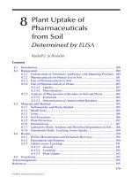
Referring to Figure 5.1, the initial state of the suspension is characterized by
initial values for average size and fractal dimension of the primary particles. Here,
fractal dimension refers to either D
2
or D
3
, and size refers to the longest dimension
for an aggregate. As particles collide and stick, average size increases and fractal
dimension decreases, according to processes discussed earlier in this section. For
example, following a successful collision (i.e., one that results in the two particles
sticking), the resulting volume is larger than the sum of the volumes of the two
colliding particles, as additional pore space is incorporated in the aggregate.
As the process continues, both growth and breakup occur, but growth is faster.
Eventually, a state, represented by point A in Figure 5.1, is reached in which there is
a temporary balance between growth and breakup. During this period there may be

some restructuring of the aggregates, as particles and clusters penetrate into the pore
spaces of larger aggregates, not necessarily increasing size appreciably, but increasing
A
Pr
frac
ag
equilib rium
Fractal dimension
Length, l
A
Primary particle size
Primary particle
fractal dimension
Aggregation
≈ equilibrium
Restructuring,
compaction
breakup,
Time
FIGURE 5.1 Conceptual model of temporal changes in fractal dimensions and average size
(characteristic length) during initial stages of an aggregation process.
Copyright 2005 by CRC Press
“L1615_C005” — 2004/11/19 — 18:48 — page 103 — #9
Effects of Floc Size and Shape in Particle Aggregation 103
density, with a corresponding reduction in fractal dimension. With additional time,
aggregates become more compact and average size may even decrease slightly, as
particles and clusters that are only loosely joined break off and rejoin other aggregates
in a more stable manner. The overall effect is a slight reduction in average size and a
slight increase in fractal dimension. These changes also are illustrated with the floc
sketches at the bottom of Figure 5.1.

The length of time in the initial phase (before point A) will vary, depending on
chemical and mixing conditions, as well as the initial state of the suspension. In the
experiments reported below, this phase lasts approximately 40 to 60 min. In a typical
treatment process, the length of time allowed for mixing is on the order of several
tens of minutes, so the later processes of restructuring and compaction are probably
not significant. In natural systems particular conditions may last longer, and there is
a greater chance particles will be in a near-equilibrium state.
5.3 EXPERIMENTAL SETUP
5.3.1 I
MAGE ANALYSIS
Three sets of experiments were conducted in this study (Table 5.2), each one using an
image-based analysis of aggregates. A nonintrusive imaging technique was used to
capture images of aggregates and toanalyze changes in aggregate properties with time.
Using this technique, aggregates could be maintained in suspension and images were
captured without sample extraction or any other interruption of the experiment. In one
set of tests (Experiment Set 1, Section 5.3.2.1), the images were taken of the mixing
jar containing suspensions immediately at the end of the flocculation step, assuming
the particle shape and size did not change during the settling period. In another set of
TABLE 5.2
Summary of Experiments
Experiments Coagulant Measurements
Shear rate
(sec
−1
)
Experiment Set 1
(lake water and
montmorillonite)
Alum Initial conditions,
charge

neutralization,
sweep floc
n/a-tested
supernatant after
mixing (during
settling)
Experiment Set 2
(latex particles)
(Expts. 1–8)
Alum 10, 20, 30 min 20, 80
Experiment Set 3
(latex particles,
Buffalo River)
(Expts. 9–11)
Polymer 2–150 min 10, 40, 100
Copyright 2005 by CRC Press
“L1615_C005” — 2004/11/19 — 18:48 — page 104 — #10
104 Flocculation in Natural and Engineered Environmental Systems
experiments (Experiment Set 2, Section 5.3.2.2), images were taken from the sample
while slow mixing was still in progress, that is, particles were photographed in situ.
A schematic of the general experimental setup is shown in Figure 5.2. Images of
the suspended particles were illuminated by a strobe light, which provided a coherent
backlighting source. Depending on conditions for a particular experiment, the strobe
pulse rate and intensity were adjusted to produce one pulse during the time the camera
shutter was open. The projected images were captured by a computer-controlled CCD
camera (Kodak MegaPlus digital camera, model 1.4) placed on the opposite side of
the mixing jar from the strobe. Generally the shutter exposure time was between about
80 and 147 ms. The camera captured digital images on a sensor matrix consisting
of 1320 (horizontal) × 1035 (vertical) pixels. Each pixel was recorded using 8 bit
resolution, that is, with 256 gray levels. For the present tests, a resolution of 540 pixels

per mm was achieved. This was determined by imaging a known length on a stage
micrometer and counting the number of pixels corresponding to that length. The cam-
era was mounted on a traversing device so that it could be moved in each of the three
coordinate directions, and images were stored on the hard drive of a PC. Camera
settings were varied to obtain the best quality (greatest contrast between aggreg-
ates and background) for each set of experimental conditions (see Chakraborti
25
for
further details), but pixel resolution was held constant throughout the tests. Pixel
resolution was always sufficient to adequately describe the smallest particles in these
experiments.
26
Experiments were conducted in a darkened room to eliminate light
contamination.
Once saved, images were processed using a public domain image analysis soft-
ware program (NIH Image). Processing steps included contrast enhancement and
thresholding, resulting in a binary image consisting of solids (black) and background
(white). Image was then applied to calculate basic geometric properties for each
aggregate in the image, which included perimeter and area. In addition, an ellipse
was fitted to each aggregate, by matching moment of inertia and area of the original
aggregate. This step resulted in the definition of major and minor ellipse axes, and
the major axis was taken as the characteristic (longest) length, l, of the aggregate.
In order to estimate volumes to calculate D
3
(Equation (5.1)), the two-dimensional
fitted ellipse was rotated about the long axis. As shown by Chakraborti et al.,
27
Strobe light
Meter (pulses/min)
Pulse control

CCD camera
Suspended particles
FIGURE 5.2 Experimental setup consisting of strobe light, CCD camera attached to a
computer, and the suspended sample in a mixing jar.
Copyright 2005 by CRC Press
“L1615_C005” — 2004/11/19 — 18:48 — page 105 — #11
Effects of Floc Size and Shape in Particle Aggregation 105
this procedure produces estimates of volume that are preferable to using a spherical
encased volume assumption, although there is stillobviously greater uncertainlyin the
volume estimates than in the calculations based on area. Since direct measurements
of volume using an image-based method are not available, the ellipse approximation
provides a reasonable approach. After application of Image, all data were transferred
to a spreadsheet for further processing, including calculations of size distributions,
fractal dimensions, and other parameters as described in the following paragraphs.
Before conducting the aggregation experiments, preliminary tests wereconducted
to ensure that the imaging procedures were providing accurate data. Monodisperse
suspensions of several different latex particle sizes with known concentration were
photographed to determine the accuracy of size analysis and also to evaluatethe degree
to which concentration could be reproduced. Initial experiments were conducted by
Cheng et al.,
28
who showed that both 10 µm and 6 µm monodisperse latex solutions
were correctly analyzed. Chakraborti
25
conducted additional tests and, in addition,
used the known concentration to evaluate the sampling volume, defined by the field
of focus of the camera. The sampling volume was found to be approximately 20 mm
square and 3 mm deep. In addition, he conducted a number of sensitivity analyses to
further refine the imaging procedures and evaluate the accuracy and reproducibility
of the imaging results.

5.3.2 MATERIALS AND GENERAL PROCEDURES
Three sets of experimentswere designed to provide data for analysis of particles result-
ing from coagulation and flocculation under different process conditions (Table 5.2).
In these experiments, alum and polymer were used as coagulants. InExperiment Set 1,
particle size distributions and morphology of aggregates obtained from lake water
samples and laboratory suspensions of montmorillonite clay were measured. Results
of these experiments were reported previously,
27
and they demonstrated that fractal
dimension could be used to characterize different stages of aggregation, ranging from
initial untreated suspensions, to conditions of sweep floc with relatively large alum
dose. Experiments were conducted to test the hypothesis that charge neutralization
and sweep floc mechanisms produce fundamentally different particle characteristics,
including differences in fractal dimension. In Experiment Set 2, images of aggregates
were obtained while the suspension was still being stirred during flocculation. Results
demonstrated that images could be obtained in situ and also provided direct observa-
tion of temporal changes in floc characteristics during mixing. Again, alum was used
as a coagulant. The goal of these experiments was to test the hypothesis that changes
in fractal dimension are correlated with the physicochemical conditions of a partic-
ular experiment. These experiments were reported by Chakraborti et al.
26
The third
set of experiments was designed to provide a description of the aggregation process
over longer periods of time for both inorganic and natural suspensions. Polymer was
used as coagulant, to avoid additional mass that may be introduced by alum particles
and to focus on fundamental aggregate growth due to primary particles only. The
previous flocculation experiments were restricted to durations of only 30 min. For
treatment plant operation this length of time may be relevant, but the aggregates were
probably still undergoing changes in their shape and size. In particular, disaggregation
Copyright 2005 by CRC Press

“L1615_C005” — 2004/11/19 — 18:48 — page 106 — #12
106 Flocculation in Natural and Engineered Environmental Systems
and restructuring were relatively unimportant during this earlier period, and become
more important only for longer times. Results from the second and third sets of
experiments provided the basis for model conceptualization and model development
described above. Because Experiment Sets 1 and 2 have been previously reported,
they are only briefly summarized here.
5.3.2.1 Experiment Set 1
Water samples were collected from a shallow lake located on the campus of the
University at Buffalo, Buffalo, New York. The lake has an average depth of 3 m, with
maximum depth of 8 m and a total area of 243,000 m
2
. Experiments also were con-
ducted for clay suspensions prepared by adding montmorillonite clay powder (K-10)
to deionized water to produce a sample with a solids concentration of 100 mg/l. Mont-
morillonite is an aluminum hydrosilicate where the ratio between SiO
2
and Al
2
O
3
is approximately 4 to 1. It has a bulk density of 370 g/l, surface area of 240 m
2
/g
and pH 3.2 observed at 10% suspension (Fluka Chemicals, Buchs, Switzerland). For
coagulant, a stock solution of alum was prepared by dissolving Al
2
(SO
4
)

3
·18 H
2
O
(Fisher Scientific, Pittsburgh, PA) in deionized water to a concentration of 0.1 M
(0.2 M as aluminum). Standard jar tests were conducted with these samples to determ-
ine an appropriate dose of alum to generate a “sweep floc” condition. Changes of
both surface charge (measured as zeta potential) and residual turbidity with alum
dose also were measured. After addition of alum, the suspension was mixed rap-
idly (@∼100 rpm) for 1 min and then slow-mixed for 20 min with a mean velocity
gradient, G = 20 sec
−1
. The mixing was then stopped and images of the resulting
aggregated particles in suspension were taken. All experiments were conducted at
room temperature (∼20
◦
Cto23
◦
C), and the analyzed images were obtained with an
alum dose of 20 mg/l, and with pH maintained at 6.5 by manual addition of acid or
base as required.
5.3.2.2 Experiment Set 2
Monosized polystyrene latex microspheres with a density of 1.05 g/ml (Duke
Scientific Corporation, Palo Alto, CA, United States) were used as the primary
particles for these experiments. The nominal particle diameter was 9.975 µm,
with a standard deviation of ±0.061 µm. Particles were taken from a 15 ml
sample of aqueous suspension with 0.2% solids content (manufacturer’s specific-
ation). The number concentration of particles in the concentrated suspension was
3.66 ×10
6

particles/ml (±10%). Aliquots of 0.06 ml or 0.1 ml of the suspension
were added to the mixing jar along with1lofdeionized water, resulting in ini-
tial number concentrations of 220 and 366 particles/ml, respectively. The higher
and lower concentrations yielded total suspended solids of 0.12 and 0.20 mg/l. The
images were analyzed to track changes in aggregate morphology for a given test,
as well as differences between tests resulting from varying coagulant (alum) dose,
particle concentration and mixing speed, or shear rate.
A freshly prepared stock solution of alum was prepared for each test as in
Experiment Set 1. For each test, after addition of coagulant and an initial rapid
Copyright 2005 by CRC Press
“L1615_C005” — 2004/11/19 — 18:48 — page 107 — #13
Effects of Floc Size and Shape in Particle Aggregation 107
mixing period (with G = 100 sec
−1
) for 1 min, the mixing speed was reduced to
either G = 20 sec
−1
or G = 80 sec
−1
and continued until the end of the experiment.
All tests were conducted at room temperature (20
◦
Cto∼23
◦
C) and a constant pH of
6.5 was maintained by adding acid or base as required. Measurements were taken at
10, 20, and 30 min after the initial rapid mixing period. Experiments were performed
to evaluate temporal changes in the fractal dimensions of aggregates formed dur-
ing flocculation of the microspheres. Particle size distributions, collision frequency,
and aggregate geometrical information at different mixing times were obtained under

variable conditions.
5.3.2.3 Experiment Set 3
Typically, two types of suspension were used in the third set of experiments: abiotic
(latex) and natural (collected from alocal river), containingboth inorganic and organic
constituents. These experiments were conducted using the same equipment and gen-
eral procedures as in Experiment Sets 1 and 2. Polystyrene latex particles (Duke
Scientific Corporation, Palo Alto, CA) of 6 µm diameter (6.038 µm ± 0.045 µm;
density 1.05 g/ml) with a particle concentration of 4000 /ml were used as the primary
particles for the abiotic suspensions. Suspensions were prepared by adding a pre-
determined quantity of particles in deionized water and stirring vigorously to insure
homogeneity. These solutions contained 4.52×10
−5
% solids by volume, or 0.5 mg/l.
A constant pH = 6.5 was maintained by adding acid or base as required.
The natural suspension was obtained from the Buffalo River (Buffalo, New York).
This sample was collected at about 0.5 m below the water surface at a point where the
channel is about 50 m wide and total water depth is about 7 m (in the mid-section).
The wind velocity recorded on the sampling day was 27 kmph (17 mph), and water
temperature was 10.55
◦
C (51
◦
F). The organic content was measured by oven drying
a filtered 500 ml sample for 24 h at 105
◦
C, followed by 24 h of oven drying at 550
◦
C.
The measured total solids content (TSS) was 14.6 mg/l (measured using a 0.22 µm
filter), which is fairly typical for rivers, and the volatile organic solids (VSS) was

0.4 mg/l, resulting in a 2.74% organic content.
Since the surface charge of suspended particles is negative, cationic polymer
was used for coagulant. Polymer was chosen since it does not form gel or add
particles in suspension like alum floc, and it allows quick aggregation. Alken solu-
tions (Alken-Murray Corporation, New York) supplied the polymer Ethanediamine
(C193K) for these experiments. This polymer has a molar mass less than one million
(∼700,000) and contains the quaternary amine (ammonium) group that produces the
positive charge. According to the manufacturer, it is completely soluble and has an
effective pH range of 0 to 13, with good floc formation at solution pH between 4 and 6.
Fresh polymer (0.5% stock solution, per manufacturer’s specifications) was prepared
for each experiment, and the solution was shaken vigorously before each use.
The selected mixing speeds for the experiments were 15 rpm, 46 rpm, and
100 rpm, resulting in average velocity gradients, G = 10 sec
−1
, 40 sec
−1
, and
100 sec
−1
, respectively. These values were chosen to span the range of mixing
environments found in engineered and natural aquatic systems, although some natural
environments may have even lower mixing intensities. For each experiment, samples
Copyright 2005 by CRC Press
“L1615_C005” — 2004/11/19 — 18:48 — page 108 — #14
108 Flocculation in Natural and Engineered Environmental Systems
were rapid mixed for 1 min to provide thorough mixing of the particles with the
coagulant. The stirring rate was then adjusted to the desired level and images of the
flocs were taken at different times throughout the experiment.
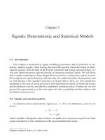
Preliminary tests were performed to determine the quantity of coagulant needed
to produce particle aggregation at the desired rate. Measurements of zeta potential and

resulting residual turbidity (measured at 30 min after stopping the mixing) are shown
in Figure 5.3 for different polymer doses added to Buffalo River suspensions. Basic
stages of aggregation may be seen with increasing coagulant dose. Initially (Stage I),
particle surface charge is reduced as the particles become destabilized. The principle
aggregationmechanism inthis stage is thereduction of electrostaticrepulsion between
particles as a result of surface charge reduction. Charge neutralization (Stage II) is
reached when sufficient coagulant is added so that the originally negatively charged
particles are just neutralized, and aggregates are formed when contacts occur. Further
addition of coagulant leads to charge reversal and restabilization (Stage III) where
aggregation is not chemically favored. When alum is used as coagulant, Al(OH)
3
(s)
is produced, which coats particles with a gelatinous and “sticky” sheath. At higher
doses and for appropriate pH range, “sweep floc” may occur, which causes aggregates
to settle more quickly and reduce turbidity. This stage is not present for the polymer,
which does not produce “sweep floc.”
As the surface charge of the suspended particles changes with increasing coagu-
lant dose, the resulting residual turbidity decreases, reaching a minimum for a dose
near the dose correspondingto neutralsurface charge (Figure 5.3). The initial turbidity
for the Buffalo River suspension was 28 NTU, and the coagulant dose causing charge
neutralization was 520 µg/l. For doses higher than the neutral surface charge dose,
–6
–4
–2
0
2
4
6
200
Stage I

Stage II
Stage III
400 600 800 1000 1200 1400
0
5
10
15
20
25
30
Polymer dose (g/L)
Turbidity
Zeta pot.
Zeta potential (mV)
Residual turbidity (NTU)
16000
FIGURE 5.3 Zeta potential and residual turbidity measurements as a function of coagulant
dose for Buffalo River suspension; different stages of aggregation are indicated with increasing
dose.
Copyright 2005 by CRC Press
“L1615_C005” — 2004/11/19 — 18:48 — page 109 — #15
Effects of Floc Size and Shape in Particle Aggregation 109
turbidity increases slightly. Once the dose of coagulants was selected for a partic-
ular experimental condition (the charge neutralization dose), the next step was to
photograph and analyze images of particles from the mixing jar, as described above.
5.4 RESULTS AND DISCUSSION
5.4.1 O
BSERVATIONS AND ANALYSIS OF DATA
5.4.1.1 Coagulation–Flocculation
A time series of floc images formed by Buffalo River particles at different mixing

times is shown in Figure 5.4 (these images were obtained as a prelude to the tests in
Experiment Set 3). After only 2 min, the initially monodispersed particles are seen
to form flocs of various shapes and sizes, and larger flocs formed with additional
time. The larger aggregates at later times appear to be more porous and spread out
than the smaller aggregates observed at earlier times, and are associated with lower
fractal dimensions. The images show that the aggregate structure is an agglomer-
ate of particles/clusters, with a highly irregular surface. Qualitatively at least, this
observation supports the characterization of natural aggregates in terms of fractal
geometry. The series of images in Figure 5.4 also is consistent with the aggregation
2 min 5 min 10 min 15 min 20 min
90 min 120 min 150 min
100 m
30 min 40 min 50 min 60 min
FIGURE 5.4 Images of aggregates from Buffalo River suspensions at different times of
aggregation.
Copyright 2005 by CRC Press
“L1615_C005” — 2004/11/19 — 18:48 — page 110 — #16
110 Flocculation in Natural and Engineered Environmental Systems
stages described in Figure 5.1. During the initial period of coagulation, aggregates
quickly grow and become more convoluted and porous. Later, after about 50 or
60 min, aggregates appear to be more regular, with a smoother surface. This condi-
tion corresponds with the later stages described in Figure 5.1, where more loosely
bound clusters have been broken off and the aggregates become denser as inner pore
spaces become occupied. The period between about 40 and 60 min shows only minor
changes, which should correspond with the state indicated around point A in Fig-
ure 5.1. For times greater than about 90 min, the aggregate size seems to decrease
slightly, again consistent with the later stages described in Figure 5.1.
5.4.1.2 Particle Size and Shape
Geometric information from the image analysis was used to characterize particles.
Temporal changes in aggregate size distribution for experiments with latex particles

mixed with G = 20 sec
−1
and G = 10 sec
−1
are shown in Figure 5.5, where fre-
quency of occurrence (number) in each size class is plotted against the aggregate
characteristic length (major ellipse axis) using a logarithmic scale. Test results using
alum (Experiment Set 2) and polymer (Experiment Set 3) are shown. In both cases
the gradual movement of the peak of the distribution toward larger size is clearly
seen, indicating that aggregate growth was the primary mechanism during this period
(also shown in Figure 5.4). In this period (0 to 30 min) conditions are such that
the model of Equation (5.10) is applicable, that is, breakup is negligible. Compared
with the results using polymer, alum treatment seems to result in more peaked size
distributions, with less spread about the mode. The peak size for the polymer treated
experiment showed a more significant increase with time and the peak had smaller
magnitudes than with the alum treated test. The higher peak associated with the alum
0
5
10
15
20
25
30
35
40
0.5 1 1.5 2 2.5
10 min (Alum)
20 min (Alum)
30 min (Alum)
10 min (Poly)

20 min (Poly)
30 min (Poly)
Log l
Relative frequency (%)
FIGURE 5.5 Temporal plot of particle size distribution for latex suspensions mixed at G =
20 sec
−1
using alum, and mixed at G = 10 sec
−1
using polymer (Poly).
Copyright 2005 by CRC Press
“L1615_C005” — 2004/11/19 — 18:48 — page 111 — #17
Effects of Floc Size and Shape in Particle Aggregation 111
treated tests may be related to additional solids added by the alum, and to different
particle concentrations used in the two sets of experiments. It is difficult to com-
pare the two suspensions directly since different coagulants were used and the zeta
potentials for the two suspensions at charge neutralization were different, as were the
mixing speeds. Keeping these differences in mind, the polymer treated coagulation
produced larger (and possibly stronger) particles more quickly than coagulation by
alum at the charge neutralization stage.
Temporalchanges in the peak of the particle size distributionfor BuffaloRiver sus-
pensions mixed with polymer at G = 10 sec
−1
are illustrated in Figure 5.6. The peak
size gradually increases (until about 50 to 60 min) and then it decreases. The decrease
at later times is thought to be due to the breakup effect, which has been described in
several previous studies. For example, Williams et al.
29
reported a breakup of particle
size after reaching a peak for silica particles mixed at various speeds. Their study

suggested that smaller G would induce a larger peak and a relatively smaller decrease
of peak size over time, compared to a higher mixing rate. A similar observation was
reported by Selomulya et al.,
30
who found that the average aggregate size (for latex
particles) decreased with time after reaching a peak, using a range of shear rates (40
to 80 sec
−1
).
Further evidence of this type of behavior is seen in Figure 5.7 and Figure 5.8,
where temporal changes in median aggregate size and D
2
are plotted for both latex
(LT) and Buffalo River (BR) suspensions treated with polymer under three different
mixing rates. Although not shown here, similar results were found with D
3
as with
D
2
. In general, slower mixing produced larger aggregates (Figure 5.7) and lower D
2
(Figure 5.8) for both these experiments, and changes in the Buffalo River suspensions
were relatively more pronounced. This may be due to higher solids concentration for
the Buffalo River suspension, or to the presence of organic material, which was not
a factor in the latex tests. In addition, there was greater heterogeneity in aggregate
size and shape for Buffalo River suspensions. In both cases there is a gradual increase
in size and decrease in D
2
, followed by the attainment of approximately steady-state
5 10203040506090120

50
100
150
200
250
0
300
l
max
(m)
2 150
Time (min)
FIGURE 5.6 Temporal change in the peak of the particle size distribution for Buffalo River
suspensions mixed at G = 10 sec
−1
.
Copyright 2005 by CRC Press
“L1615_C005” — 2004/11/19 — 18:48 — page 112 — #18
112 Flocculation in Natural and Engineered Environmental Systems
10
15
20
25
30
35
10 s
–1
(LT) 40 s
–1
(LT) 100 s

–1
(LT)
10 s
–1
(BR) 40 s
–1
(BR) 100 s
–1
(BR)
l (m)
5
40
20 40 60 80 100 120 140
Time (min)
0 160
FIGURE 5.7 Temporal changes in the particle size (median) for latex (LT) and Buffalo River
(BR) suspensions with various shear rates.
20 40 60 80 100 120 140
Time (min)
0 160
2
1.8
1.6
1.4
2.2
1.2
D
2
10 s
–1

(LT) 40 s
–1
(LT) 100 s
–1
(LT)
10 s
–1
(BR) 40 s
–1
(BR) 100 s
–1
(BR)
FIGURE 5.8 Temporal plot of D
2
for experiments with latex (LT) and Buffalo River (BR)
suspensions with 10 sec
−1
, 40 sec
−1
and 100 sec
−1
mixing speeds.
values. The final steady-state size was found to be higher than the initial size, but
lower than the peak size, and final D
2
was lower than the initial value, but higher than
the minimum, consistent with the above conceptual model description (Figure 5.1).
The effect of mixing speed, suggested in the results of Figure 5.7, is further
demonstrated in Figure 5.9, whereaggregate area is plotted as a function of size for two
experimentsfrom ExperimentSet 2, using a relativelyhigh anda relativelylow mixing

speed. The slopes for the lines (estimated as D
2
— see Equation (5.1)) corresponding
to G = 20 sec
−1
and G = 80 sec
−1
were 1.62 (±0.02)and 1.75 (±0.03), respectively,
where the ± values are the standard errors for the regression lines. The results verify
that aggregate size correlates with mixing speed (and fractal dimension), with smaller
size corresponding to larger G and larger D
2
. For comparison, lines with D
2
= 1 and
Copyright 2005 by CRC Press
“L1615_C005” — 2004/11/19 — 18:48 — page 113 — #19
Effects of Floc Size and Shape in Particle Aggregation 113
100
10000
1000
10
100000
A
(

m
2
)
100

10
l (m)
1 1000
D
2
=2
D
2
=1
80 sec
–1
20 sec
–1
FIGURE 5.9 Effect of shear rate (G = 20 sec
−1
and 80 sec
−1
) on aggregate size, as
represented by area, and comparison with Euclidean relationship (D
2
= 2).
D
2
= 2 also are drawn in Figure 5.9. With all data points falling between these two
lines, it is clear that the aggregate size depends on a fractal relation.
5.4.1.3 Density and Porosity
Solid density and porosity for aggregates produced in Experiment Set 1 at sweep
floc condition were calculated using Equations (5.4) and (5.5) and plotted as func-
tions of aggregate size, taken as the major axis of the ellipse fitted to each aggregate
(Figure 5.10). Various parameters needed in thesedefinitions (e.g., shapefactors) were

evaluated using the imaging technique.
18,31
Primary particle density was assumed to
be 2.65 g/cm
3
, corresponding to clay or silt particles. For larger aggregates, large
portions of the aggregate contained pores, with porosity varying between 0.92 and
0.99. Floc density varied from 1.01 to 1.10 g/cm
3
, considerably less than the primary
particle density. Curves were fit to the data for porosity and density, along with cor-
responding data from Amos and Droppo.
32
As shown in Figure 5.10, the smoothness
of the fit for these curves indicates that aggregate properties scale with size. A similar
relationship between floc size, density, and porosity has been observed in several pre-
vious studies.
5,33,34
As previously noted, these properties are important for settling
and general transport calculations.
5.4.1.4 Collision Frequency Function
Collision frequency (β) was calculated using relations summarized in Table 5.1.
To illustrate the general results, β values for a latex suspension mixed with G =
20 sec
−1
and treated with alum are shown in Figure 5.11. Results for other tests
and other particle size combinations showed similar trends and are not shown here
(see Chakraborti
25
for further details). To calculate collision frequency functions, two

particle sizes (i and j) are required. In these calculations, the primary particle size was
taken as 10 µm, and different sizes for the second colliding particle were assumed,
varying between 10 µm and 1 mm. Results also are shown when variable fractal
Copyright 2005 by CRC Press
“L1615_C005” — 2004/11/19 — 18:48 — page 114 — #20
114 Flocculation in Natural and Engineered Environmental Systems
Density, Amos & Droppo
Porosity, Amos & Droppo
Porosity, this study
(a)
(b)
Density, this study
1.1
1.05
1
0.95
0.9
0.85
35030025020015010050
Density (gm/cm
3
)
1.15
0.8
4000
l (m)
l (m)
0.96
0.92
0.88

0.84
400350300250200150100500
Porosity
1.00
0.80
FIGURE 5.10 Aggregate properties as a function of size for lake water suspensions and
measurements by Amos and Droppo
32
for (a) density and (b) porosity. Bars represent the
observed range of data.
dimensions are used. In this case, the fractal dimensions obtained from Experiment
Set 2, corresponding to the three different measurement times, were incorporated
in the calculations (D
2
= 1.84, 1.75, and 1.65, and D
3
= 2.77, 2.62, and 2.47, for
t = 10 min, 20 min, and 30 min, respectively). As expected, the effects of shear
rate and differential sedimentation were much greater than the effects of Brownian
motion. Furthermore, except for the largest particles, the impact of shear rate was
greater than differential sedimentation.
Noting that the fractal dimensions decreased with time, it is seen that β generally
increased with time during these experiments. The increase is particularly evident
for colliding particles larger than about 100 µm, where nearly an order of magnitude
Copyright 2005 by CRC Press
“L1615_C005” — 2004/11/19 — 18:48 — page 115 — #21
Effects of Floc Size and Shape in Particle Aggregation 115
1.0E – 02
1.0E – 04
1.0E – 06

10 100 1000
l (m)
1.0E + 00
1.0E – 08
 (cm
3
/sec)
20 min
30 min
10 min
FIGURE 5.11 Total collision frequency (β) as a function of particle size (l) at different times
of aggregation for latex suspensions mixed at G = 20 sec
−1
.
10
1
100
 (D)/
(3)
10 100 1000 10000 1000001 1000000
vj/vi
20 min
30 min
10 min
FIGURE 5.12 Comparison of total collision frequency function calculated according to
fractal (β(D)) and Euclidean (β(3)) formulas at different times of aggregation.
increase is seen in the values of β for the fractal dimension corresponding to 30 min,
relative to the values for 10 min. This is due to the effect of larger collision radii
for aggregates that sweep out a larger volume and provide greater opportunity for
collisions with other particles.

It also should be noted that the β values shown in Figure 5.11 are significantly
greater than the values that would be calculated based on Euclidean dimensions. For
example, setting D
2
= 2 and D
3
= 3 in the formulas in Table 5.1 gives β values
consistent with traditional models that assume spherical particles. A comparison of β
calculated using the Euclidean values (β(3)) and β from the fractal formulas (β(D))
is shown in Figure 5.12, where it can be seen that order of magnitude and greater
increases are obtained using the fractal calculations. Chakraborti
25
provides a more
detailed comparison of different calculation results for a range of particle sizes.
Copyright 2005 by CRC Press
“L1615_C005” — 2004/11/19 — 18:48 — page 116 — #22
116 Flocculation in Natural and Engineered Environmental Systems
5.4.1.5 Settling Velocity
Using results from Experiment Set 1, the exponent in Equation (5.9) was found to
be 1.96 for initial conditions, 1.73 at the charge neutralization dose, and 1.47 for
sweep floc, for the lake water samples. Corresponding values for the montmorillonite
suspensions were 1.82, 1.70, and 1.62, respectively. Although the exponent in these
results becomes smaller for higher alum dose, l also increases with each success-
ive coagulation stage, suggesting more rapid collision rates.
35
Thus, larger aggregate
size appears to offset the effect of lower fractal dimension and helps to explain the
common observation from water treatment practice that sweep coagulation results in
better (lower turbidity water) settling than charge neutralization.
However, in order to fully evaluate settling, the aggregate density also must be

taken into account. With increasing size (l), results from Figure 5.10(a) show that
density decreases, which should reduce w
s
(Equation (5.9)). Calculations based on
the present samples show that w
s
increases with increasing l, but at a slower rate
than would be expected using a traditional (Stokes-based) model (Figure 5.13). Data
in this figure were obtained by taking images of samples from the Buffalo River,
which were allowed to passively settle in the mixing jar. The images were double
exposed so that each aggregate was pictured twice. The difference in locations of
each of the aggregate pairs was then divided by the known time interval between
the two images to obtain settling rate. These rates were then plotted as a function
of aggregate size. The best fit line drawn through the data has w
s
∝ l
1.30
, an expo-
nent value clearly less than 2 and, in fact, even less than the exponent suggested
in Equation (5.9) (discussed earlier). Thus, an additional factor must be affecting
the settling, which may be due to changes in density or changes in the drag coeffi-
cient, as previously suggested. The net effect of these various factors is unknown
in general, and further data are needed to determine the correct relationship for
settling.
100
200
300
400
500
W

s
(m/sec)
0
600
51015
l (m)
020
Measured
Stokes
FIGURE 5.13 Settling velocity of Buffalo River solids.
Copyright 2005 by CRC Press
“L1615_C005” — 2004/11/19 — 18:48 — page 117 — #23
Effects of Floc Size and Shape in Particle Aggregation 117
5.5 CONCLUSIONS AND RECOMMENDATIONS
The focus of this study is on developing relationships between aggregate size and
shape, and transport and growth behavior. Experiments were conducted to demon-
strate the dependence of aggregate properties on fractal dimensions, consistent with
the supposition that improvements could be made in describing aggregate character-
istics and behavior in aqueous solutions using a fractal-based analysis, rather than
relying on the common approach of assuming the aggregates are impervious spheres.
An image-based analysis was used to develop basic geometrical properties of aggreg-
ates in suspension, from which properties such as fractal dimension could be derived.
Basic properties suchas density and porosity were shownto be functions of size, which
also was correlated with fractal dimension. Along with relatively high porosity, these
results show that the solid sphere assumption has obvious drawbacks, although it
clearly has facilitated progress in aggregation theory.
To develop a full model of particle transport and behavior in an aqueous system,
an extended version of Equation (5.10) would serve as a reasonable starting point,
with additional terms added according to the needs of a particular application. Those
terms might include breakup, settling, and internal reactions, or sources and sinks of

material. The present experiments were designed to shed light on the particle aggreg-
ation and settling mechanisms, and although progress has been made, the results here
are far from complete. For example, there is still uncertainty in the volume calcula-
tions, and methods are needed for nonintrusive measurement of aggregate volume.
Much work remains to be done to complete a full model description, particularly with
respect to settling.
From a modeling point of view, an approach needs to be developed that can
incorporate changes in fractal dimensions directly into the aggregation modeling
framework (Equation 5.10). Once fractal dimensions are known, they can be used to
calculate collision frequencyfunctions (Table5.1) which are needed in theaggregation
calculations. Experimental results were shown to be consistent with the conceptual
model, and indicated that the basic Smoluchowski approach (Equation 5.10) could
still be used, but that collision frequencies should be updated as functions of time, as
fractal dimensions change. For the present tests fractal dimensions were supplied to
the model using a simple empirical fit to the observed data, but ideally these values
would be developed in a separate submodel. At this stage, the only approach available
to accomplish this is with a DLA or RLA-type model, which would account for each
individual aggregate (or at least some representative number of aggregates) and keep
track of changes in fractal dimensions. While theoretically appealing, this approach is
at best cumbersome for general modelingpurposes, andis computationally unrealistic,
even with today’s computer capabilities. Nonetheless, as a research tool, this type of
model may be useful and is worth a more detailed look.
Values for β are considerably different when fractal dimensions are taken into
account, andan unexpected result of incorporating better resolvedβ in the calculations
has been the realization of the need for further evaluation of α, in particular as a time-
varying parameter that depends not only on the chemistry of the solution and the
surface of the aggregate, but also on aggregate structure. In other words, noting
that α is generally used as a fitting parameter, and that aggregation is controlled
Copyright 2005 by CRC Press
“L1615_C005” — 2004/11/19 — 18:48 — page 118 — #24

118 Flocculation in Natural and Engineered Environmental Systems
by the product of α and β, then changes in β suggest that corresponding changes
in α will be required. In addition, since β changes with time, it may be expected
that α should change with time. This makes intuitive sense, as the likelihood of two
colliding aggregates sticking together should be greater when they have a rougher
surface, compared with a smooth sphere. So far, very little research has been directed
at a finer description of collision efficiency, and this is an important area for further
improvement of aggregation models.
The conceptual model developed here has been useful in explaining the different
stages of aggregation for the present experiments and, more importantly, the rela-
tionship between fractal dimensions and different aggregation processes. Although
designed with the specific conditions of the present experiments in mind, the model
provides a framework within which one may conceptualize the correspondence
between fractal dimensions and physical changes occurring among the aggregates.
The model is easily extended to consider situations where an initially monodisperse
suspension is not required, as the basic ideas are also applicable when a change in
mixing or chemistry is induced in a system where at least the initial size distribution
is known.
A property of particular interest is the settling rate, and results shown in
Figure 5.13 indicate that Stokes’ law is inadequate for estimating settling for fractal
aggregates. Particular problems with the application of Stokes’ law include determin-
ation of appropriate aggregate size and density, as well as the assumption of laminar
flow around the aggregate, and the associated formulation of the drag coefficient.
This last point also applies for the fractal-based expression (Equation (5.9)), since the
correct formulation for drag coefficient has not been demonstrated, only assumed.
The results shown in Figure 5.13 suggest the dependence of w
s
on l is different than
in Equation (5.9), and this difference may be due to an inadequate description of
the drag coefficient. The drag coefficient assumed in Equation (5.9) comes from the

expression for a sphere in laminar flow, but it would be more consistent to assume
C
D
as a function of fractal dimensions, which characterize general aggregate shape
and would introduce the impact of different shapes on settling characteristics. Along
with collision frequency and efficiency, this is another specific area where fractal
dimensions can improve our ability to model particle aggregation and behavior in
suspensions.
NOMENCLATURE
A Projected area
C
D
Drag coefficient
D
1
One dimensional fractal dimension
D
2
Two dimensional fractal dimension
D
3
Three dimensional fractal dimension
g Gravitational constant
G Shear rate
k
B
Boltzmann constant
l Object characteristic length
Copyright 2005 by CRC Press
“L1615_C005” — 2004/11/19 — 18:48 — page 119 — #25

Effects of Floc Size and Shape in Particle Aggregation 119
m Mass
m
s
Solid mass (in an aggregate)
n
i
Number of particles, i-th size
N Number of primary particles
P Perimeter
Re Particle Reynolds number
t Time
T Absolute temperature
V Volume
w
s
Settling velocity
α Collision efficiency
β Total collision frequency function
β
Br
Collision frequency function due to Brownian motion
β
Sh
Collision frequency function due to shear rate
β
DS
Collision frequency function due to differential sedimentation
ρ Density
φ Porosity

ψ Fractal constant
ξ Shape factor
µ Dynamic viscosity
ν Kinematic viscosity
ζ Packing factor
REFERENCES
1. O’Connor, D.J., Models of sorptive toxic substances in freshwater systems. III Streams
and Rivers, J. Environ. Eng., 114 (3), 552–574, 1988.
2. Droppo, I.G. and Ongley, E.D., The state of suspended sediment in the freshwater
fluvial environment: A method of analysis, Water Res., 26 (1), 65–72, 1992.
3. O’Melia, C.R., and Tiller, C.L., Physicochemical aggregation and deposition in aquatic
environments, in Environmental Particles (Vol 2), J. Buffle and H.P. van Leewen, Eds.,
Lewis Publishers, Boca Raton, FL, 1993, chap. 8.
4. Chapra, S.C., Surface Water Quality Modeling, McGraw Hill, New York, 1997.
5. Droppo, I.G., et al., The freshwater floc: A functional relationship of water and organic
and inorganic floc constituents affecting suspended sediment properties, Water Air Soil
Pollut., 99, 43–54, 1997.
6. Lawler, D.F., Removing particles in water and wastewater, Environ. Sci. Technol.,20
(9): 856–861, 1986.
7. Elimelech, M., Gregory, J., Jia, X., and Williams, R.A., Particle deposition and
aggregation — Measurement, modeling and simulation, Butterworth-Heinemann Ltd.,
London, U.K., 1995.
8. O’Melia, C.R., Coagulation, in Water Treatment Plant Design for the Practicing
Engineer, R.L. Sanks, Ed., Ann Arbor Science, MI, 1979, chap. 4.
9. Gregory, J., Fundamentals of flocculation, Crit. Rev. Env. Con., 19 (3), 185–230, 1989.
10. Mandelbrot, B.B., The Fractal Geometry of Nature, W.H. Freeman, San Francisco,
CA, 1983.
11. Meakin, P., Fractal aggregates, Adv. Coll. Int. Sci., 28, 249–331, 1988.
Copyright 2005 by CRC Press