Flocculation In Natural And Engineered Environmental Systems - Chapter 8 docx

“L1615_C008” — 2004/11/19 — 02:48 — page 171 — #1
8
An Example of Modeling
Flocculation in a
Freshwater Aquatic System
Bommanna G. Krishnappan and Jiri Marsalek
CONTENTS
8.1 Introduction 171
8.2 The Stormwater Detention System 172
8.3 Experimental Study 173
8.3.1 Rotating Circular Flume 173
8.3.2 Deposition Tests 174
8.4 Mathematical Model 176
8.5 Application of the Model to the Laboratory Data 178
8.5.1 Input Parameters 178
8.5.1.1 Settling Velocity of the Flocs, w
k
178
8.5.1.2 Turbulent Diffusion Coefficient, D 178
8.5.1.3 Deposition Flux, F
d
179
8.5.1.4 Erosion Flux, F
e
179
8.5.1.5 Collision Efficiency Parameter, β 179
8.5.1.6 Collision Frequency Functions K
b
, K
sh
, K

I
, K
ds
179
8.5.1.7 Model for the Growth-Limiting Effect of Turbulence 179
8.6 Comparision of Model Predictions with the Measured Data 180
8.7 Summary and Conclusions 185
Acknowledgments 186
Nomenclature 186
References 187
8.1 INTRODUCTION
Flocculation in natural freshwater systems has been suggested and inferred by many
researchers,
1–4
and was explicitly investigated by Droppo and Ongley.
5
These studies
and others
6–9
have concluded that in addition to the electrochemical processes, the
bacterial processes also play a role in the formation of freshwater flocs. It is believed
(Ongley et al.
10
) that the biological processes contribute for flocculation in two dif-
ferent ways: bacterial bonding and bacterial “glue.” Marshall
6
had shown that the
1-56670-615-7/05/$0.00+$1.50
© 2005 by CRC Press
171

Copyright 2005 by CRC Press
“L1615_C008” — 2004/11/19 — 02:48 — page 172 — #2
172 Flocculation in Natural and Engineered Environmental Systems
bacteria have a high affinity for fine grained sediment particles and thereby promotes
flocculation by increasing the surface area and bonding two or more mineral particles
together. Biddanda
11
and Muschenheim et al.
8
had shown that secretion of extracel-
lular polymeric exudates by certain bacteria provide the necessary bonding material
(glue) to hold particles together.
Modeling of the flocculation process in freshwater system has been attempted by
several investigators.
12–15
The approach used by these investigators is based on the
premise that the freshwater flocculation is a two step process in which the particles
are first brought into contact by collision mechanisms such as Brownian motion,
laminar and turbulent fluid shear, inertia, and differential settling, and subsequently, a
certain amount of such collisions result in the formation of flocs because of the
electrochemical and bacterial bonding and bacterial “glue.” While our knowledge on
the collision mechanisms and the collision frequencies is reasonably well established,
the same cannot be said for the actual mechanism of flocculation (i.e., how collided
particles bind and form flocs). The approach used in the existing models is to introduce
a collision efficiency parameter that is a measure of the probability of successful
collisions, and to determine the value of this parameter as part of the calibration
process of the model. A flocculation modeling approach proposed by Krishnappan
and Marsalek
15
for a stormwater detention pond is reviewed here to highlight the

current state of knowledge in the area of modeling of freshwater flocculation.
8.2 THE STORMWATER DETENTION SYSTEM
The freshwater system that wasconsideredbyKrishnappanandMarsalek
15
is a storm-
water detention pond in Kingston, Ontario, Canada. The layout of the pond is shown
in Figure 8.1. The pond consists of two cells; a wet pond and a dry pond. The surface
area of each pond is about one half of a hectare. The permanent depth of water in
the wet pond is about 1.2 m. The pond was constructed in 1982 to minimize the
impact of runoff from a newly built shopping plaza on the Little Cataraqui Creek.
Pond
outlet
Weir
Station 9
Weir
Cree
k
inlet
Weir
Parking lot
inflow
Wet pond
Dry pond
025m
N
FIGURE 8.1 Schematic layout of the Kingston Stormwater Detention pond.
Copyright 2005 by CRC Press
“L1615_C008” — 2004/11/19 — 02:48 — page 173 — #3
An Example of Modeling Flocculation in a Freshwater Aquatic System 173
This creek drains an urban catchment with a drainage area of about 4.5 km

2
. Since the
construction of the pond, continued development in the catchment basin has increased
the stream flow and hence reduced the effectiveness of the pond. Ongoing sediment-
ation in the pond has further exasperated the problem. To assess the effectiveness of
the pond to trap sediment, a fine sediment transport study was initiated. As part of this
study, deposited sediment from the pond and the pond water were collected and tested
in a rotating circular flume to ascertain the sediment behavior under different bound-
ary shear stress conditions (Krishnappan and Marsalek
16
). These experiments had
indicated that the pond sediment underwent flocculation when subjected to a flow
field, and consequently the settling behavior of the sediment differed significantly
from that of the constituent primary particles.
Existing methods for analyzing suspended solids settling in stormwater ponds
do not consider flocculation of the sediment, and treat the particles as discrete and
noninteracting particles. Such an approach is not satisfactory, and hence there is a
definite need for a model that would take into account the flocculation process of the
stormwater sediment. To meet this need, Krishnappan and Marsalek
15
formulated a
flocculation and settling model for the Kingston pond sediment. The formulation of
the model was based on their experimental study in the rotating flume for the sediment
from the Kingston stormwater pond.
8.3 EXPERIMENTAL STUDY
Deposited sediment from the pond was collected at a number of sampling stations
within the wet pond using an Ekman dredge and combined to form a composite
sample. The sample and a large volume (500 l) of pond water were brought to
the Hydraulics Laboratory of the National Water Research Institute in Burlington,
Ontario, Canada and were tested in the Rotating Circular Flume. Use of the pond

water as the suspending medium preserved the chemical and biological characteristics
of the sediment–water mixture in the laboratory experiments.
8.3.1 R
OTATING CIRCULAR FLUME
A sectional view of the rotating circular flume is shown in Figure 8.2. The flume is
supported by a rotating platform, which is 7.0 m in diameter. The flume is 5.0 m in
diameter at the centre-line, 30 cm wide, and 30 cm deep. The annular top cover fits
inside the flume with close tolerance. The gap between the edges of the top cover
and the flume walls is about a millimeter. The height of the cover inside the channel
can be adjusted by raising or lowering the top cover. The flume and the cover are
rotated in opposite directions. The maximum rotational speed of both components is
three revolutions per minute. The flume is equipped with a Laser Doppler Anemo-
meter to measure the flow field and a Malvern Particle size analyzer to measure the
size distribution of sediment flocs in suspension. The Malvern Particle size analyzer
was placed directly underneath the flume, and the sampling cell of the instrument was
connected to a short sampling tube that was inserted through the bottom plate of the
flume into the flow. The sample was drawn through the sampling cell continuously
Copyright 2005 by CRC Press
“L1615_C008” — 2004/11/19 — 02:48 — page 174 — #4
174 Flocculation in Natural and Engineered Environmental Systems
10T.Cap. Jackscrew
Annular top plate
support
Annular top plate
Annular channel
Upper deep groove
ball bearing
Outer hollow
drive shaft
Upper main tapered

roller bearing
Inner rotating
solid shaft
Lower main tapered
roller bearing
Slip ring assembly
Lower deep groove
ball bearing
3.5 m
0.30 m
0.30 m
5.0 m
7.0 m
FIGURE 8.2 A sectional view of the rotating circular flume used in the experimental study.
and the instrument was operated in its flow-through mode. The size distribution of
the sediment flocs were monitored at regular intervals of time. The complete details
of the flume and the instruments can be found in Krishnappan.
17
8.3.2 DEPOSITION TESTS
Deposition tests were carried out by placing the pond water and a known amount
of sediment in the flume and operating the flume at the maximum speed to mix the
sediment thoroughly. The amount of sediment added was enough to produce a fully
mixed concentration of about 200 mg/l. The flume and the top cover were operated at
the maximum speed for about 20 min, and then the speed was lowered to the desired
shear stress level. The flume was then operated at this level for about 5 h. During this
time, both suspended sediment concentration and the size distribution of sediment in
suspension were monitored at regular intervals of time.
Figure 8.3 shows the variation of suspended sediment concentration as a function
of time for five different bed shear stress conditions. From this figure, we can see
that after the initial 20-min mixing period, the concentration decreases gradually and

tends to reach a steady state value for all the shear stresses tested. The steady state
concentration is a function of the bed shear stress. From such data, it is possible
to calculate the amount of sediment that would deposit under a particular bed shear
stress under a steady flow condition.
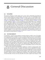
The size distribution data measured during the deposition experiments are sum-
marized in Figure 8.4. In this figure, the median sizes of the distributions are plotted as
a function of time for three of the five deposition tests. For the lowest bed shear stress
Copyright 2005 by CRC Press
“L1615_C008” — 2004/11/19 — 02:48 — page 175 — #5
An Example of Modeling Flocculation in a Freshwater Aquatic System 175
50.00
100.00
150.00
200.00
Bed shear stresses
0.056 N/m
2
0.121 N/m
2
0.169 N/m
2
0.213 N/m
2
0.324 N/m
2
Time (min)
0 50 100 150 200 250 300 350
Concentration in mg/l
0.00
250.00

FIGURE 8.3 Concentration vs. time curves for different shear stresses during deposition.
50 100 150 200 250 300
Median size in microns
0.00
10.00
20.00
30.00
40.00
50.00
60.00
0.00 350
Time (min)
0.213 N/m
2
0.121 N/m
2
0.056 N/m
2
FIGURE 8.4 Median-size variations as a function of time for different bed shear stresses.
test (0.056 N/m
2
) the median size of the sediment decreases gradually suggesting
that larger particles are settling out leaving the finer fractions in suspension, in a
manner analogous to the settling of discrete particles. When the bed shear stress is
low such as in this case, the particles were undergoing settling without particle inter-
action and flocculation. On the other hand, when the bed shear stress was increased
Copyright 2005 by CRC Press
“L1615_C008” — 2004/11/19 — 02:48 — page 176 — #6
176 Flocculation in Natural and Engineered Environmental Systems
to 0.121 N/m

2
, there was a clear evidence of flocculation as can be inferred from the
median size variation shown in Figure 8.4 for this shear stress. From this curve, we can
see that the distributions were becoming progressively coarser starting from a median
size of 30 µm to a final steady state size of about 55 µm. As the bed shear stress
was further increased, the floc sizes decreased as shown by the curve corresponding
to the bed shear stress of 0.213 N/m
2
. At this shear stress, the increased turbulence
has limited the floc growth and hence the maximum size of the floc formed was only
about 45 µm.
The size distribution data shown inFigure8.4havedemonstratedthatthesediment
from the stormwater detention pond undergoes flocculation when subjected to the
flow field in the rotating circular flume. For formulating the flocculation model,
Krishnappan and Marsalek
15
selected three tests among the five deposition tests and
the concentration and the size distribution data collected from these three tests were
used to calibrate and verify the model.
8.4 MATHEMATICAL MODEL
The mathematical model considers the motion of sediment particles in the rotating
circular flume in two stages: a transport or a settling stage and a flocculation stage.
The settling stage is modeled using an unsteady advection–diffusion equation. For
flow conditions that exist in the rotating flume, the equation can be simplified to a
one dimensional form as follows:
∂C
k
∂t
+w
k

∂C
k
∂z
=
∂
∂z

D
∂C
k
∂z

(8.1)
where C
k
is the volumetric concentration of sediment of the kth size fraction and
w
k
is the fall velocity of the same fraction. D is the turbulent diffusion coefficient in
the vertical direction; t is time and z is the vertical distance from the water surface.
This equation was solved using a finite difference scheme proposed by Stone and
Brian,
18
which minimizes the numerical dispersion. The boundary conditions spe-
cified for solving the equation are, (a) no net flux at the water surface and (b) the net
upward flux at the sediment water interface is calculated as the difference between
the erosion flux and the deposition flux. A uniform concentration of sediment over
the water column was used as the initial condition for the model.
The flocculation stage was modeled using a coagulation equation shown in the
following equation:

∂N(i, t)
∂t
=−βN(i, t)
∞

j=1
K(i, j)N( j, t) +
1
2
β
∞

j=1
K(i −j, j)N(i −j, t)N( j, t) (8.2)
This equation expresses the number–concentration balance of particles undergoing
flocculation as a result of collisions among particles. The terms N(i, t) and N( j, t)
are number concentrations of particles in size classes i and j, respectively at time t;
K(i, j) is the collision frequency function, which is a measure of the probability that
Copyright 2005 by CRC Press
“L1615_C008” — 2004/11/19 — 02:48 — page 177 — #7
An Example of Modeling Flocculation in a Freshwater Aquatic System 177
a particle of size i collides with a particle of size j in unit time, and β is the collision
efficiency, which defines the probability that a pair of collided particles coalesce and
form a new particle. The collision efficiency parameter β accounts for the coagulation
properties of the sediment–water mixture. This includes the bacterial bond and the
bacterial “glue” referred to earlier.
The first term on the right-hand side of Equation (8.2) gives the reduction in the
number of particles of size class i by the flocculation of particles in class i and all
other size class particles. The second term gives the generation of new particles in
size class i by the flocculation of particles in smaller size classes. In this process, it is

assumed that the mass of the sediment particles is conserved.
Equation (8.2) was solved after simplifying it into a discrete form by considering
the particle size space in discrete size ranges. Each range was considered as a bin
containing particles of certain size range. The size ranges in various bins were selected
in such a way that the mean volume of particles in bin i is twice that of the preceding
bin. When the particles of bin i flocculate with particles of bin j ( j < i), the newly
formed particles will fit into bins i and i + 1. The proportion of particles going to
bins i and i +1 is calculated by considering the mass of the particles before and after
flocculation.
The collision frequency function, K(i, j) assumes different functional forms
depending on the type of the collision mechanism considered. The collision mechan-
isms that were considered in the model were: (a) Brownian motion (K
b
); (b) turbulent
fluid shear (K
sh
); (c) inertia of particles in turbulent flows (K
I
); and (d) differential set-
tling of particles (K
ds
). An effective collision frequency function K
ef
was calculated
in terms of the individual collision functions as follows:
K
ef
= K
b
+


(K
2
sh
+K
2
I
+K
2
ds
) (8.3)
The geometric addition in Equation (8.3) above is necessary because of the geo-
metric addition of velocity vectors involved in the last three collision frequency
functions (Huebsh).
19
The collision frequency functions for the different collision mechanisms con-
sidered assume the following functional forms (Valioulis and List
20
):
K
b
(r
i
, r
j
) =
2
3
kT
µ

(r
i
+r
j
)
2
r
i
r
j
(8.4)
K
sh
(r
i
, r
j
) =
4
3

ε
ν

0.5
(r
i
+r
j
)

3
(8.5)
K
I
(r
i
, r
j
) = 1.21
ρ
f
ρ

ε
3
ν
5

0.25
(r
i
+r
j
)
2
abs(r
2
i
−r
2

j
) (8.6)
Copyright 2005 by CRC Press
“L1615_C008” — 2004/11/19 — 02:48 — page 178 — #8
178 Flocculation in Natural and Engineered Environmental Systems
K
ds
(r
i
, r
j
) =
2
9
πg
ν

ρ
f
−ρ
ρ

(r
i
+r
j
)
2
abs(r
2

i
−r
2
j
) (8.7)
In the above equations, k is the Boltzmann constant, T is the absolute temperature
in Kelvin, µ is the absolute viscosity of the fluid, ν is the kinematic viscosity of the
fluid, ε is the turbulent energy dissipation rate per unit mass, ρ and ρ
f
are densities
of fluid and sediment flocs, respectively, and g is the acceleration due to gravity.
8.5 APPLICATION OF THE MODEL TO THE
LABORATORY DATA
The result from the deposition experiment with the highest bed shear stress of 0.324 Pa
(Test No 1) was chosen for calibrating the model. The other two tests with bed shear
stresses of 0.213Pa (Test No 2) and 0.121 Pa (TestNo3)wereusedas verification tests.
The input parameters for the settling stage of the model include, settling velocity of the
sediment flocs, the turbulent diffusion coefficient, and deposition and erosion fluxes
of the sediment at the sediment water interface. For the flocculation stage, additional
input parameters needed are: (a) the collision efficiency parameter; (b) the collision
frequency functions; and (c) a model for the growth-limiting effect of turbulence. A
discussion of the various input parameters and their assigned values are given in the
following section.
8.5.1 INPUT PARAMETERS
8.5.1.1 Settling Velocity of the Flocs, w
k
Settling velocity of the flocs is calculated in the model using the Stokes’ Law and a size
dependent density relationship developed by Lau and Krishnappan.
21
Accordingly,

the expression for the settling velocity becomes:
w
k
= (1.65/18) exp(−ad
b
k
)gd
2
k
/ν (8.8)
where w
k
is the settling velocity of the kth fraction and d
k
is the size of the sediment
floc. The parameters a and b are empirical coefficients that need to be determined as
part of the calibration process.
8.5.1.2 Turbulent Diffusion Coefficient, D
The turbulent diffusion coefficient, D was assumed to be equal to the momentum
diffusivity, which was obtained by simulating the flow characteristics of the rotating
flume using the PHOENICS model.
22
The PHOENICS model is a three-dimensional
turbulent flow model and it employs the k − ε turbulence model to close the system
of equations. A depth averaged value of D was calculated from the three-dimensional
prediction of the turbulent eddy viscosity.
Copyright 2005 by CRC Press
“L1615_C008” — 2004/11/19 — 02:48 — page 179 — #9
An Example of Modeling Flocculation in a Freshwater Aquatic System 179
8.5.1.3 Deposition Flux, F

d
Deposition flux at the sediment water interface was calculated using the Krone’s
equation as follows:
F
d
= pw
k
C
k
(8.9)
In this equation, p is the probability that a sediment floc reaching the bed stays at the
bed. This probability is related to the bed shear stress and the critical shear stress for
deposition, which is defined as the shear stress above which none of the sediment in
suspension would deposit. The equation for p takes the following form:
p =

1 −
τ
τ
crd

(8.10)
where τ is the bed shear stress and τ
crd
is the critical shear stress for deposition. The
bed shear stress corresponding to the high speed operation of the flume was taken as
the critical shear stress for deposition for the current application of the model. It is
possible to measure the critical shear stress for deposition precisely by successively
lowering the shear stress until the deposition of the sediment begins.
8.5.1.4 Erosion Flux, F

e
The erosion flux F
e
is taken as zero. This is in accordance with the recent finding of
Winterwerp,
23
who arguedthattheequationofKronecanbeinterpretedasa combined
erosion–deposition formula for erosion-limited conditions. Considering the erosion
flux, while using the Krone’s equation for deposition is equivalent to considering the
erosion flux twice.
8.5.1.5 Collision Efficiency Parameter, β
As indicated earlier, the collision efficiency parameter accounts for the different
coagulation mechanisms that are present in the freshwater flocculation process. Here,
the parameter is treated as a calibration factor and was determined as part of the
calibration process. If this parameter is determined through calibration as it has been
done here, then the model can also be used for saltwater flocculation.
8.5.1.6 Collision Frequency Functions K
b
, K
sh
, K
I
, K
ds
The collision frequency functions given by Equations (8.4) to (8.7) were determined
for flows in the rotating flume using the dissipation rate of kinetic energy of turbulence
ε given by the PHOENICS’ model simulations.
8.5.1.7 Model for the Growth-Limiting Effect of Turbulence
The growth-limiting effect of turbulence was modeled using the scheme proposed
by Tambo and Watanabe.

24
According to their scheme, a collision–agglomeration
Copyright 2005 by CRC Press
“L1615_C008” — 2004/11/19 — 02:48 — page 180 — #10
180 Flocculation in Natural and Engineered Environmental Systems
function was used as a multiplier for the collision-frequency function to produce
an effective collision frequency that produced an optimum floc size distribution for
the given turbulence level. The collision–agglomeration function recommended by
Tambo and Watanabe
24
is as follows:
α
R
= α
0

1 −
R
S + 1

n
(8.11)
where R is the number of primary particles contained in a floc under consideration
and S is the number of primary particles contained in the maximum floc for the given
turbulence level. The parameters α
0
and n assumed values of
1
3
and 6, respectively, as

recommended by Tambo and Watanabe.
24
This approach is an indirect way in which
the breakup of particles during collision is handled.
8.6 COMPARISION OF MODEL PREDICTIONS WITH
THE MEASURED DATA
Comparison of modelpredictionsofsuspendedsedimentconcentration with the meas-
ured data is shown in Figure 8.5. The test with the highest shear stress was used as
the calibration test and the calibration coefficients a, b, and β were determined by
matching the predicted concentration vs. time curve and the size distribution pro-
files with the measured data. The calibration was carried out using a trial and error
approach. The starting values for the coefficients a and b were obtained from Lau and
Krishnappan,
21
and a range of values were tried for β. The predicted size distribu-
tions were then compared with the measured distributions and a value of β that gave a
Concentration in mg/l
0
50 100 150 200 250 300 350
50
100
150
200
250
0 400
Time
(
min
)
Predicted variations

Measured data
FIGURE 8.5 Comparison between model predictions and measured concentration vs. time
curves.
Copyright 2005 by CRC Press
“L1615_C008” — 2004/11/19 — 02:48 — page 181 — #11
An Example of Modeling Flocculation in a Freshwater Aquatic System 181
reasonable match was chosen. Then, using this β value, the coefficients a and b were
adjusted until the predicted concentration vs. time curve matched reasonably well
with the measured curve. The procedure was repeated, and within a few iterations,
all three coefficients were estimated. The calibrated values of these parameters were
found to be a = 0.02, b = 1.45, and β = 0.075. The predicted concentration vs.
time curves for the other two tests were produced using these calibrated values. From
the comparison in Figure 8.5, we can see that the predicted concentration variation
agrees reasonably well with the measured data for all the three tests.
Comparison of the predicted size distribution data with the measurement is shown
in Figure 8.6 to Figure 8.9 for Test No 1 and in Figure 8.10 to Figure 8.13 for Test
No 2 for various elapsed times. These figures show that the agreement between the
model predictions and the measurement is reasonable for the size distribution data as
well. The comparison carried out for Test No 3 is not shown here as it was similar to
the other two tests.
Reasonable agreement between the model predictions of concentration vs. time
curves and the size distribution of the flocs in suspension at various elapsed times
imply that the model is capable of predicting the settling and flocculation process of
the Kingston pond sediment in the rotating circular flume. For predicting the sediment
behavior in the actual pond, the flocculation and the settling components of the model
can be used in conjunction with a hydrodynamic model that is capable of predicting
the flow conditions in the pond. Plans are underway to initiate such a study in a
number of stormwater detention ponds in Ontario, Canada.
8 10 13 16 20 25 32 40 51 64 81 102 128 161 203 256 322 406
2

4
6
8
10
12
14
16
18
Predicted
Measured
6 512
Size classes in microns
Percent by volume
0
20
FIGURE 8.6 Comparison of size distributions for Test No 1 at elapsed time of 30 min.
Copyright 2005 by CRC Press
“L1615_C008” — 2004/11/19 — 02:48 — page 182 — #12
182 Flocculation in Natural and Engineered Environmental Systems
2
4
6
8
10
12
14
16
18
Measured
Predicted

8 10 13 16 20 25 32 40 51 64 81 102 128 161 203 256 322 4066 512
Size classes in microns
20
0
Percent by volume
FIGURE 8.7 Comparison of size distributions for Test No 1 at an elapsed time of 48 min.
8 10 13 16 20 25 32 40 51 64 81 102 128 161 203 256 322 406
Measured
Predicted
2
4
6
8
10
12
14
16
18
0
20
Percent by volume
6 512
Size classes in microns
FIGURE 8.8 Comparison of size distributions for Test No 1 at an elapsed time of 60 min.
Copyright 2005 by CRC Press
“L1615_C008” — 2004/11/19 — 02:48 — page 183 — #13
An Example of Modeling Flocculation in a Freshwater Aquatic System 183
8 10 13 16 20 25 32 40 51 64 81 102 128 161 203 256 322 4066 512
Size classes in microns
2

4
6
8
10
12
14
16
18
Percent by volume
0
20
Measured
Predicted
FIGURE 8.9 Comparison of size distributions for Test No 1 at an elapsed time of 110 min.
Size classes in microns
2
4
6
8
10
12
14
16
18
Percent by volume
0
20
8 10 13 16 20 25 32 40 51 64 81 102 128 161 203 256 322 4066 512
Measured
Predicted

FIGURE 8.10 Comparison of size distributions for Test No 2 at an elapsed time of 30 min.
Copyright 2005 by CRC Press
“L1615_C008” — 2004/11/19 — 02:48 — page 184 — #14
184 Flocculation in Natural and Engineered Environmental Systems
Size classes in microns
2
4
6
8
10
12
14
16
18
Percent by volume
0
20
8 10 13 16 20 25 32 40 51 64 81 102 128 161 203 256 322 4066 512
Measured
Predicted
FIGURE 8.11 Comparison of size distributions for Test No 2 at an elapsed time of 55 min.
Size classes in microns
Percent by volume
8 10 13 16 20 25 32 40 51 64 81 102 128 161 203 256 322 4066 512
Measured
Predicted
2
4
6
8

10
12
14
16
18
0
20
FIGURE 8.12 Comparison of size distributions for Test No 2 at an elapsed time of 72 min.
Copyright 2005 by CRC Press
“L1615_C008” — 2004/11/19 — 02:48 — page 185 — #15
An Example of Modeling Flocculation in a Freshwater Aquatic System 185
Size classes in microns
Percent by volume
8 10 13 16 20 25 32 40 51 64 81 102 128 161 203 256 322 4066 512
2
4
6
8
10
12
14
16
18
0
20
Measured
Predicted
FIGURE 8.13 Comparison of size distributions for Test No 2 at an elapsed time of 106 min.
Even though the development of the model was based on the behavior of specific
stormwater detention pond sediment, it has the potential for application for sediment

from other freshwater systems as well. For example, the present model was applied
to predict the behavior of sediment from the Hay River near the town of Hay River
in Northwest Territories in the rotating flume. The details of this study can be found
in Krishnappan and Milburn.
25
The study showed that the model performed equally
well for the Hay River sediment, and yielded a different set of calibration parameters.
The model, therefore, can become a useful tool for testing sediments from differ-
ent environments to gain a better understanding of the flocculation mechanisms and
the role of bulk properties of the system that are responsible for the flocculation of
sediment in freshwater systems.
8.7 SUMMARY AND CONCLUSIONS
A model to predict the settling and flocculation of sediment from a stormwater deten-
tion pond was proposed. The model was applied to the rotating flume experiments
in which the deposition characteristics of the pond sediment were measured. The
deposition experiments carried out in the rotating flume showed that the pond sedi-
ment underwent flocculation when subjected to the flow field in the flume. The shear
stress producing flocculation has to exceed certain critical level. The experiments also
demonstrated the growth-limiting character of turbulence at high bed shear stresses.
The formulated model was calibrated and tested using the data from the rotating
Copyright 2005 by CRC Press
“L1615_C008” — 2004/11/19 — 02:48 — page 186 — #16
186 Flocculation in Natural and Engineered Environmental Systems
flume experiments. The model predictions of concentration and size distribution as a
function of time, agreed reasonably well with the measured data. The model has the
potential to be used as a management and research tool for assessing the flocculation
and transport of fine sediments in freshwater systems.
ACKNOWLEDGMENTS
The authors wish to acknowledge the contribution of Mr. Robert Stephens of the
National Water Research Institute in carrying out the rotating flume experiments for

the sediment. The authors also wish to thank Dr. Ian Droppo of the National Water
Research Institute, Environment Canada, and Mr. T.G. Milligan of the Department of
Fisheries and Oceans, for their constructive suggestions for the improvement of the
manuscript during its review. The critical review of the manuscript by the anonymous
reviewer is also very much appreciated.
NOMENCLATURE
a Empirical coefficient
b Empirical coefficient
C Volumetric concentration of sediment [Dimensionless]
D Turbulent diffusion coefficient [m
2
/s]
F Sediment flux [m
3
/m
2
s]
g Acceleration due to gravity [m/s
2
]
i Sediment size class notation
j Sediment size class notation
K Collision frequency function
N Number concentration [number/m
3
]
p Probability [Dimensionless]
R Number of primary particles in a floc [number]
S Number of primary particles in the biggest floc [number]
r Radius of sediment particles [m]

T Temperature [degree Kelvin]
t Time axis [s]
w Settling velocity [m/s]
z Vertical distance axis [m]
α
R
Collision–agglomeration function of Tambo and Watanabe
21
α
0
Parameter
α
0
Collision efficiency parameter
ε Turbulent energy dissipation rate
µ Absolute viscosity of the fluid
ν Kinematic viscosity of the fluid
ρ Density
τ Shear stress
Copyright 2005 by CRC Press
“L1615_C008” — 2004/11/19 — 02:48 — page 187 — #17
An Example of Modeling Flocculation in a Freshwater Aquatic System 187
Subscripts
b Pertains to Brownian motion
ds Pertains to differential settling
ef Pertains to an effective value
I Pertains to inertia
k Pertains to size class of sediment
REFERENCES
1. Ongley, E.D., Bynoe, M.C., and Percival, J.B. Physical and geochemical

characteristics of suspended solids, Wilton Creek, Ontario. Can. J. Earth Sci. 18:
1365–1379, 1981.
2. Partheniades, E. The present state of knowledge and the need for future research on
cohesive sediment dynamics, in Proc. 3rd Int. Symp. on River Sedimentation, School
of Engineering, The University of Mississippi, USA: 3–25, 1986.
3. Umlauf, G. and Bierl, R. Distribution of organic micropollutants in different size
fractions of sediment and suspended solid particles of the River Rotmain, Z. Wasser-
Abwasser-Forsch. 20: 203–209, 1987.
4. Tsai, C.H., Iacobellies, S., and Lick, W. Flocculation of fine grained lake sediments
due to uniform shear stress, J. Great Lakes Res. 13: 135–146, 1987.
5. Droppo, I.G. and Ongley, E.D. Flocculation of suspended solids in southern Ontario
rivers, Water Res. 28: 1799–1809, 1994.
6. Marshall, K.C. Sorptive interaction between soil particles and microorganisms, in
Soil Biochemistry, McLaren, A.D. and Skujins, J., Eds., Marcel and Dekker, Inc.,
New York, 1971.
7. Paerl, H.W. Detritus in Lake Takoe: structural modification by attached microflora,
Science 180: 496–498, 1973.
8. Muschenheim, D.K., Kepkay, P.E., and Kranck, K. Microbial growth in turbulent sus-
pension and its relation to marine aggregate formation, Neth. J. Sea Res. 23: 283–292,
1989.
9. Zabawa, C.F. Microstructure of agglomerated suspended sediments in Northern
Chesapeake Bay Estuary, Science 202: 49–51, 1978.
10. Ongley, E.D. et al. Cohesive sediment transport: emerging issues for toxic chemical
management, Hydrobiologia 235/236: 177–187, 1992.
11. Biddanda, B.A. Structure and function of marine microbial aggregates, Oceanol. Acta
9: 209–211, 1986.
12. Lick, W. and Lick, J. Aggregation and disaggregation of fine grained lake sediments,
J. Great Lakes Res. 14(4): 514–523, 1988.
13. Krishnappan, B.G. Modelling of settling and flocculation of fine sediments in still
water, Can. J. Civil Eng. 17(5): 763–770, 1990.

14. Krishnappan, B.G. Modelling of cohesive sediment transport, in Intl. Symp. on the
Transport of Suspended Sediment and its Mathematical Modeling, Florence (Italy),
September 2–5, 1991.
15. Krishnappan, B.G. andMarsalek, J.Modellingof flocculationandtransport ofcohesive
sediment from an on-stream stormwater detention pond, Water Res. 36: 3849–3859,
2002.
Copyright 2005 by CRC Press
“L1615_C008” — 2004/11/19 — 02:48 — page 188 — #18
188 Flocculation in Natural and Engineered Environmental Systems
16. Krishnappan, B.G. and Marsalek, J. Transport characteristics of fine sediments from
an on-stream stormwater management pond, Urban Water 4: 3–11, 2002.
17. Krishnappan, B.G. Rotating circular flume, J. Hyd. Eng. ASCE, 119(6): 758–767,
1993.
18. Stone, H.L. and Brian, P.L.T. Numerical solution of convective transport problems,
J. Hyd. Div. ASCE, 98(9): 1963.
19. Huebsh, I.O. Relative Motion and Coagulation of Particles in a Turbulent Gas.
USNRDL-TR-67-49. U.S. Naval Radiological Defence Laboratory, San Francisco,
California, 94 pages, 1967.
20. Valioulis, I.A. and List, E.J. Numerical simulation of a sedimentation basin. 1. Model
Development, Environ. Sci. Technol. 18(4): 242–247, 1984.
21. Lau, Y.L. and Krishnappan, B.G. Measurement of Size Distribution of Settling Flocs,
Report 97–223, National Water Research Institute, Environment Canada, Burlington,
Ontario, Canada, 1997.
22. Rosten, H.I. and Spalding, D.B. The PHOENICS Reference Manual, TR/200, CHAM
Ltd., Wimbledon, London, 1984.
23. Winterwerp, J.C. On the deposition of cohesive sediment, presented at INTERCOH
2003, Virginia Institute of Marine Science, October 1–4, 2003.
24. Tambo, N. and Watanabe, Y. Physical aspects of flocculation process-I. Fundamental
Treatise, Water Res. 13: 429–439, 1979.
25. Krishnappan, B.G. and Milburn, D. Flocculation of fine sediment from Hay River in

Northwest Territories, Canada, presented at INTERCOH 2003, Virginia Institute of
Marine Science, October 1–4, 2003.
Copyright 2005 by CRC Press