Flocculation In Natural And Engineered Environmental Systems - Chapter 13 pps

“L1615_C013” — 2004/11/18 — 22:33 — page 271 — #1
13
Coagulation Theory and
Models of Oceanic
Plankton Aggregation
George A. Jackson
CONTENTS
13.1 Introduction 271
13.2 Primer on Particle Distribution and Dynamics 273
13.2.1 Particle Properties 273
13.2.2 Particle Collision Rates 273
13.3 Examples of Simple Models Relevant to Planktonic Systems 276
13.3.1 Rectilinear, Monodisperse, and Volume Conserving 276
13.3.1.1 Phytoplankton and the Critical Concentration 276
13.3.1.2 Coagulation in a Stirred Container 278
13.3.1.3 Steady-State Size Spectra 279
13.3.2 Rectilinear and Heterodisperse 280
13.3.2.1 Critical Concentration 280
13.3.2.2 Estimating Stickiness 281
13.3.3 Curvilinear 282
13.3.3.1 Simple Algal Growth 282
13.3.3.2 Plankton Food Web Model 284
13.4 Discussion 287
13.5 Conclusions 288
Acknowledgments 288
References 288
13.1 INTRODUCTION
Two of the most fundamental properties of any particle, inert or living, are its length
and its mass. These two properties determine how a particle interacts with planktonic
organisms as food or habitat, how it affects light, and how fast it sinks. Because
organisms are discrete entities, particle processes affect them as well as nonliving

material.
Life in the ocean coexists with two competing physical processes favoring surface
and bottom of the ocean: light from above provides the energy to fuel the system;
1-56670-615-7/05/$0.00+$1.50
© 2005 by CRCPress
271
Copyright 2005 by CRC Press
“L1615_C013” — 2004/11/18 — 22:33 — page 272 — #2
272 Flocculation in Natural and Engineered Environmental Systems
gravity from below collects essential materials encapsulated in particles. Coagulation
is the formation of single, larger, particles by the collision and union of two smaller
particles; very large particles can be made from smaller particles by multiple colli-
sions. Coagulation makes bigger particles, enhances sinking rates, and accelerates
the removal of photosynthate. One result is that coagulation can limit the maximum
phytoplankton concentration in the euphotic zone.
Particle size distributions have been measured since the advent of the Coulter
Counter in the early 1970s, when Sheldon et al.
1
reported on size distributions pre-
dominantly from surface waters around the world. They reported values for particles
ostensibly between 1 and 1000 µm, although sampling and instrumental consider-
ation suggest that the range was significantly smaller.
2
There were approximately
equal amounts of matter in equal logarithmic size intervals,
1
a distribution that is
characteristic of a particle number size spectrum n ∼ r
−4
, where r is the particle

radius and n is defined in Equation (13.1), and has inspired theoretical models of
planktonic systems. Platt and Denman
3
explained the spectral shape using an eco-
logically motivated model in which mass cascade energy from one organism to its
larger consumer. While the emphasis on organism interactions neglected the inter-
actions of nonliving particles, it stimulated the study of organism size–abundance
relationships.
4–7
Hunt
8,9
was the first to argue that coagulation theory could explain
the spectral slope in the ocean.
The use of coagulation theory to explain planktonic processes in the ocean is
more recent and was inspired by observations of large aggregates of algae and other
material that were named “marine snow.”
10–13
Among the first observations relating
marine snow length and mass were the field and laboratory observations of Alldredge
and Gotshalk,
14
who fit particle settling rate to power-law relationships of particle
length and mass. These observations were later interpreted by Logan and Wilkinson
15
as resulting from a fractal relationship between mass and length.
While there has been an extensive history of applying coagulation theory to
explain the removal of particulate matter from surface waters, most early work
emphasized coagulation as a removal process in lakes and esuaries.
16–19
Hunt

9
argued
that particle size distributions in the ocean were characteristic of coagulation pro-
cesses, using a dimensional argument that had been made to explain characteristic
shapes of atmosphere particle distributions.
20
The influential review of McCave
21
examined the mechanisms and rates of coagulation in the ocean, but purposely passed
over particle interactions in the surface layer because of the belief that biological
processes would overwhelm coagulation there.
The early models of planktonic systems
22–24
showed that coagulation could occur
at rates comparable to those of more biological processes and helpedto focus observa-
tions on the role of coagulation in marine systems. The physical mechanisms used to
describe interactions between inorganic particles in coagulation theory have also been
modified to describe the interactions between different types of planktonic organisms,
with feeding replacing particle sticking.
25–30
This chapter is a survey that highlights some of the evolution and usage of coagu-
lation theory to describe dynamics of planktonic systems. The emphasis is on the
physical aspect of coagulation theory, describing collision rates, rather than on the
chemical aspect, describing the probability of colliding particles sticking together.
Copyright 2005 by CRC Press
“L1615_C013” — 2004/11/18 — 22:33 — page 273 — #3
Models of Oceanic Plankton Aggregation 273
As the theory has evolved, the range of formulations applied to plankton models
has increased, with no one formulation becoming standard. The divergence between
the evolving sophistication of the models and their usage with observational data is

symptomatic of this lack of consensus in models. More attention needs to paid to
developing simple diagnostic indices that can be used to interpret field observations.
13.2 PRIMER ON PARTICLE DISTRIBUTION AND
DYNAMICS
13.2.1 P
ARTICLE PROPERTIES
A case in which the source particles are of one size allows the description of the mass
of a particle in terms of the number of monomers present in it (e.g., using the index i),
as well as the number concentration (C
i
) of such particles. For more typical situations,
the distribution in particle size is usually given in terms of the cumulative particle
size spectrum N(s), the number of particles smaller than size s, or the differential size
spectrum n(s)
n =−
dN
ds
(13.1)
(Note that symbols are also defined in Table 13.1.) Aggregates are not solid
spheres that conserve volume when they combine. Theoretical studies
31,32
and
observations
15,33–35
have shown that the density declines as aggregate size increases.
This increase is usually described using fractal scaling between mass and length:
m ∼ r
D
f
(13.2)

where m is the particle mass, r is the particle radius, often identified with the radius of
gyration, and D
f
is the fractaldimension. If volume were conserved, D
f
would equal 3.
Observationson aggregated systems yield values of D
f
ranging from1.3 to 2.3.
15,33–36
13.2.2 PARTICLE COLLISION RATES
The description of collision rates between particles is the foundation of physical
coagulation theory. The rate of collision between two different size particles present
at number concentrations of C
i
and C
j
is
Collision rate = β
ij
C
i
C
j
(13.3)
where β
ij
is the particle size-dependent rate parameter known as the coagulation ker-
nel. The three different mechanisms used to describe particle collision rates and their
rate constants are Brownian motion, β

ij,Br
; shear, β
ij,sh
; and differential sediment-
ation, β
ij,ds
. The total β
ij
is usually assumed to be the sum of these three.
20,37
The
rectilinear formulations arethesimplest expressions for theseterms and arecalculated
Copyright 2005 by CRC Press
“L1615_C013” — 2004/11/18 — 22:33 — page 274 — #4
274 Flocculation in Natural and Engineered Environmental Systems
TABLE 13.1
Notation: Dimensions are Given in Terms of Length L,
Mass M, and Time T
Symbol Description Dimensions
C
i
Number concentration of ith particle type # L
−3
C
cr
Critical particle number concentration # L
−3
C
V,i
Volume concentration of ith particle type —

C
V,cr
Critical particle volume concentration —
D
i
Diffusivity of ith particle type L
2
T
−1
D
f
Fractal dimension —
M Particle mass M
n Particle differential number spectrum # L
−4
N Particle cumulative number spectrum # L
−3
r,r
i
Particle radius L
s Particle size (mass, length, )—
v
i
Settling velocity of ith particle type
V, V
i
Particle volume L
3
Z Mixed layer depth L
α Particle stickiness —

α

Stickiness estimated in polydisperse systems —
β Coagulation kernel L
3
T
−1
γ Average shear T
−1
λ Ratio of particle radii, r
1
/r
2
—
η Ratio of particle concentrations, C
1
/C
2
—
µ Algal specific growth rate T
−1
assuming that the particles are impermeable spheres whose presence does not affect
water motion, and that chemical attraction or repulsion has negligible effect:
β
ij,Br
= 4π(D
i
+D
j
)(r

i
+r
j
) (13.4)
β
ij,sh
= 1.3γ(r
i
+r
j
)
3
(13.5)
β
ij,ds
= π(r
i
+r
j
)
2
|v
i
−v
j
| (13.6)
where i and j are the particle indices, r
i
is the radius of the ith particle, v
i

is its fall
velocity, D
i
its diffusivity, and γ the average fluid shear.
37
There are adjustments to these equations that account for fluid flow around the lar-
ger particlefor the shear
24
and differentialsedimentation
38
terms inwhat I willcall the
curvilinear approximation, as well as higher order terms that include greater hydro-
dynamic detail as well as attractive forces.
39,40
For example, considering the flow
field around a larger particle when considering the rate of collision with a smaller for
differential sedimentation leads to
24
β
ij,ds
= 0.5πr
2
i
|v
j
−v
i
| (13.7)
Copyright 2005 by CRC Press
“L1615_C013” — 2004/11/18 — 22:33 — page 275 — #5

Models of Oceanic Plankton Aggregation 275
where r
j
> r
i
. Similarly, the shear kernel becomes
38
β
ij,sh
= 9.8
p
2
(1 +2p)
2
γ(r
i
+r
j
)
3
(13.8)
where p = r
i
/r
j
and r
j
> r
i
.

The coagulation equations describe the rate of change of each size fraction in
terms of the processes which change particle concentration.
dC
j
dt
=
α
2
j−1

i=1
β
i, j−i
C
j−i
C
i
−α
∞

i=1
β
ij
C
j
C
i
+sources −sinks (13.9)
where sinkscan include loss from settling out of a mixed layer and sourcescan include
algal growth and division.

The equations are modified when considering continuous distributions described
with a particle size spectrum:
∂n(m, t)
∂t
=
α
2

m
0
n(m −m

, t)n(m

, t)β(m −m

, m

)dm

−α

∞
0
n(m, t)n(m

, t)β(m, m

)dm


+sources −sinks (13.10)
where m is the particle mass.
The integro-differential equations that result from using the number spectra
require approximations tosolve. Approachesinclude solving analyticallyafter assum-
ing that n = ar
−b
(the Jungian spectrum) and solving numerically after separating the
spectrum into particle size regions in which the shape as a function of size is constant
but the total mass in the region varies (the sectional approach of Gelbard et al.
41
).
One implication of fractal scaling is that aggregates are porous, a property which
affects the flow through and around an aggregate. Li and Logan
42,43
have documented
the effect of this porosity on particle capture. Their results have been used to modify
the coagulation kernels.
44
The simple fractal relationship presupposesthat a systemis initially monodisperse
(all particles the same). Jackson
45
proposed that a consequence of fractal scaling is
that r
D
f
is conserved in a two-particle collision, in the same way that mass is. This was
used to develop two-dimensional particle spectra that describe particle concentrations
as functions of particle mass and r
D
f

.
An important factor in determining whether two colliding particles combine is the
stickiness α. Consideringtheprobabilityof a contactcausingtwoparticlesto combine,
α is usually empirically determined or used as a fitting parameter (see below).
Observations on algal cultures have shown that it can vary with species and with
nutritional status for any species with observed values ranging from 10
−4
to 0.2
(see ref. 46).
Copyright 2005 by CRC Press
“L1615_C013” — 2004/11/18 — 22:33 — page 276 — #6
276 Flocculation in Natural and Engineered Environmental Systems
Other issues which can affect net coagulation rates are the effect of non-spherical
shape,
24,47
and the breakup, or disaggregation, of larger aggregates from fluid forces
that exceed the particle strength.
48,49
13.3 EXAMPLES OF SIMPLE MODELS RELEVANT TO
PLANKTONIC SYSTEMS
13.3.1 R
ECTILINEAR,MONODISPERSE, AND VOLUME CONSERVING
13.3.1.1 Phytoplankton and the Critical Concentration
The original model of Jackson
22
considered an algal population in the surface mixed
layer as consisting of single cells whose number concentration C
l
increased as the
cells divided with a specific growth rate µ and which disappeared as they fell out of

a mixed layer and as they collided to form aggregates:
dC
1
dt
= µC
1
−α
∞

i=1
β
1i
C
1
C
i
−
v
1
Z
C
1
(13.11)
where α is the stickiness, Z is the mixed layer thickness, and v
1
is the settling velocity
of a particle composed of one algal cell. Concentrations of aggregates containing j
algal cells increased and decreased with aggregation and sinking:
dC
j

dt
=
α
2
j−1

i=1
β
i,j−i
C
j−i
C
i
−α
∞

i=1
β
ij
C
j
C
i
−
v
j
Z
C
j
(13.12)

for j > 1. Note that the index ( j−i) is used to indicate that a particle with j monomers
requires that the second particle in a collision have ( j−i) monomers ifthe first particle
has i monomers. The original model used rectilinear kernels, initially monodisperse
particle sources and mass–length relationships akin to fractal scaling.
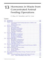
Simulation results of such a system show that this is essentially a two-state system
(Figure 13.1; parameter values in figure caption). For the first 3 days, the only particle
size class to change is that of single algal cells, which increases exponentially (lin-
ear in a logarithmic axis); larger particles have essentially constant concentrations.
With time, ever large particles have their concentrations changed. For the particles
composed of 30 monomers, there is an increase in concentration of about 10 orders
of magnitude between days 6 and 9. After day 9, there is essentially no change in
concentration. The difference in the first 3 days and the period after day 6 can be
understood as resulting from very few formation of aggregates at low algal concen-
trations, but formation of aggregates at a rate that matches algal division at higher
monomer concentrations. The rapid aggregate formation blocks any further increase
in algal numbers despite continued cell production.
The limitation can be understood by simplifying Equation (13.11) and assuming
that the most important loss for single cells is to collision and subsequent coagulation
Copyright 2005 by CRC Press
“L1615_C013” — 2004/11/18 — 22:33 — page 277 — #7
Models of Oceanic Plankton Aggregation 277
0
2
4
6
8
10
0
10
20

30
40
10
–10
10
–5
10
0
Time (day)Particle size (monomers)
Part concentration (# cm
–3
)
FIGURE 13.1 Number concentration of particles for an exponentially growing algal popu-
lation as a function of number of algal cells in a particle and time. The single algal cell with
a radius of r
1
= 10 µm and stickiness of α = 1 grows exponentially at µ = 1 per days in a
Z = 30 m thick mixed layer having a shear of γ = 1 sec
1
. Particle fall velocity is calculated
using a particle density of 1.036 g cm
−3
and fluid density of 1.0 g cm
−3
. The calculation uses
the summation formulation of Equations (13.11 and 13.12) and a rectilinear coagulation kernel.
with other single cells:
dC
1
dt

= µC
1
−αβ
11
C
2
1
(13.13)
where β
11
= 1.3γ(r
1
+r
1
)
3
(the rectilinear shear kernel). Note that the differential
sedimentation kernel for collisions between two particles of the same size is zero
because they fall atthe same rate, and that the Brownian kernel isconsiderably smaller
than thatfor shear for particles larger than 1 µm. At steadystate, the generationof new
algal cells by division balances the loss to coagulation. The resulting concentration
for the cells is
C
cr
=
µ
αβ
11
=
µ

1.3αγ 8r
3
1
(13.14)
Expressed as a volume concentration for spherical particles, this is:
C
V,cr
=
4
3
πr
3
1
µ
1.3αγ 8r
3
1
≈
πµ
αγ 8
(13.15)
Copyright 2005 by CRC Press
“L1615_C013” — 2004/11/18 — 22:33 — page 278 — #8
278 Flocculation in Natural and Engineered Environmental Systems
TABLE 13.2
Tests of Critical Concentration in Algal Blooms
Citation Test Result Comment
Kiørboe et al.
50
C

cr
for spring bloom Successfully
predict
maximum
concentration
Measure α
Riebesell
51,52
C
cr
for N. Sea bloom Prediction
10 ×high
Assume α = 0.1
Olesen
53
Maximum algal
concentration
Unclear. Chl
higher than
expected
No actual cell
concentration or
α measured
Prieto et al.
54
C
cr
in mesocosm Successful Conversion of
data required
Boyd et al.

55
C
cr
for Fe fertilization
experiment SOIREE
Successfully
predict non-
coagulation
Assume α = 1
Boyd et al.
55
C
cr
for Fe fertilization
experiment IronEx 2
Successfully
predict
timing of
export
Assume α = 1
Boyd et al. unpub-
lished results
C
cr
to Fe fertilization
experiment SERIES
Successfully
predict
maximum
concentration

Assume α = 1
The critical concentration provides a simple estimate of the maximum
concentration that algal population can attain during a bloom situation. It has been
remarkably successful when tested against bloom situations (Table 13.2). Its use
to predict the effect of ocean fertilization experiments is particularly striking.
55
The stickiness parameter α provides an important tuning parameter. Note that
Riebesell
51,52
would have successfully predicted the maximum bloom concentration
in the North Sea with α = 1 rather than the 0.1 he assumed.
13.3.1.2 Coagulation in a Stirred Container
One well-studied systemisa vessel with animposed(known)shear rate andaninitially
uniform (monodisperse) particle population.
56,57
In the initial stages of coagulation,
interactions among single particles dominate coagulation and, hence, the change
in total particle concentration C
T
. For small changes in particle number in C
1
, C
T
decreases by coagulation from collision of monomers:
dC
T
dt
=−
1
2

αβ
11
C
2
1
=−
1
2
α

4
3
γ(2r
1
)
3

C
2
1
=−
4αγ
π

4
3
πr
3
1
C

1

C
1
=−
4αγ
π
C
V,1
C
1
(13.16)
Copyright 2005 by CRC Press
“L1615_C013” — 2004/11/18 — 22:33 — page 279 — #9
Models of Oceanic Plankton Aggregation 279
0 0.05 0.1 0.15 0.2 0.25 0.3
200
300
400
500
600
700
800
900
1000
Time (days)
Total particle number concentration (# cm
–3
)
FIGURE 13.2 Total particle concentration through timefor an initiallymonodisperse system.

Solid line: solution calculated numerically using Equation (13.9); dashed line: approxim-
ate solution calculated using Equation (13.17). Calculation conditions: γ = 10 sec
−1
; r
1
=
10 µm; α = 1. Aggregate sizes in the calculation ranged from i = 1 to 100 monomers. There
was little lossof particle massfrom the system within the first 0.3days. Thedivergence between
the approximate and simulated solutions increases with decreasing particle numbers.
Further simplifying by assuming that C
V,1
is constant, the model predicts that
C
T
= C
0
exp

−
4αγ C
V,1
t
π

(13.17)
where C
0
is the initial particle concentration. The simplicity of this result has led to
its use to determine the value of α as a fitting parameter.
46,57,58

A numerical calculation of the coagulation in this system shows how the total
particle concentration changes in time (Figure 13.2). The rate of change does diverge
with time.
13.3.1.3 Steady-State Size Spectra
Hunt
8,9
applied the scaling techniques of Friedlander
20
to estimate the expected shape
of particle size spectra in aquatic systems. He predicted that the spectrum should be
proportional to the r
−2.5
, r
−4
, and r
−4.5
in the size ranges where Brownian motion,
shear, and differential sedimentation dominate. This calculation was based on a
scaling argument that assumes that particles are continually produced, that coagu-
lation moves mass to ever larger particles until they sediment out, and that only one
coagulation mechanism dominates at a given particle size.
Burd and Jackson
59
calculated the spectra numerically and compared them to the
results from scaling analysis (Table 13.3). Their results showed that the processes
Copyright 2005 by CRC Press
“L1615_C013” — 2004/11/18 — 22:33 — page 280 — #10
280 Flocculation in Natural and Engineered Environmental Systems
TABLE 13.3
Particle Size Spectral Slopes for Different Calculations

Brownian
Region
Shear
Region
Differential
Sedimentation
Region
Dimensional analysis −2.5 −4.0 −4.5
Numerical Base case −2.5 −5.0 −14.5
No settling −2.5 −6.3 −2.9
No settling, only 1 mech-
anism in size range
−2.5 −4.0 −4.6
Note: Thebasecase is anumericalsimulation using the sectionalapproach
with all coagulation mechanisms and particle settling possible for all
particles. The "no settling" cases result when there is no loss of particles
by settling out of a layer.
Source: From Burd and Jackson, Environ. Sci. Technol., 36, 323, 2002.
could not be considered separately. They were able to reproduce the scaling results
only when they omitted particlesettling and imposedonly one coagulationmechanism
in a given size range. Thus, the simple analysis is not necessarily correct.
13.3.2 RECTILINEAR AND HETERODISPERSE
Many of the simple relationships derived from coagulation theory implicitly assume
that the systems are initially monodisperse. It is made when assuming that particle
number is proportional to volume for all particles or, more basically, in the lineariza-
tions that are made to derive the simplified equations. The effect of the monodisperse
assumption can be tested by assuming that there are initially two particle sizes and
making similar simplifications.
13.3.2.1 Critical Concentration
The simplicity of the formulation and its lack of dependence on particle radius sug-

gest that it could be used to predict a critical concentration for mixed assemblages
of phytoplankton, where no one particle type dominates. An expanded version of
Equation (13.13) for two particles is
dC
a
dt
= µ
a
C
a
−αβ
aa
C
2
a
−αβ
ab
C
a
C
b
dC
b
dt
= µ
b
C
b
−αβ
bb

C
2
b
−αβ
ab
C
a
C
b
(13.18)
where the subscripts “a” and “b” are used to distinguish the two particles.
Copyright 2005 by CRC Press
“L1615_C013” — 2004/11/18 — 22:33 — page 281 — #11
Models of Oceanic Plankton Aggregation 281
At steady state, dC
a
/dt = 0 and the first part of Equation (13.18) reduces to
C
a
=
µ
a
αβ
aa
−
β
ab
C
b
β

aa
= C
a,cr
−
(r
a
+r
b
)
3
(r
a
+r
a
)
3
C
b
= C
a,cr
−
(r
a
/r
b
+1)
3
r
3
b

8r
3
a
C
b
= C
a,cr
−
(λ +1)
3
V
b
8V
a
C
b
where λ = r
a
/r
b
, V
a
=
4
3
πr
3
a
, and V
b

=
4
3
πr
3
b
. Expressing the concentrations in
terms of volumes and performing similar manipulations for C
b
yields:
C
Va
= C
V,cr
−
(1 +λ)
3
8
C
Vb
C
Vb
= C
V,cr
−
(1 +λ
−1
)
3
8

C
Va
(13.19)
where C
Va
= V
a
C
a
and C
Vb
= V
b
C
b
represent the volumetric concentrations of the
two particles, and C
V,cr
is the critical concentration for homogeneous distributions if
µ
a
= µ
b
(Equation 13.15). The problem is that if r
a
= r
b
, C
Va
and C

Vb
cannot both
be at steady state and have positive values: a larger particle is more likely to collide
with a smaller particle than vice versa. Thus, prediction for the simple monodisperse
system is not appropriate for the polydisperse system. It does, however, provide a
simple estimate.
13.3.2.2 Estimating Stickiness
The problem of using relationships derived for monodisperse systems to describe
the fate of heterodisperse systems extends to the method used to estimate
stickiness.
A modified version of Equation(13.16) todescribethe effectof collisions between
particles with two different sizes is then:
dC
T
dt
=−
1
2
αβ
aa
C
2
a
−
1
2
αβ
bb
C
2

b
−αβ
ab
C
a
C
b
=−
1
2
α

4
3
γ 8r
3
a
C
a
C
a
+
4
3
γ 8r
3
a
C
a
C

a

−α
4
3
γ(r
a
+r
b
)
3
C
a
C
b
=−
4αγ
π
(C
V,a
C
a
+C
V,b
C
b
) −
αγ
π


4
3
πr
3
b

(1 +λ)
3
C
a
C
b
=−
4αγ
π

C
V,a
C
a
+C
V,b
C
b
+
(1 +λ)
3
4
C
a

C
V,b

(13.20)
Copyright 2005 by CRC Press
“L1615_C013” — 2004/11/18 — 22:33 — page 282 — #12
282 Flocculation in Natural and Engineered Environmental Systems
where λ = r
a
/r
b
, C
V,a
= 4/3πr
3
a
C
a
, and C
V,b
= 4/3πr
3
b
C
b
. We would like to put
this into the form of Equation (13.16) in order to compare the heterodisperse and
monodisperse cases. Noting that the total volumetric concentration is related to the
volumetric concentrations of the components by
C

V,T
C
T
= (C
V,a
+C
V,b
)(C
a
+C
b
)
= C
V,a
C
a
+C
V,b
C
a
+C
V,a
C
b
+C
V,b
C
b
C
V,a

C
a
+C
V,b
C
b
= C
V,T
C
T
−C
V,b
C
a
−C
V,a
C
b
(13.21)
Substituting the results from Equation (13.21) into Equation (13.20) yields
dC
T
dt
=−
4αγ
π

C
V,T
C

T
−C
V,b
C
a
−C
V,a
C
b
+
(1 +λ)
3
4
C
a
C
V,b

=−
4γα
π
C
V,T
C
T

1 −
C
V,b
C

a
+C
V,a
C
b
−((1 +λ)
3
/4)C
a
C
V,b
C
V,T
C
T

=−
4γα
π
C
V,T
C
T

1 −
r
3
b
C
b

C
a
+r
3
a
C
a
C
b
−((1 +λ)
3
/4)C
a
r
3
b
C
b
r
3
a
C
2
a
+r
3
b
C
b
C

a
+r
3
a
C
a
C
b
+r
3
b
C
2
b

=−
4γα
π
C
V,T
C
T

1 −
1 +(r
a
/r
b
)
3

−((1 +λ)
3
/4)
(r
a
/r
b
)
3
(C
a
/C
b
) +1 + (r
a
/r
b
)
3
+(C
b
/C
a
)

=−
4γα

π
C

V,T
C
T
(13.22)
where α

= α(1 −
3
4
(1 − λ − λ
2
+ λ
3
)/(λ
3
η + λ
3
+ 1 + η
−1
)), η = C
a
/C
b
, and
λ = r
a
/r
b
. α


is the stickiness coefficient that would be estimated by using the
procedure for the monodisperse system. The value of α

depends on the relative sizes
and concentrations of the two particles (Figure 13.3).
13.3.3 C
URVILINEAR
Models of coagulation in planktonic systems have expanded in their use of both
ecological and coagulation descriptions. Recent models use moresophisticatedcoagu-
lation kernels, calculation schemes, fractal scaling on mass and ecological dynamics
(Table 13.4). The kernels in Equations (13.7) and (13.8) are used in the following
calculations.
13.3.3.1 Simple Algal Growth
The effect of changing the coagulation kernel on model results can be seen by
comparing the results from a simple model of exponential algal growth run with
Copyright 2005 by CRC Press
“L1615_C013” — 2004/11/18 — 22:33 — page 283 — #13
Models of Oceanic Plankton Aggregation 283
1 2 3 4 5 6 7 8 9 10
0.55
0.6
0.65
0.7
0.75
0.8
0.85
0.9
0.95
1
Ratio of radii, 

Estimated stickiness, Ј/
 =2
 =1
 = 0.5
FIGURE 13.3 Estimated stickiness α

relative to the actual stickiness α as a function of the
ratio of the radii λ for a polydisperse system. There are initially two distinct particles. Solid
line: η = 1; dashed line: η = 2; dash-dot: η = 0.5.
rectilinear and curvilinear kernels (Figure 13.4). These calculations use a sectional
approximation for the integral forms of the coagulation equations.
41
The results show
significant differences in steady-state particle concentrations (Figure 13.4a), timing
and magnitude of particle flux (Figure 13.4b), and average particle settling velocity
(Figure 13.4c).
The maximum particle concentration is higher for the curvilinear kernels than
for rectilinear, as should be expected from the more rapid rates of coagulation
(Figure 13.4). The steady-state concentrations of single algae for the rectilinear and
curvilinear kernels are 0.17 and 2.0 times the critical concentration calculated using
Equation (13.3) This higher value for the curvilinear kernel reflects the slower rates
of collision when using it.
Another difference is in the maximum total particle volumetric flux rate out
of the surface mixed layer, 49 and 488 cm
3
m
−2
per day for the rectilinear and
curvilinear kernels, respectively. This dramatic increase for the curvilinear calcu-
lation is a result of the larger particle concentrations available for removal when

the coagulation begins to dominate the growth. The peak average settling velo-
city is larger for the rectilinear kernel, 20 vs 12 m per day. The lower average
settling velocity is a reflection of the smaller average particle size in the curvi-
linear case.
The implication of this comparison is that the form of the coagulation kernel can
have a profound effectonpropertiesthat are ecologically significant, including particle
concentration and, even more dramatically, particle flux. Developers of models need
Copyright 2005 by CRC Press
“L1615_C013” — 2004/11/18 — 22:33 — page 284 — #14
284 Flocculation in Natural and Engineered Environmental Systems
TABLE 13.4
Features of Dynamic Models for the Marine Ecological Systems Involving
Coagulation
Citation Kernel Particle distribution M–L Scale Comments
Jackson
22
R Number of monomers O
Hill
24
C Sectional equivalent F Impose background
spectrum
Jackson and
Lochmann
23
C Sectional F
Riebesell and
Wolf-
Gladrow
60
C Number of monomers O

Jackson
47
C Sectional F Compare to expt
Ackleh and
Fitzpatrick
61
R Sectional equivalent V Explore math
properties
Ruiz
62
C O Diel turbulence
Mari and
Burd
63
C Sectional F TEP and phyto
Boehm and
Grant
64
R Jungian spectrum V
Kriest and
Evans
65
R 2-parameter spectrum V
Ackleh and
Forward
66
R Sectional equivalent V Adds self-shading
Jackson
44
P 2-D sectional F Multiple sources

Dadou et al.
67
E Two sizes O Vertical profile
Kriest
68
R 2-parameter spectrum V
Ruiz et al.
69
E 2 to 7 size classes — Fit expt results
Stemmann
et al.
70,71
P Sectional F Compare to midwater
observations
Note: Kernels: R — rectilinear; C — curvilinear; P — porous correction; E — empirical
fit; Mass–length (M–L) scale: V — volume conserved (m ∼ r
3
); F — fractal (m ∼ r
Df
);
O — other.
to discuss the implications of the formulations that they choose when publishing their
results.
13.3.3.2 Plankton Food Web Model
An example of the incorporation of coagulation into a more elaborate food web model
is the use of coagulation dynamics to describe the interactions of phytoplankton with
colloidal particles and fecal pellets in a food web model (as in Jackson
44
). By incor-
porating the multidimensional particle size spectra, the model includes aggregates

formed from the interaction of multiple particle types (Figure 13.5).
Copyright 2005 by CRC Press
“L1615_C013” — 2004/11/18 — 22:33 — page 285 — #15
Models of Oceanic Plankton Aggregation 285
10
–7
10
–6
10
–5
10
–4
Volume concentration (vol/vol)
(a)
Critical volume
Rectilinear
Rectilinear
Rectilinear
Curvilinear
Curvilinear
Curvilinear
0
100
200
300
400
Total flux (cm
3
m
–2

per day)
(b)
0 2 4 6 8 10 12 14 16 18 20
0
5
10
15
20
Time (days)
Average velocity (m per day)
(c)
FIGURE 13.4 Comparison of particle properties for a simple model with rectilinear and
curvilinear coagulation kernels. Calculations use a simple sectional model
55
for 50 m mixed
layer thickness, algal radius = 5 µm, specific growth rate µ = 0.5 per day, shear γ =
0.1 sec
−1
, and stickiness α = 1. Solid line indicates a rectilinear kernel; dashed line indicates
a curvilinear kernel. (a) Volumetric concentration. Lines with asterisks indicate total particle
concentrations; plain lines indicate the volumetric concentration of single algae; the critical
concentration isindicated with the dotted horizontal line. (b) Total particle flux at base of mixed
layer. (c) Average particle velocity = total flux/total particle concentration.
Copyright 2005 by CRC Press
“L1615_C013” — 2004/11/18 — 22:33 — page 286 — #16
286 Flocculation in Natural and Engineered Environmental Systems
10
–4
10
–3

10
–2
10
–1
10
–4
10
–3
10
–2
10
–1
10
–12
10
–10
10
–8
10
–6
10
–12
10
–10
10
–8
10
–6
Particle ∆ mass (g)
Particle ∆ mass (g)

Particle diameter (cm)
Particle diameter (cm)
0
0.1
0.2
0.3
0.4
0.5
0.6
0.7
Bin concentraton (M)
0
0.1
0.2
0.3
0.4
0.5
0.6
0.7
Bin flux (mmol m
–2
per day)
Colloid
Algal cell
Fecal pellet
Algal cell
Fecal pellet
Colloid
(a)
(b)

FIGURE 13.5 Results from a model incorporating two-dimensional particle size spectra,
fractal kernel, and a planktonic food web. This is similar to the model of Jackson
44
but for
conditions more typical of the North Atlantic. Concentrations and fluxes for “bins,” size ranges
whose upper masses are twice their lower and whose upper value of r
Df
are twice their lower.
(a) Concentration in each bin; (b) flux out of mixed layer for particles in the bin. There are
three particle sources: colloids, algae, and fecal pellets. The results are an example of using
multidimensional particle size spectra to incorporate multiple particle types.
Copyright 2005 by CRC Press
“L1615_C013” — 2004/11/18 — 22:33 — page 287 — #17
Models of Oceanic Plankton Aggregation 287
13.4 DISCUSSION
Simple coagulation models, such as those for the critical concentration and for
determining particle stickiness, have proven remarkably useful by providing simple
relationships that can be easily applied to interpret environmental data. Unfortunately,
the simple relationships do not work as well when applied to more realistic conditions
or accurate coagulation mechanisms.
72,73
As a result, the simple mechanisms should
be considered semi-quantitative at best.
The number of models of planktonic systems that incorporate coagulation is
surprisingly large (Table 13.4). Unfortunately, the range in their formulations is so
large that it is difficult to compare and interpret their results. Given the differences
resulting from different coagulation kernels, as illustrated above, it is difficult to
interpret them together. One response has been to abandon the theoretical structure
and instead use values for the interaction kernels determined by fitting results from
laboratory experiments.

69
While such an approach does fit the laboratory system,
it is unclear how to extrapolate the results to different environmental conditions.
Despite the importance that the choice of model formulation can have, there has been
remarkably little discussion or consensus on the best one to use.
Finding the best way to incorporate disaggregation into coagulation models for
marine systems remains an outstanding problem. There have been attempts to do
so,
34,62,74
but more needs to be done. Among the factors that need to be included
are the potential roles of zooplankton
75
and any other organisms
29
in weakening and
sundering marine aggregates.
One of the outstanding questions in aquatic systems is what is the precise role of
transparent exopolymeric particles (TEPs). These are organic particles that have been
associated with marine particle coagulation.
76–78
There have been several different
roles assigned to them: extra particles to participate in collisions,
63
agents for the
changing of particle stickiness,
79
and a separate system of coagulating particles.
76
Unfortunately for the resolution of the role of TEP on coagulation in natural waters,
most TEP studies have focused on the ecological aspects of the material and have not

accompanied them with the size spectral and stickiness measurements that could be
used to test the various possibilities. In future studies, measurements of particle size
spectra in conjunction with observations of TEP concentrations would make it easier
to test the role of TEP in coagulation.
Stemmann et al.
70,71
have developed a promising approach to test the importance
of coagulation, as well as biological processes, in determining particle distribu-
tions and fates. The method compares the particle size spectra measured through the
water column over time with those expected from different particle transformation
processes. This approach would be improved if there were a better quantitative under-
standing of how organisms, including bacteria and other microorganisms, change the
particle properties.
The particle size spectra are probably the most useful measurements that could be
made in systems where coagulation is believed to be important. Such measurements
should use multiple techniques in order to cover the range of important reactions.
34,35
In addition, multiple measurements on the same particles that could be used to test
models that invoke multidimensional particle size spectra would also help.
44,45
Copyright 2005 by CRC Press
“L1615_C013” — 2004/11/18 — 22:33 — page 288 — #18
288 Flocculation in Natural and Engineered Environmental Systems
13.5 CONCLUSIONS
The use of coagulation theory to describe particles in planktonic ecosystems is in a
transition phase. Simple models have provided simple, useable formulae to describe
marine systems. As the underlying models have been modified to improve the mech-
anistic descriptions, the simplicity is necessarily being left behind. Unfortunately,
there is no consensus on how the newer models should be formulated. Furthermore,
field observations tend to omit the collection of data that can be used to test the mod-

els. Progress in the field will depend on the ability of modeling and field programs to
interact.
ACKNOWLEDGMENTS
This chapter incorporates work with my various colleagues, including Steve Loch-
mann, Lars Stemmann, Thomas Kiørboe, and, most particularly, Adrian Burd. It has
been supported by grants, OCE-0097296 and OCE-998765, from the US National
Science Foundation.
REFERENCES
1. Sheldon, R.W., Prakash, A., and Sutcliffe, W.H., The size distribution of particles in
the ocean. Limnol. Oceanogr. 17, 327, 1972.
2. Gardner, W.D., Incomplete extraction of rapidly settling particlesfrom water samplers.
Limnol. Oceanogr. 22, 764, 1977.
3. Platt, T., and Denman, K., Organization in the pelagic ecosystem. Helgoland Wiss.
Meer. 30, 575, 1977.
4. Silvert, W., and Platt, T., Energy flux in the pelagic ecosystem: a time dependence
equation. Limnol. Oceanogr. 23, 813, 1978.
5. Rodriquez, J., and Mullin, M.M., Relation between biomass and body weight of
plankton in a steady state oceanic ecosystem. Limnol. Oceanogr. 31, 361, 1986.
6. Kiefer, D.A., and Berwald, J., A random encounter model for the microbial planktonic
community. Limnol. Oceanogr. 37, 457, 1992.
7. Zhou M., andHuntley, M.E., Populationdynamicstheoryofplanktonbasedon biomass
spectra. Mar. Ecol. Prog. Ser. 159, 61, 1997.
8. Hunt, J.R., Particle dynamics in seawater: implication for predicting the fate of
discharged particles. Environ. Sci. Technol. 16, 303, 1982.
9. Hunt, J.R., Prediction of oceanic particles size distributions from coagulation and
sedimentation mechanisms, in Particulates in water, Kavanaugh, M.C., and Leckie,
J.O., Eds., American Chemical Society, Washington, DC, p.243, 1980.
10. Trent, J.D., Shanks, A.L., and Silver, M.W., In situ and laboratory measurements
on macroscopic aggregates in Monterey Bay, California. Limnol. Oceanogr. 23, 626,
1978.

11. Kranck, K., and Milligan, T., Macroflocs: production of marine snow in the laboratory.
Mar. Ecol. Prog. Ser. 3, 19, 1980.
12. Kranck, K., and Milligan, T., Macroflocs from diatoms: in situ photography ofparticles
in Bedford Basin, Nova Scotia. Mar. Ecol. Prog. Ser. 4, 183, 1988.
13. Alldredge, A.L., and Silver, M.W., Characteristics, dynamics, and significance of
marine snow. Prog. Oceanogr. 20, 41, 1988.
Copyright 2005 by CRC Press
“L1615_C013” — 2004/11/18 — 22:33 — page 289 — #19
Models of Oceanic Plankton Aggregation 289
14. Alldredge, A.L., and Gotschalk, C., In situ settling behavior of marine snow. Limnol.
Oceanogr. 33, 339, 1988.
15. Logan, B.E., and Wilkinson, D.B., Fractal geometry of marine snow and other
biological aggregates. Limnol. Oceanogr. 35, 130, 1990.
16. O’Melia, C.R., An approach to modeling of lakes. Schweiz. Zeitsch. Hydrol. 34, 1,
1972.
17. Edzwald, J.K., Upchurch, J.B., and O’Melia, C.O., Coagulation in estuaries. Environ.
Sci. Technol. 8, 58, 1974.
18. O’Melia, C.R.,andBowman, K.S., Originsandeffects of coagulationinlakes. Schweiz.
Zeitsch. Hydrol. 46, 64, 1984.
19. Weilenmann, U., O’Melia, C.R., and Stumm, W., Particle transport in lakes: models
and measurement. Limnol. Oceanogr. 34, 1, 1989.
20. Friedlander, S.K., Smoke, dust and haze, Wiley, New York, 317 pp., 1977.
21. McCave, I., Size spectra and aggregation of suspended particles in the deep ocean.
Deep Sea Res. 31, 329, 1984.
22. Jackson, G.A., A model of the formation of marine algal flocs by physical coagulation
processes. Deep Sea Res. 37, 1197, 1990.
23. Jackson, G.A., and Lochmann, S.E., Effect of coagulation on nutrient and light
limitation of an algal bloom. Limnol. Oceanogr. 37, 77, 1992.
24. Hill, P., Reconciling aggregation theory with observed vertical fluxes following
phytoplankton blooms. J. Geophys. Res. 97, 2295, 1992.

25. Fenchel, T., Suspended bacteria as a food source, in Flows of energy and materi-
als in marine ecosystems, Fasham, M.J.R., Ed., Plenum Press, New York, p. 301,
1984.
26. Rothschild, B.J., and Osborn, T.R., Small-scale turbulence and plankton contact rates.
J. Plankton Res., 10, 465, 1988.
27. Shimeta, J., and Jumars, P.A., Physical mechanism and rates of particle capture by
suspension-feeders. Oceanogr. Mar. Biol. Ann. Rev. 29, 191, 1991.
28. Murray, A.G., and Jackson, G.A., Viral dynamics: a model of the effects of size, shape,
motion and abundance of single-celled planktonic organisms and other particles. Mar.
Ecol. Prog. Ser. 89, 103, 1992.
29. Kiørboe, T. Colonization of marine snow aggregates by invertebrate zooplankton:
abundance, scaling and possible role. Limnol. Oceanogr. 45, 479, 2000.
30. Kiørboe T., and Thygesen, U.H., Fluid motion and solute distribution around sinking
aggregates. II. Implications for remote detection by colonizing zooplankters. Mar.
Ecol. Prog. Ser. 211, 15, 2001.
31. Falconer, K.J., Fractal geometry: mathematical foundations and applications, Wiley,
New York, 1990.
32. Vicsek, T., Fractal growth phenomena, 2nd ed., World Scientific, NJ, 1992.
33. Li, X., and Logan, B.E., Size distributions and fractal properties of particles dur-
ing a simulated phytoplankton bloom in a mesocosm. Deep Sea Res. II, 42, 125,
1995.
34. Jackson, G.A., et al., Combining particle size spectra from a mesocosm experiment
measured usingphotographicandapertureimpedance(CoulterandElzone)techniques.
Deep Sea Res. II, 42, 139, 1995.
35. Jackson, G.A., et al. Particle size spectra between 1 µm and 1 cm at Monterey Bay
determined using multiple instruments. Deep Sea Res. I, 44, 1739, 1997.
36. Klips, J.R., Logan, B.E., and Alldredge, A.L., Fractal dimensions of marine
snow determined from image analysis of in situ photographs. Deep Sea Res. 41,
1159, 1994.
Copyright 2005 by CRC Press

“L1615_C013” — 2004/11/18 — 22:33 — page 290 — #20
290 Flocculation in Natural and Engineered Environmental Systems
37. Pruppacher, H.R., and Klett, J.D., Microphysics of clouds and precipitation, Reidel,
Boston, MA, 1980.
38. Adler, P.M., Streamlines in and around porous particles. J. Colloid Interface Sci. 81,
531, 1981.
39. Han, M., and Lawler, D.F., The (relative) insignificance of G in flocculation. J. Am.
Water Works Assoc. 84, 79, 1992.
40. Jackson, G.A., and Lochmann, S.E., Modeling coagulation in marine ecosystems, in
Environmental particles, volume 2, Buffle, J., and van Leeuwen, H.P., Eds., Lewis
Publishers, Boca Raton, FL, p. 387, 1993.
41. Gelbard, F., Tambour, Y., and Seinfeld, J.H., Sectional representations for simulating
aerosol dynamics. J. Colloid Interface Sci. 76, 541, 1980.
42. Li, X., and Logan, B.E., Collision frequencies of fractal particles with small particles
by differential sedimentation. Environ. Sci. Technol. 31, 1229, 1997.
43. Li, X., and Logan, B.E., Collision frequencies of fractal aggregates and small particles
in a turbulently sheared fluid. Environ. Sci. Technol. 31, 1237, 1997.
44. Jackson, G.A., Effect of coagulation on a model planktonic food web. Deep Sea Res.
I, 48, 95, 2001.
45. Jackson, G.A., Using fractal scaling and two dimensional particle size spectra to
calculate coagulation rates for heterogeneous systems. J. Colloid Interface Sci. 202,
20, 1998.
46. Kiørboe, T. Anderson, K., and Dam, H., Coagulation efficiency and aggregate
formation in marine phytoplankton. Mar. Biol. 107, 235, 1990.
47. Jackson, G.A., Comparing observed changes in particle size spectra with those
predicted using coagulation theory. Deep Sea Res. II 42, 159, 1995.
48. Alldredge, A.L., et al., The physical strength of marine show and its implications for
particle disaggregation in the ocean. Limnol. Oceanogr. 35, 1415, 1990.
49. Al-Ani, S., Dyer, K.R., and Huntley, D.A., Measurement of the influence of salinity
on floc density and strength. Geo-Marine Lett., 11, 154, 1991.

50. Kiørboe, T.P. et al., Aggregation and sedimentation processes during a spring phyto-
plankton bloom: a field experiment to test coagulation theory. J. Mar. Res. 52, 297,
1994.
51. Riebesell, U., Particle aggregation during a diatom bloom. I. Physical aspects. Mar.
Ecol. Prog. Ser. 69, 273, 1991.
52. Riebesell, U., Particle aggregation during a diatom bloom. II. Biological aspects. Mar.
Ecol. Prog. Ser. 69, 281, 1991.
53. Olesen, M., Sedimentation in Mariager Fjord, Denmark: the impact of sinking velocity
on system productivity. Ophelia 55, 11, 2001.
54. Prieto, L. et al., Scales and processes in the aggregation of diatom blooms: high time
resolution and wide size range records in a mesocosm study. Deep Sea Res. I, 49, 1233,
2002.
55. Boyd, P.W., Jackson, G.A., and Waite, A.M., Are mesoscale perturbation experiments
in polar waters prone to physical artefacts? Evidence from algal aggregation modelling
studies. Geophys. Res. Let. 29, 10.1029/2001GL014210, 2002.
56. Camp, T.R., and Stein, P.C., Velocity gradients and internal work in fluid motion.
J. Boston Soc. Civil Engrs. 30, 219, 1943.
57. Birkner, F.B., and Morgan, J.J., Polymer flocculation kinetics of dilute colloidal
suspensions. J. Am. Water Works Assoc. 60, 175, 1968.
58. Engel, A., The role of transparent exopolymer particles (TEP) in the increase in appar-
ent particle stickiness (α) during the decline of a diatom bloom. J. Plankton Res. 22,
485, 2000.
Copyright 2005 by CRC Press
“L1615_C013” — 2004/11/18 — 22:33 — page 291 — #21
Models of Oceanic Plankton Aggregation 291
59. Burd, A.B., and Jackson, G.A., Modeling steady state particle size spectra. Environ.
Sci. Technol. 36, 323, 2002.
60. Riebesell, U., and Wolf-Gladrow, D.F., The relationship between physical aggreg-
ation of phytoplankton and particle flux: a numerical model. Deep Sea Res. 39,
1085, 1992.

61. Ackleh, A.S., and Fitzpatrick, B.G., Modeling aggregation and growth processes
in an algal population model: analysis and computations. J. Math. Biol. 35,
480, 1997.
62. Ruiz, J., What generates daily cycles of marine snow? Deep Sea Res. I, 44,
1105, 1997.
63. Mari, X., and Burd, A., Seasonal size spectra of transparent exopolymeric particles
(TEP) in a coastal sea and comparison with those predicted using coagulation theory.
Mar. Ecol. Prog. Ser. 163, 63, 1998.
64. Boehm, A.B., and Grant, S.B., Influence of coagulation, sedimentation, grazing by
zooplankton on phytoplankton aggregate distributions in aquatic systems. J. Geophys.
Res. 103, 15601, 1998.
65. Kriest, I., and Evans, G., Representing phytoplankton aggregates in biogeochemical
models. Deep Sea Res. I 46, 1841, 1999.
66. Ackleh, A.S., and Forward, R.R., A nonlinear phytoplankton aggregation model with
light shading. SIAM J. Appl. Math. 60, 316, 1999.
67. Dadou, I. et al., An integrated biological pump model form the euphotic zone to the
sediment: a 1-D application in the Northeast tropical Atlantic. Deep Sea Res. II, 48,
2345, 2001.
68. Kriest, I., Differentparameterizationsofmarinesnowina1D-modelandtheirinfluence
on representation of marine snow, nitrogen budget and sedimentation. Deep Sea Res.
I, 49, 2133, 2002.
69. Ruiz, J., Prieto, L., and Ortegón, F., Diatom aggregate formation and fluxes: a model-
ing analysis under different size-resolution schemes and with empirically determined
aggregation kernels. Deep Sea Res. I, 49, 495, 2002.
70. Stemmann, L., Jackson, G.A., and Ianson, D., A vertical model of particle size dis-
tributions and fluxes in the midwater column that includes biological and physical
processes. I. Model formulation. Deep Sea Res. I, 51, 865, 2004.
71. Stemmann, L., Jackson, G.A., and Gorsky, G., A vertical model of particle size
distributions and fluxes in the midwater column that includes biological and physical
processes. II. Application to a three year survey in the NW Mediterranean Sea. Deep

Sea Res. I, 51, 885, 2004.
72. Farley, K.J., and Morel, F.M.M., Role of coagulation in the kinetics of sedimentation.
Environ. Sci. Technol. 20, 187, 1986.
73. Burd, A., and Jackson, G.A., The evolution of particle size spectra. I: pulsed input.
J. Geophys. Res. 102, 10545, 1997.
74. Hill, P.S., Sectional and discrete representations of floc breakage in agitated
suspensions. Deep Sea Res. I, 43, 679, 1996.
75. Dilling, L., and Alldredge, A.L., Fragmentation of marine snow by swimming macro-
zooplankton: a new process impacting carbon cycling in the sea. Deep Sea Res. I, 47,
1227, 2000.
76. Alldredge, A.L., Passow, U., and Logan, B.E., The abundance and significance of a
class of large, transparent organic particles in the ocean. Deep Sea Res. 40, 1131, 1993.
77. Passow, U., Transparent exopolymer particles (TEP) in aquatic environments. Prog.
Oceanogr. 55, 287, 2002.
Copyright 2005 by CRC Press
“L1615_C013” — 2004/11/18 — 22:33 — page 292 — #22
292 Flocculation in Natural and Engineered Environmental Systems
78. Logan, B.E., et al., Rapid formation and sedimentation of large aggregates is
predictable from coagulation rates (half-lives) of transparent exopolymer particles
(TEP). Deep Sea Res. II, 42, 203, 1995.
79. Kiørboe, T.P., and Hansen, J.L.S., Phytoplankton aggregate formation: observations of
patterns and mechanisms ofcellsticking and the significance of exopolymeric material.
J. Plankton Res. 15, 993, 1993.
Copyright 2005 by CRC Press