Structure and Function in Agroecosystem Design and Management - Chapter 12 ppt

CHAPTER 12
Impact of Grazing on
the Ecosystems
Daming Huang
CONTENTS
Introduction. . . . . . . . . . . . . . . . . . . . . . . . . . . . . . . . . . . . . . . . . . . . . . . . . . . . . 253
The Observational Site of an Alpine Meadow Grazing Ecosystem for a
Modeling Approach and Its Natural Conditions. . . . . . . . . . . . . . . . . . . 254
Modeling of an Alpine Meadow Grazing Ecosystem . . . . . . . . . . . . . . . . . . 255
Computer Program . . . . . . . . . . . . . . . . . . . . . . . . . . . . . . . . . . . . . . . . 261
Test of the Model . . . . . . . . . . . . . . . . . . . . . . . . . . . . . . . . . . . . . . . . . . 261
Sensitivity Analysis of Rotational Grazing Scheme . . . . . . . . . . . . . 261
A Simulated Rotational Grazing Experiment Using the Alpine
Meadow Grazing Ecosystem Model . . . . . . . . . . . . . . . . . . . . . . . . . . . . . 263
Maximum Potential Productivity of the Summer-Autumn Pasture
under Grazing. . . . . . . . . . . . . . . . . . . . . . . . . . . . . . . . . . . . . . . . . . . . . . . . 267
Maximum Potential Productivity of the SAP under
Grazing Pressure . . . . . . . . . . . . . . . . . . . . . . . . . . . . . . . . . . . . . . . . 267
Under Constant Grazing Pressure . . . . . . . . . . . . . . . . . . . . . . . . . . . . 269
Under Variable Grazing Pressure. . . . . . . . . . . . . . . . . . . . . . . . . . . . . 269
Discussion . . . . . . . . . . . . . . . . . . . . . . . . . . . . . . . . . . . . . . . . . . . . . . . . . . . . . . 271
Acknowledgments . . . . . . . . . . . . . . . . . . . . . . . . . . . . . . . . . . . . . . . . . . . . . . . 273
References . . . . . . . . . . . . . . . . . . . . . . . . . . . . . . . . . . . . . . . . . . . . . . . . . . . . . . 273
INTRODUCTION
The alpine meadow grazing ecosystem is a subsystem of the alpine
meadow ecosystem in QingZang Plateau, China. Grazing ecosystem research
253
0-8493-0904-2/01/$0.00+$.50
© 2001 by CRC Press LLC
920103_CRC20_0904_CH12 1/13/01 11:06 AM Page 253
has been conducted using an alpine meadow ecosystem matter cycling

energy flow biological complex modeling system approach since Shiyomi et
al. (1983). The meadow or pasture forms an ecosystem in which matter cycles
and energy flows through the constitutive components such as atmosphere,
plants, and animals, day by day. The amount of energy and materials passing
through or accumulating within these components is affected by factors in
complicated relations with each other. A grazing system embraces an entire
biological complex of weather, soil, plants, and animals, together with the
management imposed upon it by the grazier in order to attain desired objec-
tives, and it should be subject to evaluation by Shiyomi’s system approach
(1983, 1986). Modeling offers a way of bridging the gap between grazing
experiments and real grazing ecosystems, provided the model includes the
decision-making processes as well as the biological interactions between the
animals and the meadow. Efficient utilization of alpine meadow is one factor
of importance. The potential for highly efficient meadow husbandry opti-
mizing herd management can be evaluated by using modeling. From this
point of view, we are seeking, in the study, a rotational grazing scheme and
an optimal grazing pressure for the alpine meadow husbandry by modeling
an alpine meadow grazing ecosystem.
THE OBSERVATIONAL SITE OF AN ALPINE MEADOW
GRAZING ECOSYSTEM FOR A MODELING APPROACH AND
ITS NATURAL CONDITIONS
Alpine meadows cover vast areas of the QingZang (Tibet) Plateau, espe-
cially in the east and on high mountainous ranges. Amounting to 16 million
ha, alpine meadows cover 40% of the grassland in Qinghai Province. The
alpine meadow ecosystem research station, AFS, is located at Menyuan Stud
Ranch of Menyuan Hui Autonomous County, Haibei Tibetan Autonomous
Prefecture, Qinghai Province, 37°29Ј N-37°45Ј N and 101°12Ј E-101°33Ј E. The
station lies at the foothill on the south slope of Lenglongling Mountains in the
eastern part of the Qilian Mountains, in the northwest valley of the Datong
River. The lowest lands on the south side range between 3200 m and 3400 m

in altitude, forming a natural pasture where the station is situated. The high-
est peak of the Lenglongling Mountain range has an altitude of 5076 meters.
It is covered with snow all year, and the snow line is at about 4200 meters. The
Datong River valley does not vary much in topography and has an altitude
of 2800–3000 meters. In some places, the land has been farmed with rape
(Brassica campestris) as the main crop. Field surveys were carried out on the
experimental pastures of the AFS. There are 11 vegetation communities at the
AFS, of which the most important is a Kobresia humilis meadow. It is the most
common in the area of the AFS as well as on the Qinghai-Xizang Plateau and
is regarded as the best natural pasture. It is found on river banks, slopes, and
hills. The dominant species is Kobresia humilis, and subdominant species are
254 STRUCTURE AND FUNCTION IN AGROECOSYSTEMS DESIGN AND MANAGEMENT
920103_CRC20_0904_CH12 1/13/01 11:06 AM Page 254
Elymus nutans, Festuca ovina, Stipa aliena, etc., varying with the grazing pres-
sure. As to domestic animals, there are horses, yaks, and sheep. The AFS area
is grazed mainly by yaks and Tibetan sheep. The site parameters and pasture
conditions are summarized in Table 12.1.
MODELING OF AN ALPINE MEADOW GRAZING
ECOSYSTEM
In the alpine meadow pasture ecosystem, a portion of the solar energy is
fixed by pasture plants; some parts of these plants are grazed by grazing ani-
mals, and a fraction of the plants is fixed in animal bodies as energy. Energy
escaping from this fixation is accumulated as soil organic matter via feces and
urine, or diffused into the atmosphere from the animals as heat. Residual
plant matter changes into standing dead plant material and then into soil sur-
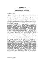
face litter, and finally accumulates in the soil. The system of energy flow in
the alpine meadow grazing ecosystem from sun to animals or soil is shown
in Fig. 12.1. In this figure, sources and sinks of energy are denoted by flags;
compartments in which energy accumulates temporarily are shown by rec-
tangles; directions of energy flow are indicated by arrow-heated full lines,

and influences, including environmental and artificial effects on the energy
flows which impinge upon the points shown by arrow-heated broken lines,
are denoted by ellipses. Bows indicated by arrow-headed broken lines denote
valves for regulating the energy flow. For example, the leaf area index or total
leaf area per given land area affects the amount of energy flowing from the
IMPACTS OF GRAZING ON THE ECOSYSTEMS 255
Table 12.1 Site Parameters and Experimental Pasture Conditions for
Modeling Approach
Item Explanation
Latitude 37°29ЈN-37°45ЈN
Longitude 101°12
ЈE-101°33ЈE.
Altitude 3100–3800m above sea level
Mean monthy air temperature minimum
Ϫ13°C (January), maximum 12.3°C
July), annual average 0°C
Mean monthly precipitation minimum 1.87 mm (January), maximum
114.7mm (July), annual total 531.6mm
Daily global solar radiation minimum 12558
kJ . m
Ϫ2
. day
Ϫ1
, maximum
21767.2
kJ . m
Ϫ2
. day
Ϫ1
, annual average

20930
kJ . m
Ϫ2
. day
Ϫ1
Pasture dominant plants Kobresia humilis, K. pygmaea, Stipa aliena,
Festuca ovina, Carex
spp., Poa spp., Elymus
nutans, Saussurea superba, Gentiana
straminea
Grazing conditions no fertilizer application; Tibetan sheep
920103_CRC20_0904_CH12 1/13/01 11:06 AM Page 255
sun to plants. That is, if this valve opens and the leaf area index becomes
larger, the amount of energy fixed in plants increases.
The amounts of energy accumulated in eight different compartments on
the grazing ecosystem are as follows: (1) above-ground live plant portion, V
1
,
(2) below-ground live portion including roots, V
2
, (3) underground dead por-
tion including roots, V
3
, (4) above-ground litter I (degradable portion includ-
ing sugar, starch, protein, animo acid, etc.), V
4
, (5) above-ground litter II
(undegradable portion including lignin, fat, tannin and wax), V
5
, (6) sheep

intake (pastural plants consumed by grazing animals), V
6
, (7) sheep
256 STRUCTURE AND FUNCTION IN AGROECOSYSTEMS DESIGN AND MANAGEMENT
Digestibility
Grazing
pressure:
S
Solar light
intensity:
A
Amount of
above-ground
live portion:
V
1
Leaf area
index:
L
Sun:
Q
0
Sheep liveweight:
V
7
Amount of sheep
intake:
V
6
Respiration:

Air-
temperature:
T
m
Amount of feces
+urine+methane:
V
8
Dead roots:
V
3
Live roots:
V
2
Soil:
Q
10
Amount of litter I:
Amount of
litter II:
V
5
V
4
Q
9
f
79
f
67

f
19
f
29
f
23
f
310
f
810
f
410
f
56
f
46
f
15
f
14
f
145
f
12
f
01
f
16
f
510

f
21
f
68
Figure 12.1 Energy flows of an alpine meadow grazing ecosystem.
920103_CRC20_0904_CH12 1/13/01 11:06 AM Page 256
liveweight, V
7
, (8) feces on the soil surface, V
8
. All these variables are meas-
ured in their calorific value and change with time t.
Changes in these variables can be formulated by a set of differential
equations as follow:
dV
1
/dt ϭ f
01
Q
0
ϩ f
21
V
2
Ϫ ( f
145
ϩ f
12
ϩ f
19

)V
1
Ϫ G
16
/S (12.1)
dV
2
/dt ϭ f
12
V
1
Ϫ ( f
21
ϩ f
23
ϩ f
29
)V
2
(12.2)
dV
3
/dt ϭ f
23
V
2
Ϫ f
39
V
3

(12.3)
dV
4
/dt ϭ f
14
f
145
V
1
Ϫ f
410
V
4
Ϫ G
46
/S (12.4)
dV
5
/dt ϭ f
15
f
145
V
1
Ϫ f
510
V
5
Ϫ G
56

/S (12.5)
dV
6
/dt ϭ (F
16
ϩ F
46
ϩ F
56
) Ϫ f
67
V
6
Ϫ f
68
V
6
(12.6)
dV
7
/dt ϭ D
D
ϫ C
O
/E
CV
(12.7)
dV
8
/dt ϭ f

68
V
6
/S Ϫ f
810
V
8
(12.8)
In Equations 12.1–12.8, the unit for these variables’ biomass (dry matter
17.752032 kJ/g, Daming et al, 1991), except V
6
and V
7
, is kJ/m
2
. The unit for V
6
is kJ sheep
Ϫ1
. day
Ϫ1
and for V
7
is kg/sheep. Parameters in Equations
12.1–12.8, f
ij
, denote energy flow rate from variable i to j, and they generally
change with the environmental temperature. The other parameters, G, S, etc.,
in the equations are explained in the following paragraphs. The main driving
variables are functions of time and expressed by following equations.

1. T
m
is the mean temperature during 1981–1985 (°C) (Daming et al.,
1991; Daming and Songling, 1992).
T
m
ϭ 1.11013 ϩ 0.153234 t Ϫ 6.5979 ϫ 10
Ϫ6
t
3
ϩ 4.004 ϫ
10
Ϫ13
t
6
Ϫ 7.9187 ϫ 10
Ϫ16
t
7
where t denotes the number of days counted from 21 April.
2. Global solar radiation on alpine meadow is expressed by a sine func-
tion as
Q
0
ϭ 17165.88 ϩ 4605.48 {sin [2
␲
(t ϩ 32)/365]} (kJ
.
m
Ϫ2

.
day
Ϫ1
)
The maximum and minimum values of Q
0
are 21771.36 and 12560.4 kJ .
m
Ϫ2
. day
Ϫ1
, respectively.
3. f
01
is the energy conversion efficiency of global solar radiation into
plant material (aboveground live plant portion), and it is expressed as
IMPACTS OF GRAZING ON THE ECOSYSTEMS 257
920103_CRC20_0904_CH12 1/13/01 11:06 AM Page 257
f
01
ϭ 95[1 Ϫ 1/(0.1019LV
1
)]A/(0.2388AQ
0
ϩ 1)
where L is the leaf area index and A is a constant which takes a value between
0 and 0.07.
A ϭ 0.035 ϩ 0.035 {sin[2
␲
(t ϩ 32)/365]}

L ϭ 3.238 ϫ 10
Ϫ4
ϩ 2.768 ϫ 10
Ϫ6
t ϩ 8.46 ϫ 10
Ϫ8
t
2
Ϫ 3.11 ϫ
10
Ϫ12
t
4
ϩ 1.519 ϫ 10
Ϫ19
t
7
4.f
i9
’s are coefficients of energy loss from the ith compartment, e.g., above-
ground plant portion, underground portion, etc., by respiration of plants
expressed as linear functions of air temperature (dimensionless).
5. f
i10
’s are coefficients of energy flow from the ith compartment, i.e., soil
surface litter or feces, to the soil, and they are functions of air temperature
(dimensionless). They and the other coefficients and parameters about pri-
mary production are listed in Table 12.2.
6. G
i6

(i ϭ 1,4,5. kJ . sheep
Ϫ1
. day
Ϫ1
) is the amount of herbage material
grazed by Tibetan sheep (Daming, 1993). The highest sheep food required is
F (kJ . sheep
Ϫ1
. day
Ϫ1
).
F ϭ 1725.872 ϫ V
7
0.75
The relationship between herbage intake, H
I
(kJ
.
sheep
Ϫ1
.
day
Ϫ1
), and
herbage allowance, A
L
, for sheep grazing on meadow is given by the follow-
ing equations (Daming, 1993):
H
I

ϭ
Ά
where A
L
ϭ (V
1
ϩ V
4
ϩ V
5
) ϫ S and S is the grazing area per sheep (m
2
/sheep).
The estimated critical value, M
D
, is
M
D
ϭ 1904.1 ϫ V
7
0.75
The amount of aboveground live plant portion, V
1
, grazed by sheep is
G
16
ϭ
Ά
The amount of aboveground litter I, V
4

, grazed by sheep is
G
46
ϭ
Ά
0 S ϫ V
1
Ն M
D
[V
4
/(V
4
ϩ V
5
)](1725.872 ϫ V
7
0.75
Ϫ G
16
) S ϫ V
1
Ͻ M
D
, A
L
Ն M
D
Ϫ0.9064 ϫ S ϫ V
4

A
L
Ͻ M
D
1725.872 ϫ V
7
0.75
S ϫ V
1
Ն M
D
0.9064 ϫ S ϫ V
1
S ϫ V
1
Ͻ M
D
0.9064 ϫ A
L
A
L
Յ M
D
F A
L
Ͼ M
D
258 STRUCTURE AND FUNCTION IN AGROECOSYSTEMS DESIGN AND MANAGEMENT
920103_CRC20_0904_CH12 1/13/01 11:06 AM Page 258
The amount of aboveground litter II, V

5
, grazed by sheep is
G
56
ϭ
Ά
So that F
16
ϭ G
16
/S, F
46
ϭ G
46
/S, F
56
ϭ G
56
/S and f
(145)6
ϭ f
16
ϩ f
46
ϩ f
56
7. f
68
is a proportion of feces, urine and methine energy in the herbage
grazed by sheep (Nanlin, 1982).

f
68
ϭ 0.490914
0 S ϫ V
1
Ն M
D
[V
5
/(V
4
ϩ V
5
)]/(1725.872 ϫ V
7
0.75
Ϫ G
16
) S ϫ V
1
Ͻ MD, A
L
Ն M
D
0.9064 ϫ S ϫ V
5
A
L
Ͻ M
D

IMPACTS OF GRAZING ON THE ECOSYSTEMS 259
Table 12.2 Parameters for Energy Flow Equations in the Primary Productivity
Compartment of the Model
Refs. 5, 3
f
12
ϭ
Ά
f
145
ϭ
Ά
f
14
ϭ 0.6 ϫ f
145
, f
15
ϭ 0.4 ϫ f
145
f
19
ϭ
Ά
f
21
ϭ
Ά
f
23

ϭ 6.738 ϫ 10
Ϫ4
f
29
ϭ
Ά
f
310
ϭ
Ά
f
410
ϭ
Ά
f
510
ϭ
Ά
3.153 ϫ 10
Ϫ5
T
m
ϩ 4.0033 ϫ 10
Ϫ3
(T
m
ՆϪ12.697)
0(
T
m

Ͻ Ϫ2.697)
1.9062
ϫ 10
Ϫ5
T
m
ϩ 2.4202 ϫ 10
Ϫ2
(T
m
ՆϪ12.697)
0(
T
m
Ͻ Ϫ12.697)
6.081
ϫ 10
Ϫ4
T
m
ϩ 1.56 ϫ 10
Ϫ3
(T
m
ՆϪ2.565)
0(
T
m
Ͻ Ϫ2.565)
5.5765

ϫ 10
Ϫ7
T
m
ϩ 21042 ϫ 10
Ϫ6
(T
m
ՆϪ3.373)
0(
T
m
Ͻ Ϫ3.373)
8.559
ϫ 10
Ϫ4
(t Յ 25)
0(
t Ͼ 25)
3.01 ϫ 10
Ϫ5
T
m
ϩ 1.139 ϫ 10
4
(T
m
ՆϪ3.784)
0(
T

m
Ͻ Ϫ3.784)
3.6237
ϫ 10
Ϫ4
(t Ͻ 133)
3.0703
ϫ 10
Ϫ2
(133 Ͻ t Ͻ 164)
0.5 (
t Ն 164)
0(
t Ͻ 101, t Ͼ 164)
2.6996
ϫ 10
Ϫ2
(101 Ͻ t Ͻ 164)
920103_CRC20_0904_CH12 1/13/01 11:06 AM Page 259
then
f
67
ϭ 1 Ϫ f
68
8. The relationship between the metabolic energy, M
E
, and V
6
is
M

E
ϭ f
67
ϫ V
6
The relationship between the rate of heat production as a multiple of basic
metabolism and the environmental temperature (Kleiber, 1961) is expressed as
Y ϭ
Ά
Then
D
mei
ϭ 293.076 ϫ Y ϫ V
7
0.75
where D
mei
represents the maintenance requirements of sheep, expressed in
grams of digestible organic matter per day.
9. When aboveground live biomass is below 2 t/ha, D
me
is increased to
account for greater energy spent in grazing such that (Huang, 1994):
D
me
ϭ D
mei
ϫ (1.8 Ϫ 0.4 ϫ C
TA
)

where
C
TA
ϭ (V
1
ϩ V
4
ϩ V
5
)/1775.2032 (t/ha)
10. Converse digestible organic matter intake to liveweight change. The
conversion function (E
CV
) is that derived by Arnold et al. (1977).
E
CV
ϭ (0.040 ϫ V
7
Ϫ 0.225)/0.54
Liveweight change (D
D
) is calculated in g/day as
D
D
ϭ (M
E
Ϫ D
mei
)/17752.032
ϭ [0.459 ϫ V

6
Ϫ 203.076 ϫ Y ϫ (1.8 Ϫ 0.6 ϫ C
TA
) ϫ V
7
0.75
/17752.032
and
C
o
ϭ
Ά
1 D
D
Ն 0
1.8
D
D
Ͻ 0
Ϫ0.05856 ϫ T
m
ϩ 2.167 T
m
Ͻ 13.125°C
1.3984 T
m
Ն 13.125°C
260 STRUCTURE AND FUNCTION IN AGROECOSYSTEMS DESIGN AND MANAGEMENT
920103_CRC20_0904_CH12 1/13/01 11:06 AM Page 260
Computer Program

The above process was written in BASIC as a program, Manager of
Alpine Meadow Grazing Ecosystems (MAMGE). The initial values of the
variables on 21 April (t ϭ 42) are given in Table 12.3. The constants and the
eight compartment values from which the program directly interpolates to
calculate and derive the value of the following function through integration
at each daily step: daily values and accumulated values of V
1
, V
2
, V
3
, V
4
, V
5
,
V
6
, V
7
, V
8
, Q
0
, Q
9
, Q
10
, T
m

, amount of biomass aboveground (V
1
ϩ V
4
ϩ V
5
),
amount of biomass underground (V
2
ϩ V
3
), etc.
Test of the Model
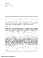
The predictions of the model were compared with experimental data
obtained from a cutting trial carried out at the AMERS, as shown in Figure
12.2(a). The modeling predicted the energy dynamics of the alpine meadow
grazing ecosystem as shown in Figure 12.2(b) for one year and in Figure
12.2(c) for four years. The calculated results fit the experimental data well.
The model was tested against experimental data from another rotation
grazing trial carried out at AMERS. Although the trial was not specifically
designed for this purpose, the conditions under which it was undertaken
seemed to be appropriate for comparison with the model output. The graz-
ing plan is described in Figure 12.3. Predicted and observed results of the
alpine meadow and sheep liveweight are shown in Table 12.4. The energy
dynamics of aboveground biomass in paddocks of the rotation grazing
experiment are shown in Figures 12.4a–e. The liveweight dynamics of sheep
in rotation grazing experiment are shown in Figures 12.4f and g.
Sensitivity Analysis of Rotational Grazing Scheme
Sensitivity analysis was applied to the model. The effects at 100 and 182
days of a 20% increase or decrease of the values of V

i
(i ϭ 1, 2, 3, 4, 5) are
shown in Table 12.5. The effects of a 20% increase or decrease temperature
(T
m
) or solar radiation (Q
0
) for 182 days are also shown in Table 12.5. The
results show that the system on 10 July (t ϭ 100 day) would be more stable
IMPACTS OF GRAZING ON THE ECOSYSTEMS 261
Table 12.3 Initial Values of the Variables on T ؍ 42 (21 April)
V
1t ϭ 42
ϭ 916.285 kJ . m
Ϫ2
V
6t ϭ 42
ϭ 0 kJ . m
Ϫ2
V
2t ϭ 42
ϭ 25534.238 kJ . m
Ϫ2
V
7t ϭ 42
ϭ 24.85 kg . sheep
Ϫ1
V
3t ϭ 42
ϭ 8128.224 kJ . m

Ϫ2
V
8t ϭ 42
ϭ 0 J . m
Ϫ2
V
4t ϭ 42
ϭ 15.266 kJ . m
Ϫ2
t
0
ϭ 42 (1 June)
V
5t ϭ 42
ϭ 271.382 kJ . m
Ϫ2
t
f
ϭ 182 (30 October)
920103_CRC20_0904_CH12 1/13/01 11:06 AM Page 261
262 STRUCTURE AND FUNCTION IN AGROECOSYSTEMS DESIGN AND MANAGEMENT
Below-ground biomass
Above-ground biomass
Plant dry weight (g/m
2
)
Month
(a)
4 5 6 7 8 9 10 11 12 1 2 3 4
2200

2000
1800
1600
400
200
0
Month
A
E
B
C
D
(b)
Biomass (x4.1868kj/m
2
)
7500
6500
5500
3000
2000
1000
0
4 5 6 7 8 9 10 11 12 1 2 3 4
Year
(c)
Biomass (x4.1868kj/m
2
)
A

F
B
C
D
E
1
234
7000
6000
5000
4000
2000
2000
1000
0
Figure 12.2 The simulation results of MAMGE (a) The aboveground biomass and
underground biomass of Kobresia humilis meadow. Solid line repre-
sents simulated values; Dotted line represents measured values. (b) For
one year. (c) For 4 years. A, live roots; B, dead roots; C, amount of above-
ground live portion (G
1
); D, litter I; E, litter II; F, amount of total above-
ground portion (G
1
ϩ G
4
ϩ G
5
).
920103_CRC20_0904_CH12 1/13/01 11:06 AM Page 262

than the system on 30 October (t ϭ 182 day), and that it is not disturbed eas-
ily by the environmental temperature and global solar energy.
A SIMULATED ROTATIONAL GRAZING EXPERIMENT USING
THE ALPINE MEADOW GRAZING ECOSYSTEM MODEL
A simulation experiment using MAMGE analyzed different rotational
grazing schemes for the common alpine meadow pastures at Qing-Zang
Plateau, China. The model is useful as a planning tool to enable subsequent
field research to focus on significant problems.
The simulated rotational grazing experiment included management
variables that reflect three options that can be chosen by a manager of rota-
tional grazing. One variable is the number of separate paddocks for rota-
tional grazing. Two to ten paddocks were included in this simulated
experiment. The second variable is the rotation period, which is the number
IMPACTS OF GRAZING ON THE ECOSYSTEMS 263
SA
4
SB
4
SC
4
SD
4
SE
4
2335.25 2796.75 3486.00 4625.75 6875.50
SA
3
SB
3
SC

3
SD
3
SE
3
2335.25 2796.75 3486.00 4625.75 6875.50
SA
2
SB
2
SC
2
SD
2
SE
2
2335.25 2796.75 3486.00 4625.75 6875.50
SA
1
SB
1
SC
1
SD
1
SE
1
2335.25 2796.75 3486.00 4625.75 6875.50
WA
3

WB
3
WC
3
WD
3
WE
3
3176.33 3804.33 4742.00 6292.33 9352.67
WA
2
WB
2
WC
2
WD
2
WE
2
3176.33 3804.33 4742.00 6292.33 9352.67
WA
1
WB
1
WC
1
WD
1
WE
1

3176.33 3804.33 4742.00 6292.33 9352.67
(a) 402.4m
200m
(a) 410.5m
200m
Figure 12.3 In a second rotational grazing trial, the meadow was divided into (a) a
summer-autumn pasture, SAP, (200 m ϫ 402.4 m) and (b) a winter-spring pasture,
WSP, (200 m ϫ 410.5 m). SA, SB, SE are the stock density classes. In the SAP, SA
1
,
SE
1
were grazed for 7 consecutive days, followed by SA
2
, SE
2
for 7 days, etc., return-
ing to SA
1
,SE
1
after a complete cycle of 28 days from 1 June to 30 October. In the
WSP, WA
1
, WE
1
were grazed for 10 consecutive days, followed by WA
2
,WE
2

for 10
days, etc., from November 1 to May 30, returning to WA
1
, WE
1
after 30 days. Every
paddock has ten sheep. The initial values of all variables are shown in Table 12.3.
920103_CRC20_0904_CH12 1/13/01 11:06 AM Page 263
264 STRUCTURE AND FUNCTION IN AGROECOSYSTEMS DESIGN AND MANAGEMENT
Table 12.4 Comparing Model Output (MD) with Observed Data (OD) in the Rotational Grazing Experiment
ABCDE
Date OD MD OD MD OD MD OD MD OD MD
Summer-autumn 31/05/1985 74.3 61.6 75.0 61.6 74.4 61.6 76.5 61.6 75.0 61.6
pasture (
g . m
Ϫ2
) 27/08/1985 265.0 115.2 253.6 152.9 249.0 186.8 262.4 217.7 254.7 246.6
02/11/1985 156.3 136.8 168.1 71.9 162.8 103.5 161.5 133.6 176.5 162.5
Winter-spring 31/05/1985 29.3 61.6 48.7 61.6 50.6 61.6 52.0 61.6 47.2 61.6
pasture (
g . m
Ϫ2
) 27/08/1985 242.4 300.8 245.1 300.8 258.8 300.8 258.0 300.8 249.8 300.8
02/11/1985 201.5 202.2 196.0 201.5 204.8 203.4 218.8 206.0 201.1 209.0
Tibetan sheep 31/05/1985 20.3 24.9 20.4 24.9 20.2 24.4 20.3 24.9 20.2 24.9
(kg . sheep
Ϫ1
) 31/10/1985 26.4 23.3 26.8 31.1 29.8 34.5 30.8 36.8 32.6 37.1
920103_CRC20_0904_CH12 1/13/01 11:06 AM Page 264
IMPACTS OF GRAZING ON THE ECOSYSTEMS 265

A
J
J
S
S
O
J
J
O
A
Sheep Liveweight
kg/sheep
f
g
80
60
40
20
0
4 5 6 7 8 9 10 11 12 4 5 6 7 8 9 10 11 1212 3 1 23
AAMJ J S SON D J J JFM ON DJFMMAA
E
A
B
C
D
A
B
C
D

E
1000
800
600
400
200
0
800
600
400
200
0
1000
800
600
400
200
0
1000
1200
Above-ground biomass
d
e
1
2
3
4
1
1
2

3
4
1
2
3
4
c
b
1
2
3
4
a
1
2
3
4
(V
1
+V
4
+V
5
)
(kj/m
2
)
Figure 12.4 The simulation results of a rotational grazing trial. a, b, c, d and e are the aboveground biomass (V
1
ϩ V

4
ϩ V
5
)
dynamics of SA
i
,SB
i
,SC
i
,SD
i
, and SE
i
(i ϭ 1, 2, 3, 4) paddocks under a given grazing pressure. The dotted line
shows the continuous grazing in SA, SB, SC, SD, and SE paddocks. The liveweight dynamics of Tibetan sheep
are shown in continuous grazing (f ) and rotational grazing (g) in SA, SB, SC, SD, and SE.
920103_CRC20_0904_CH12 1/13/01 11:06 AM Page 265
of consecutive days of grazing on each paddock. For example, if there are two
paddocks and the rotational period is three days, paddock 1 will be grazed
three consecutive days, followed by paddock 2 for three days, followed by
266 STRUCTURE AND FUNCTION IN AGROECOSYSTEMS DESIGN AND MANAGEMENT
Table 12.5 Sensitivity Analysis of Alpine Meadow Energy Dynamic System
Input disturbance Biomass Change Biomass Change
and parameter on 100 day rate on 182nd rate
disturbance (kJ . m
؊2
) (%) day (kJ . m
؊2
) (%)

V
1t ϭ 11
ϭ 248.36 4624.69 100 0.72 100
(
kJ . m
Ϫ2
)
V
2t ϭ 11
ϭ 26377.64 24528.78 100 30401.78 100
V
3t ϭ 11
ϭ 8792.55 6132.57 100 5416.86 100
V
4t ϭ 11
ϭ 40.72 15.01 100 1968.28 100
V
5t ϭ 11
ϭ 207.65 134.57 100 2367.91 100
V
1
5280.64 100 ϩ 14.18 0.76 10 ϩ 6.16
V
2
29434.52 100 ϩ 20.00 35757.13 100 ϩ 17.62
1.2
ϫ V
3
7359.08 100 ϩ 20.00 6478.01 100 ϩ 19.59
V

4
17.47 100 ϩ 16.38 2102.15 100 ϩ 6.80
V
5
160.96 100 ϩ 19.61 2546.14 100 ϩ 7.53
V
1
3911.11 100 Ϫ 15.43 0.66 100 Ϫ 7.44
V
2
19623.03 100 Ϫ 20.00 24926.08 100 Ϫ 17.95
0.8
ϫ V
3
4906.06 100 Ϫ 20.00 4352.41 100 Ϫ 19.65
V
4
12.42 100 Ϫ 17.24 1808.52 100 Ϫ 8.12
V
5
108.06 100 Ϫ 19.70 2159.20 100 Ϫ 8.81
4609.21 100
Ϫ 0.34 0.71 100 Ϫ 0.34
24526.87 100
Ϫ 0.01 30372.51 100 Ϫ 0.10
1.2
ϫ T
m
5675.55 100 Ϫ 7.44 4884.73 100 Ϫ 9.82
13.99 100

Ϫ 6.81 1937.49 100 Ϫ 1.56
129.26 100 Ϫ 3.95 2347.43 100 Ϫ 0.86
4640.22 100
ϩ 0.34 0.72 100 ϩ 0.33
24530.76 100
ϩ 0.09 30431.12 100 ϩ 0.10
0.8
ϫ T
m
6627.54 100 ϩ 8.07 6024.93 100 ϩ 11.23
16.20 100
ϩ 7.91 2000.20 100 ϩ 1.62
140.12 100 ϩ 4.12 2388.93 100 ϩ 0.89
4628.66 100
ϩ 0.09 0.72 100 ϩ 0.37
24528.78 100
ϩ 0.00 30410.19 100 ϩ 0.03
1.2
ϫ Q
0
6132.57 100 ϩ 0.00 5417.17 100 ϩ 0.00
15.02 100
ϩ 0.07 1971.81 100 ϩ 0.18
134.45 100 ϩ 0.01 2371.79 100 ϩ 0.16
4618.76 100
Ϫ 0.13 0.71 100 Ϫ 0.55
24528.78 100
Ϫ 0.00 30389.22 100 Ϫ 0.04
0.8
ϫ Q

0
6132.57 100 Ϫ 0.00 5416.47 100 Ϫ 0.01
15.00 100
Ϫ 0.10 1962.93 100 Ϫ 0.27
134.56 100 Ϫ 0.01 2362.10 100 Ϫ 0.25
920103_CRC20_0904_CH12 1/13/01 11:06 AM Page 266
paddock 1 for three days, etc. Thirty different rotation periods (from 1 to 30
days) were included in this simulation experiment. The third variable is the
simulated grazing pressure. Simulated grazing pressure refers to the amount
of dry biomass which is available for grazing. This variable is difficult to
study in actual grazing experiments because of variability in the grazing
intake among animals. However, the model can simulate different specified
grazing pressure by simulating different daily dry biomass grazed in kilo-
joules per m
2
; thus, the variability is avoided (Daming, 1994).
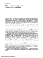
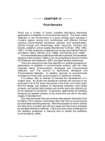
Two hundred and seventy different simulated grazing schemes (number
of paddocks ϫ rotational period ϭ 9 ϫ 30) were included in this experiment
(Figure 12.5). The critical grazing pressure of the alpine meadow is defined in
this paper as the event when simulated herbage growth does not provide
enough herbage biomass to allow for more grazing days (f
16
ϭ 0, f
46
ϭ 0,
f
46
ϭ 0). A summary of the accumulated dry biomass grazed is presented in
Figure 12.5. Thirty-five rotational grazing shemes produced significantly
higher accumulated dry biomass grazed (ϾJ

(145)
ϭ 3579.04 kJ/m
2
with
f
(145)6
ϭ 25.56 kJ . m
Ϫ2
.
day
Ϫ1
) than the other 235 schemes. The three most pro-
ductive specified rotation grazing schemes, three paddocks with a rotational
period of seven days, three paddocks with a rotation period of 29 days, and
four paddocks with a rotational period of 14 days produced high accumulated
dry matter grazed (Ͼ J
(145)
ϭ 4000 kJ/m
2
). The best one, three paddocks with a
rotational period of 7 days, had the highest accumulated dry biomass grazed
(J
(145)
ϭ 4250.44 kJ/m
2
with f
(145)6
ϭ 30.14 kJ . m
Ϫ2
. day

Ϫ1
). The results show that
the optimal paddock number of rotational grazing is three or four in an alpine
meadow grazing ecosystem. This is in accordance with Morley’s (1968) rec-
ommendation that the optimal paddock number should be below ten.
MAXIMUM POTENTIAL PRODUCTIVITY OF THE SUMMER-
AUTUMN PASTURE UNDER GRAZING
The potential productivity of the summer-autumn pasture (SAP) under
grazing is defined as the total herbage dry matter grazed by sheep over the
whole season (t ϭ 42 Ϫ 182 days). It has been analyzed by means of the opti-
mal control theory applied to compartment modeling of energy dynamics in
alpine meadow grazing ecosystem (Equations 12.1–12.5), with the produc-
tivity being regarded as an objective function to be maximized through opti-
mization under the following grazing pressures over the time.
Maximum Potential Productivity of the SAP under Grazing Pressure
Finding the maximum productivity of the SAP under constant grazing
pressure mathematically as
J
max
ϭ ͐
t
0
tf
(F
16
ϩ F
46
ϩ F
56
)dt

IMPACTS OF GRAZING ON THE ECOSYSTEMS 267
920103_CRC20_0904_CH12 1/13/01 11:06 AM Page 267
and the control constraint
0 Յ F
i6
Յ N(i ϭ 1, 4, 5) (N is the maximum reasonable value)
where F
16
ϭ G
16
/S, F
46
ϭ G
46
/S, F
56
ϭ G
56
/S. The values of initial state values
are: t
0
ϭ 42 (1 June), t
f
ϭ 182 (30 October), V
1tϭ42
ϭ 916.285 kJ/m
2
, V
2 t ϭ 42
ϭ

25534.238 kJ/m
2
, V
3 t ϭ 42
ϭ 8128.224 kJ/m
2
, V
4 t ϭ 42
ϭ 15.266 kJ/m
2
, V
5 t ϭ 42
ϭ
268 STRUCTURE AND FUNCTION IN AGROECOSYSTEMS DESIGN AND MANAGEMENT
GRAZING DURATION
FIELD NUMBER
ACCUMULATED INTAKE ( KJ/m
2
)
2951.69
3251.62 3551.56
3851.49
4151.42
26.00
21.00
16.00
11.00
6.00
1.00
2.0

6.0
10.0
Figure 12.5 The accumulated intake for 270 rotational grazing schemes under
critical grazing pressures.
920103_CRC20_0904_CH12 1/13/01 11:06 AM Page 268
271.382 kJ/m
2
. The results, given in Figure 12.6, were determined by the
Runge-Kutta method (Rao, 1984).
Under Constant Grazing Pressure
1. Suppose that V
1
Ն f
16
, f
16
ϭ c(cՆ 0 a constant), then if f
46
ϭ f
56
ϭ 0, we have
J
(1)
ϭ ͐
42
182
f
16
dt
J

(1) max
ϭ 3268.1777 kJ/m
2
(184.2248 g/m
2
)
while f
16
ϭ 25.8995 kJ . m
Ϫ2
. day
Ϫ1
(ϭ 1.4599 . m
Ϫ2
. day
Ϫ1
). The dynamics of
compartments are shown in Figures 12.6(a) and (c).
2. Suppose that f
16
ϭ c (c Ն 0 a constant), sometimes V
1
Ͻ f
16
then
f
46
ϭ ( f
16
Ϫ V

1
)V
4
/(V
4
ϩ V
5
)
f
56
ϭ ( f
16
Ϫ V
1
)V
5
/(V
4
ϩ V
5
)
and
J
(145)
ϭ ͐
42
182
( f
16
ϩ f

46
ϩ f
56
)t
The solution was obtained by the Runge-Kutta method with f
16
ϭ 0 ϳ 40, and
step ϭ 0.001.
J
(145) max
ϭ 3500.391 kJ/m
2
(197.316 g/m
2
)
while f
16
ϭ 25.92885 kJ . m
Ϫ2
. day
Ϫ1
(ϭ 1.4616 g . m
Ϫ2
. day
Ϫ1
). The dynamics of
every compartment are shown in Figures 12.5b–f.
Under Variable Grazing Pressure
The problem is
J

(145) max
ϭ ͐
42
182
( f
16
ϩ f
46
ϩ f
56
)t
The solution (Daming, 1994) is as follows.
The Hamilton is
H ϭ (f
16
ϩ f
46
ϩ f
56
) ϩ
␭
1
[ f
01
Q
0
ϩ f
21
V
2

Ϫ (f
145
ϩ f
12
ϩ f
16
)V
1
Ϫ f
16
]
ϩ
␭
2
[ f
12
V
1
Ϫ (f
12
ϩ f
23
ϩ f
26
)V
1
]
ϩ
␭
3

[ f
23
V
2
Ϫ f
37
V
3
]
ϩ
␭
4
[ f
14
f
145
V
1
Ϫ f
47
V
4
Ϫ f
46
]
ϩ
␭
5
[ f
15

f
145
V
1
Ϫ f
57
V
5
Ϫ f
46
]
IMPACTS OF GRAZING ON THE ECOSYSTEMS 269
920103_CRC20_0904_CH12 1/13/01 11:06 AM Page 269
270 STRUCTURE AND FUNCTION IN AGROECOSYSTEMS DESIGN AND MANAGEMENT
Figure 12.6 The potential productivity of the summer-autumn pasture (SAP) under constant grazing pressure. (a) ∑ 10.5∑G
1
and is the
relationship between grazing pressure and accumulated graze. (b) ∑10.5∑(G
1
ϩ G
4
ϩ G
5
). The maximum accumulated
graze. (c) J
(1)
.(d) J
(145)
.(e) The energy dynamics of aboveground biomass portion. (f ) The energy dynamics of under-
ground biomass portion.

920103_CRC20_0904_CH12 1/13/01 11:06 AM Page 270
where
␭
is Lagrangian multiplier. According to the Pontryagin maximum
principle,
f
i6
(i ϭ 1,4,5) ϭ
Ά
then
•
␭
1
ϭ Ϫ∂H/∂V
1
ϭ [ f
145
ϩ f
12
ϩ f
16
Ϫ ∂( f
01
Q
0
)/∂V
1
]
␭
1

•
␭
4
ϭ Ϫ∂H/∂V
4
ϭ f
47
␭
4
•
␭
5
ϭ Ϫ∂H/∂V
5
ϭ f
57
␭
5
We have
␭
1
ϭ
␭
4
ϭ
␭
5
ϭ 1
The necessary conditions for the existence of a singular are
f

16
ϭ f
01
Q
0
ϩ f
21
V
2
Ϫ 9.69AQ
0
LV
1
/[0.239AQ
0
ϩ 1)(1 ϩ 0.102LV
1
)
2
] Ϫ dV
1
/dt (12.9)
f
46
ϭ f
14
f
145
V
1

Ϫ dV
4
/dt (12.10)
f
56
ϭ f
15
f
145
V
1
Ϫ dV
5
/dt (12.11)
Computing of modeling systems provided an inference base to support a rec-
ommendation concerning the grazing pressure and accumulated intake. The
recommendation is as follows: under constant grazing pressure, the subopti-
mal grazing pressure is 25.90 J . m
Ϫ2
. day
Ϫ1
with a higher accumulated intake
J
(1)
ϭ 3268.17 kJ/m
2
, and the optimal grazing pressure is 25.94 J . m
Ϫ2
. day
Ϫ1

with the maximal accumulated intake J
(145)
ϭ 3500.39 kJ/m
2
. Under variable
grazing pressure, the dynamics of optimal grazing pressure are shown in
Figures 12.7a–d and Equations 12.9–12.11, while the highest accumulated
grazing is J
(145)
ϭ 8749.01 kJ/m
2
, 2.5 times the optimal under constant grazing
pressure.
DISCUSSION
Should a pasture be grazed continuously at a uniform stock density, or
should it be divided into subplots to be grazed in turn by the whole herd in
a rotational manner, so each subplot receives alternate periods of heavier
grazing and of rest? Should there be many or few subplots, and should the
rotation cycle be long or short? These questions have for long been contro-
versial among both pastoralists and scientists. Although all the theoretical
0 as
␭
Ͼ 1
undefined as
␭
ϭ 1
N as
␭
Ͻ 1
IMPACTS OF GRAZING ON THE ECOSYSTEMS 271

920103_CRC20_0904_CH12 1/13/01 11:06 AM Page 271
questions seem to be solved by creative research (Noy-Meir, 1976) using a
simple mathematical model which represents only the minimum essential
features of the major processes involved, actual questions from concrete pas-
tures should be solved by more explicit models, ecosystem modeling, or
expert systems.
The productivity of the alpine meadow grazing ecosystem is also
strongly affected by climate and soil conditions which are almost uncontrol-
lable (Coupland, 1979). Our research purpose for the alpine meadow grazing
ecosystem is to raise primary and secondary production under conditions of
sustainable development. It has been shown in this paper that if we manage
pasture more effectively, higher plant and animal production can be obtain-
able. Considering the dearth of information based on which the model is
built, it is concluded that the model gives encouragingly accurate predictions
of grass growth and liveweight changes in the alpine meadow grazing
meadow. Given a broader data base on initial values in different situations,
the model could be used by advisers to help farmers in similar environments
and to decide the strategies for using their alpine meadows. Output of the
272 STRUCTURE AND FUNCTION IN AGROECOSYSTEMS DESIGN AND MANAGEMENT
Below-ground biomass (kj/m
2
)
Maximum accumulated intake
(kj/m
2
)
Optimum variable grazing
pressure (kjm
-2
day

-1
)
Above-ground biomass (kj/m
2
)
1600
800
0
0
0
8000
8000
4000
4000
40000
20000
0
42 82 122 162 182
42 82 122 162 182
Time (day) Time (day)
(a)
(b)
(c)
(d)
V
2
J
(1)
J
(4)

J
(5)
V
4
V
1
V
5
V
3
f
16
f
46
f
56
Figure 12.7 The potential productivity of the summer-autumn pasture (SAP) under
variable grazing pressure. (a) The optimum variable grazing pressure.
(b) The maximum accumulated graze. (c) The energy dynamics of
aboveground biomass portion. (d) The energy dynamics of under-
ground biomass portion.
920103_CRC20_0904_CH12 1/13/01 11:06 AM Page 272
model will be used to develop a system of field experiments to study grazing
measurement. This procedure can make effective use of limited financial
resources to obtain information that is relevant to pasture management.
ACKNOWLEDGMENTS
Financial assistance from the DAAD/K.C.Wong Foundation of Germany
for this research is hereby acknowledged. The authors also acknowledge the
contributions of Mrs. Steinbach, Dr. Tony Goodchild (Reading University,
U.K.) and Professor Mase Shiyomi. Thanks are also due to the anonymous

referees for their comments.
REFERENCES
1. Arnold, G.W., Campbell, N.A. and Galbraith, K.A. Mathematical relationships
and computer routines for a model of food intake, liveweight change and wood
production in grazing sheep.
Agric. Sys., 1977, 2:209–226.
2. Coupland, R.T.
Grassland Ecosystems of the World. Cambridge University Press,
London, 1979.
3. Huang, D. Compartment modeling of an alpine meadow grazing ecosystem.
Journal of Xiamen University (Natural Science), 1993, 32(6):768–772.
4. Huang, D., Zuwang, W., Nanlin, P. and Li, Z. A study of energy flow and eco-
nomic value of a family pasture in an alpine pastoral area.
Alpine Meadow Ecosys.,
1991, 3:381–402.
5. Huang, D. and Songling, Zhao. Compartment modeling of energy dynamics in
Kobresia humilis meadow. Acta Ecologia. Sinica, 1992, 12(2):119–124.
6. Huang, D. Systematic analysis of rotation grazing experiment in alpine meadow
ecosystem.
J. Xiamen University (Natural Science), 1994, 33(2):259–264.
7. Kleiber, M. The fire of life: an introduction to animal energetics. John Wiley &
Sons, New York, 1961.
8. Morley, F.H.W. Aust.
J. Exp. Agric. Anim. Husb., 1968, 8:40–45.
9. Nanlin, P. Energy dynamics of the sheep population in alpine meadow ecosystem:
I. measurement of the daily food grazing, feces and urine of Tibetan sheep.
Alpine
Meadow Ecosys.,
1982, 1:67–72.
10. Noy-Meir, I. Rotational grazing in a continuously growing pasture: a simple

model.
Agric. Sys., 1976, 10:87–112.
11. Orsini, J.P.G. and Arnold, G.W. Predicting the liveweight change of sheep grazing
wheat stubbles in a Mediterranean environment.
Agric. Sys., 1986, 20:83–103.
12. Rao, S.S.
Optimization, theory and applications. 2nd ed. Wiley Eastern Limited, 1984.
13. Shiyomi, M., Takahashi, S., Akiyama, T., Hirosaki, S. and Okubo, T. A preliminary
simulation model of grazing nature ecosystem.
Bull. Nat. Grassl. Res. Inst., 1983,
22:27–43.
14. Shiyomi, M., Akiyama, T. and Takahashi, S. Modeling of energy flows and con-
version efficiencies in a grassland ecosystem.
Ecol. Modeling, 1986, 32:119–135.
15. Shiyomi, M. and Takahashi, S. A formulation of the relationship between herbage
allowance and herbage intake for animals on grazed pasture.
J. Japn. Soc.
Grassland Sci.,
1987, 32(4):299–306.
IMPACTS OF GRAZING ON THE ECOSYSTEMS 273
920103_CRC20_0904_CH12 1/13/01 11:06 AM Page 273