Particles in Water Properties and Processes - Chpater 4 doc
Bạn đang xem bản rút gọn của tài liệu. Xem và tải ngay bản đầy đủ của tài liệu tại đây (1.4 MB, 30 trang )
63
chapter four
Colloid interactions and
colloid stability
4.1 Colloid interactions — general concepts
Between particles in water there are various kinds of interaction, depending
on the properties, especially surface properties, of the particles. These inter-
actions can give forces of attraction or repulsion. If attractive forces dominate,
then the particles will stick together on contact and form clusters or
aggre-
gates.
When particles repel each other they are kept apart and prevented
from aggregating. In the latter case, the particles are said to be
stable,
whereas
when aggregates can form, the particles are
unstable
or
destabilized.
Because
these concepts are mainly relevant to particles in the colloidal size range,
the subject is known as
colloid stability
and the interactions are known as
colloid interactions.
These topics are dealt with in this chapter.
4.1.1 Importance of particle size
Before dealing with the different types of colloid interactions, it is worth
pointing out some important general features. The first point is that colloid
interactions are usually of rather short range — usually much less than the
particle size. Thus, they do not come into play until particles are nearly in
contact and so do not have much influence on the transport of particles,
which is still governed by mechanisms discussed in Chapter 2 (i.e., diffusion,
sedimentation, and convection). When particles
do
approach very close, then
colloid interactions are crucial in determining whether attachment occurs.
The other important feature is the dependence of the interactions on
particle size. As we shall see, in most cases, the strength of interaction is
roughly proportional to the
first power
of the particle size. There are other
important forces acting on particles, which were discussed in Chapter 2 (i.e.,
fluid drag and gravitational attraction). Fluid drag is proportional to the
projected area of the particle and thus roughly to the
square
of the particle
size. The gravitational force is proportional to the mass of the particle and
hence to the
cube
of particle size.
TX854_C004.fm Page 63 Wednesday, August 3, 2005 10:48 AM
© 2006 by Taylor & Francis Group, LLC
64 Particles in Water: Properties and Processes
These different size dependences are of enormous significance because
they mean that colloid interactions become less important as particle size
increases. This is illustrated schematically in Figure 4.1. Here two spherical
particles are in contact with a flat wall and are subject to three different forces:
• An attractive force,
F
A
, holding the particles to the wall
• Fluid drag,
F
D
, caused by flow parallel to the surface
• Gravitational attraction,
F
G
, acting vertically downward, opposite to
F
A
.
The two particles have diameters that differ by a factor of two, and the
magnitude of the forces is indicated by the lengths of the arrows. For the
smaller particle, the attractive force is greater than the gravitational force
and hence the particle remains attached. However, for the larger particle,
although
F
A
is doubled,
F
G
is greater by a factor of 8 than for the smaller
one. This means that gravity would be sufficient to detach the larger particle.
The drag force is increased by a factor of 4, and this may also play a part in
detaching the larger particle. This simple example provides an explanation
for the common observation that colloid interactions are much more signif-
icant for smaller particles and that larger particles can more easily be
detached by fluid drag or other external forces, such as gravity. This is the
main reason why the effects are known as
colloid
interactions.
4.1.2 Force and potential energy
The various types of colloid interaction give rise to
forces
between particles,
which can be directly measured in some cases. However, it is often conve-
nient to think in terms of a
potential energy
of interacting particles. These
Figure 4.1
Forces on a sphere close to a flat plate. F
A
: Attractive colloid force (such
as van der Waals attraction); F
D
: Fluid drag; F
G
: Gravitational attraction. For the
smaller particle (
left)
the colloid force is largest, but for the larger particle the other
forces are relatively more significant.
F
A
F
D
F
G
TX854_C004.fm Page 64 Wednesday, August 3, 2005 10:48 AM
© 2006 by Taylor & Francis Group, LLC
Chapter four: Colloid interactions and colloid stability 65
two concepts can be related simply by considering the work involved in
bringing the particles from a large (effectively infinite) distance, where the
interaction is negligible, to a given separation
h.
This gives the energy of
interaction. If the interaction force at a separation distance
x
is
P(x)
, then the
work done in moving through a distance
δ
x
is
P(x)
δ
x.
Thus, the total work
done in bringing the particles to a separation
h,
or the potential energy of
interaction,
V,
is as follows:
(4.1)
Conventionally the sign of the force is positive for repulsion and negative
for attraction, and the same applies to the energy of interaction.
It is usually easier to derive the interaction force, and then the corre-
sponding energy can be calculated using Equation (4.1).
4.1.3 Geometry of interacting systems
A common method of approaching the problem of interaction between par-
ticles is to first derive the interaction between parallel flat plates as a function
of separation distance. Some aquatic particles
are
platelike in character (e.g.,
clays), but in many cases we need to consider the interaction of particles that
are roughly spherical in shape. It is possible to derive approximate expres-
sions for interaction of spherical particles (and other shapes) by a method
developed by Deryagin in 1934. We shall consider only two cases: the inter-
action of unequal spheres and between a sphere and a flat surface. Both of
these are relevant to many common problems involving colloid interactions
and are illustrated in Figure 4.2, together with the parallel plate case.
Figure 4.2
Showing interactions between (a) parallel flat plates, (b) unequal spheres,
and (c) a sphere and a plate. In all cases the separation distance is
h.
VPxdx
h
=
∞
∫
()
h
d
1
h
d
2
d
1
h
(a) (b) (c)
TX854_C004.fm Page 65 Wednesday, August 3, 2005 10:48 AM
© 2006 by Taylor & Francis Group, LLC
66 Particles in Water: Properties and Processes
The Deryagin approach makes the assumption that the interaction
between spheres can be treated as the sum of interactions between concentric
parallel rings, instead of the actual sphere surfaces. This approximation is
only valid when the separation distance is much less than the sphere diam-
eter. However, because colloid interactions are usually of small range, this
is not often a serious limitation. If the
energy
of interaction per unit area of
parallel plates, separated by a distance
h,
is
V(h),
then the interaction
force
between unequal spheres, diameters
d
1
and
d
2
, turns out to be simply:
(sphere–sphere) (4.2)
For the case of a sphere interacting with a flat plate, the force can be
derived simply from the sphere–sphere case by letting one sphere become
very large (
d
2
=
∞
):
(sphere-plate) (4.3)
(This is just twice the force between two equal spheres of diameter
d
1
, at a
distance
h)
.
If the energy of interaction is needed, rather than the force, then Equation
(4.1) can be used, with the appropriate force expression. It must be remem-
bered that Equations (4.2) and (4.3) are only appropriate for very small
separation distances (
h << d
1
). They become inaccurate for larger distances.
4.1.4 Types of interaction
The following types of colloid interaction are important in practice and will
be discussed in subsequent sections:
• van der Waals (usually attractive)
• Electrical double layer (either repulsive or attractive)
• Hydration effects (repulsive)
• Hydrophobic (attractive)
• Steric interaction of adsorbed layers (usually repulsive)
• Polymer bridging (attractive)
The first two of these interactions (van der Waals and electrical double
layer) form the basis of a quantitative theory of colloid stability developed
around 1940 by Deryagin and Landau and, independently, by Verwey and
Overbeek. In recognition of these pioneers, the theory is now widely known
as
DLVO theory.
The remaining interactions are not taken into account in the
theory; these are sometimes called
non-DLVO forces.
Ph
dd
dd
Vh() ()=
+
π
12
12
Ph dVh() ()=π
1
TX854_C004.fm Page 66 Wednesday, August 3, 2005 10:48 AM
© 2006 by Taylor & Francis Group, LLC
Chapter four: Colloid interactions and colloid stability 67
These interactions and their effects on colloid stability will be considered
in the following sections.
4.2 van der Waals interaction
4.2.1 Intermolecular forces
Between all atoms and molecules there are attractive forces of various kinds,
which J.D. van der Waals postulated in 1873 to account for the nonideal
behavior of real gases. If the molecules are polar (i.e., with an uneven dis-
tribution of charge), then attraction between dipoles is important. When only
one of the interacting molecules has a permanent dipole, then it can induce
an opposite dipole in a nearby molecule, thus giving an attraction. Even
when the atoms or molecules are nonpolar, the movement of electrons
around nuclei give “fluctuating dipoles,” which induce dipoles in other
molecules and hence an attraction. From the standpoint of colloid stability
this is the most important of the intermolecular interactions. It is a quan-
tum-mechanical effect, first recognized by Fritz London in 1930. For this
reason the resulting forces are sometimes known as
London-van der Waals
forces.
However they are also known as
dispersion forces
because the funda-
mental electron oscillations involved are also responsible for the dispersion
of light. (This term may be a source of some confusion — it does not refer
to dispersions of particles.)
All of these interactions show the same distance dependence — the
energy of attraction between molecules varies inversely as the
sixth
power
of separation distance,
r
:
(4.4)
where
B
is a constant that depends on the properties of the interacting
molecules (often known as the
London constant)
and the negative sign indi-
cates an attraction.
The dependence on
1/r
6
shows that the interaction falls off rapidly with
increasing distance. However, between macroscopic objects, the attraction is
of longer range and plays a vital part in the interaction of colloidal particles.
4.2.2 Interaction between macroscopic objects
All objects are assemblies of atoms and molecules, subject to the intermo-
lecular interactions just discussed. In principle, the total interaction between
two objects, of known geometric form, can be derived by adding up all of
the individual intermolecular attractions. The summation is replaced by
integration over the volumes of the interacting objects, and the result
depends on the number of molecules per unit volume and the appropriate
Vr
B
r
()=−
6
TX854_C004.fm Page 67 Wednesday, August 3, 2005 10:48 AM
© 2006 by Taylor & Francis Group, LLC
68 Particles in Water: Properties and Processes
London constant,
B.
Such an approach was adopted by H.C. Hamaker in the
1930s; he showed that the resulting interactions could be appreciable at large
separations. Some results are given below.
For
two parallel flat plates
separated by a distance
h,
the van der Waals
energy of attraction per unit area is found to be the following:
(4.5)
This expression is based on the assumption that the plates are “infinitely
thick.” (In practice this means that the thickness should be much greater
than the separation distance.) The equation applies to the case where the
two plates are composed of different materials, 1 and 2. The constant
A
12
is
known as the
Hamaker constant,
which depends on the properties of the two
materials. It is given by the following:
(4.6)
where
N
1
and
N
2
are the numbers of molecules per unit volume in the two
materials and
B
12
is the London constant for the interaction of molecules 1
and 2.
Hamaker constants will be discussed further in the next section.
For the interaction of
unequal spheres,
the Hamaker expression is as
follows:
(4.7)
where x = h/d
1
and y = d
2
/d
1.
For the sphere-flat plate case, the second sphere is assumed to be infi-
nitely large (y =
∞
), and the interaction energy becomes the following:
(4.8)
These expressions can be considerably simplified if it is assumed that
the separation distance is very small (
x
<<
1
)
. This gives
(sphere–sphere) (4.9)
V
A
h
A
=−
12
2
12π
ANNB
12
2
1212
=π
V
Ay
xxyx
y
xxyxy
xxyx
xx
A
=−
++
+
+++
+
++
+
12
22
2
2
12
2ln
yyxy++
⎡
⎣
⎢
⎤
⎦
⎥
V
A
xx
x
x
A
=− +
+
+
+
⎡
⎣
⎢
⎤
⎦
⎥
12
12
11
1
2
1
ln
V
A
h
dd
dd
A
=−
+
12 1 2
12
12 ( )
TX854_C004.fm Page 68 Wednesday, August 3, 2005 10:48 AM
© 2006 by Taylor & Francis Group, LLC
Chapter four: Colloid interactions and colloid stability 69
(sphere-plate) (4.10)
These short-range expressions can also be derived by applying the Dery-
agin method, Equations (4.2) and (4.3), using the flat-plate energy expression,
Equation (4.5). This gives expressions for the force, which, when integrated
according to Equation (4.1), yield the same results as Equations (4.9) and
(4.10). These are not good approximations when the separation distance
exceeds a few percent of the particle diameter. Figure 4.3 shows calculated
values of the interaction energy for two equal spheres as a function of
dimensionless separation distance
h/d.
The energy is also expressed in
dimensionless form, as a ratio with the Hamaker constant,
V/A.
Although
not very accurate, the short-range expressions are adequate for many prac-
tical purposes.
It is clear that the van der Waals attraction between macroscopic objects
has a different dependence on distance than that between molecules. The
flat-plate energy depends inversely on the square of the separation distance,
and for spheres at close approach there is a 1/
d
dependence. This means
that the interaction falls much more slowly with increasing distance than
the 1/
r
6
behavior for a pair of molecules. For this reason, van der Waals
interaction is much more significant for particles than was originally thought.
It is also clear from the short-range expressions for spheres that the
energy is directly proportional to the sphere diameter. Although, in general,
Figure 4.3
Comparison of van der Waals attraction between equal spheres, calculated
from the complete Hamaker expression, Equation (4.7), and the approximate,
short-range expression, Equation (4.9).
1E−3 0.01 0.1 1
0.1
1
10
100
eq (4.9)
eq (4.7)
V/A
h/d
V
Ad
h
A
=−
12 1
12
TX854_C004.fm Page 69 Wednesday, August 3, 2005 10:48 AM
© 2006 by Taylor & Francis Group, LLC
70 Particles in Water: Properties and Processes
van der Waals attraction becomes less significant for larger particles, as
explained in Section 4.1.1, there are some spectacular exceptions. For
instance, it appears that the ability of lizards, such as the gecko, to climb
vertical surfaces is a result of “dry adhesion,” which depends primarily on
van der Waals forces. The reason is that the gecko’s toes have millions of
tiny pads, or
setae,
which give far greater attraction to a surface than when
attachment is at a single point, as in the sphere-plate case.
4.2.3 Hamaker constants
Hamaker constants can be calculated in various ways, and, in some cases,
they have been derived from direct measurement of attraction forces. Cal-
culations using the original Hamaker method are based on the assumption
of complete additivity of intermolecular forces, which is known to be unre-
liable. An alternative “macroscopic” approach was developed by Lifshitz
and co-workers in the 1950s. This makes no assumptions about the molecular
nature of the interacting materials and uses only macroscopic properties, in
particular, dielectric data. We shall not go into details here, but the Lifshitz
result for flat plates gives a result with the same form as the Hamaker
expression, Equation (4.5), so that, for spheres at close approach, Hamaker
results such as Equations (4.9) and (4.10) should also be of the correct form.
It is only the numeric value of the Hamaker constant that differs between
the Hamaker (microscopic) and Lifshitz (macroscopic) approaches, and in
many cases the results are not greatly different (see Table 4.1).
For nonpolar materials, the major contribution to van der Waals inter-
action comes from frequencies in the ultraviolet region, and a simple expres-
sion is available, based on optical dispersion data. Although this is derived
from the definition of Hamaker constant in Equation (4.6), it uses only data
obtained from bulk properties of the materials. For the interaction of two
Table 4.1
Calculated Hamaker constants
a
Substance
A/10
-20
J
In Vacuum
In Water
“Exact” Eq. (4.12) “Exact” Eq. (4.16)
Water 3.7 3.9 — —
Fused quartz 6.5 7.6 0.83 0.61
Calcite 10.1 11.7 2.2 2.1
Sapphire (Al
2
O
3
) 15.6 19.8 5.3 6.1
Mica 10.0 11.3 2.0 1.9
Polystyrene 6.6 7.8 0.95 0.67
PTFE (Teflon) 3.8 4.4 0.33 0.015
n-Octane 4.5 5.3 0.41 0.11
n-Dodecane 5.0 5.9 0.50 0.21
a“
Exact” values taken mainly from Israelachvili (1991). Approximate
values from Equations (4.12) and (4.16).
TX854_C004.fm Page 70 Wednesday, August 3, 2005 10:48 AM
© 2006 by Taylor & Francis Group, LLC
Chapter four: Colloid interactions and colloid stability 71
materials, 1 and 2, across a vacuum, the Hamaker constant A
12
is given
approximately by the following:
(4.11)
where h is Planck’s constant, ν
1
and ν
2
are characteristic dispersion frequencies
of the materials, and n
1
and n
2
are values of refractive index. The dispersion
frequencies are derived from the variation of the refractive index with fre-
quency (typical values are of the order of 3 × 10
15
Hz), and the refractive
indices are values extrapolated to zero frequency (although values for visible
light can be used with very little error).
For the interaction of similar media the Hamaker constant A
11
is as
follows:
(4.12)
In most tabulations of Hamaker constants, the values are given for single
materials A
11
(i.e., for the interaction of objects both composed of substance
1). For the interaction of different materials, the composite Hamaker constant
can be calculated approximately from the individual values by the following
geometric mean assumption:
(4.13)
It follows from Equations (4.11) and (4.12) that this approximation would
be valid if the dispersion frequencies of the two substances are nearly equal.
For nonpolar materials, there are lower frequency contributions to van
der Waals interaction (e.g., as a result of rotation of dipolar molecules). The
most important example is water, which has a very high dielectric constant
because of the polar nature of water molecules. There is an important “zero
frequency” (or “static”) contribution to the Hamaker constant, in addition
to the “dispersion” component given by Equation (4.12). For water, the zero
frequency term is close to (3/4)k
B
T or about 3 × 10
-21
J, which is less than
10% of the total value of 3.7 × 10
-20
J (Table 4.1). However, the zero frequency
term can play a much larger part in the interaction of materials through
water (see 4.2.4). Another complication is that the zero frequency term is
affected by the presence of dissolved salts and is considerably reduced at
high ionic strengths.
Some Hamaker constants for various materials of interest are given in
Table 4.1. This includes values for materials interacting across a vacuum and
A
hn
n
n
n
12
12
12
1
2
1
2
2
2
2
27
32
1
2
1
=
+
−
+
⎛
⎝
⎜
⎞
⎠
⎟
−νν
νν()
22
2+
⎛
⎝
⎜
⎞
⎠
⎟
Ah
n
n
11 1
1
2
1
2
2
27
64
1
2
=
−
+
⎛
⎝
⎜
⎞
⎠
⎟
ν
AAA
12 11 22
≈
TX854_C004.fm Page 71 Wednesday, August 3, 2005 10:48 AM
© 2006 by Taylor & Francis Group, LLC
72 Particles in Water: Properties and Processes
in water (see Section 4.2.4). The values given are from “exact” computations
based on Lifshitz theory and from approximate expressions, Equations (4.12)
and (4.16). Most Hamaker constants are of the order of 10
-20
J. Higher values
apply to fairly dense mineral particles, whereas low-density materials tend
to have low Hamaker constants. This is because refractive index values tend
to be greater for higher density materials and Hamaker constants depend
greatly on refractive index.
Although the values in Table 4.1 may appear to be rather small in terms
of energy, they are by no means insignificant. It is reasonable to compare
them with a measure of thermal energy, k
B
T (where k
B
is Boltzmann’s con-
stant and T is the absolute temperature). At ordinary temperatures, k
B
T has
a value of about 4 × 10
-21
J, which is of comparable order to Hamaker con-
stants. When the Hamaker constant is 10
-20
J (about 2.5 k
B
T), Figure 4.3 shows
that the interaction energy for equal spheres becomes comparable to thermal
energy when the separation distance is about 5% of the diameter. At larger
separations the interaction would be become insignificant, compared to ther-
mal energy.
4.2.4 Effect of dispersion medium
So far, we have only considered the interaction of objects in a vacuum, but
for particles in water we need to extend the treatment to objects separated
by another medium (water, in our case). Fortunately, all that is needed is a
modified Hamaker constant. In the case of two media, 1 and 2, separated
by a third medium, 3, the required constant is A
132
, given by the following:
(4.14)
where the terms on the right-hand side are Hamaker constants for the inter-
actions between the various media in vacuo. Thus, A
13
represents the inter-
action between media 1 and 3 across a vacuum, etc.
The form of Equation (4.14) can be explained by the fact that a particle
in a suspension effectively displaces an equivalent volume of suspension
medium. When particles approach each other from a large distance, new
particle–particle and medium–medium interactions are created but two par-
ticle–medium interactions are lost (see Figure 4.4). This effect may also be
thought of as analogous to the Archimedes principle of buoyancy.
With the “geometric mean” assumption, Equation (4.13), the expression
for A
132
becomes the following:
(4.15)
For similar materials, 1, interacting through medium 3, the correspond-
ing expression is as follows:
AAAAA
132 12 33 13 23
=+−−
AAAAA
132 11
1
2
33
1
2
22
1
2
33
1
2
=− −()()
TX854_C004.fm Page 72 Wednesday, August 3, 2005 10:48 AM
© 2006 by Taylor & Francis Group, LLC
Chapter four: Colloid interactions and colloid stability 73
(4.16)
This shows that interactions between similar media across another
medium should always give a positive Hamaker constant (i.e., an attraction).
However, for different materials, Equation (4.15) suggests that a negative
Hamaker constant, and hence a van der Waals repulsion, could arise under
certain conditions. This would happen when A
33
is intermediate between the
other two values (e.g., A
11
< A
33
< A
22
). This condition may sometimes be
found for nonaqueous systems, but, because the Hamaker constant for water
is lower than that for practically all other materials (see Table 4.1), van der
Waals interactions in aqueous media should always be attractive.
Equations (4.15) and (4.16) show that the composite Hamaker constant
depends on the difference between the square roots of the value for water
and the other media. This means that Hamaker constants in water and other
media can be significantly smaller than for interactions in vacuo, as shown
in Table 4.1. Also, for aqueous dispersions, when the value for particles, A
11
,
is not much greater than that for water, A
33
, then the composite value, A
131
,
can be greatly influenced by the zero frequency term for water.
The geometric mean assumption in Equation (4.13) only applies to dis-
persion components of Hamaker constants, and not the zero frequency term,
so that expressions such as Equation (4.15) would not apply when the inter-
vening medium is water. A simple way around this problem is to calculate
the composite Hamaker constant using only values calculated from optical
dispersion data and then to add the zero frequency term to the final result.
However, because the zero frequency term is reduced as ionic strength
Figure 4.4 Interaction of two particles 1 and 2 in medium 3. In bringing the particles
together, equivalent volumes of medium are displaced, as shown. The process in-
volves the loss of one 3-3, one 1-3, and one 2-3 interactions and the gain of two 3-3
and one 1-2 interactions. This reasoning leads to Equation (4.14).
123 3
3
3
1 2
3
3
3
3
AAA
131 11
1
2
33
1
2
2
=−()
TX854_C004.fm Page 73 Wednesday, August 3, 2005 10:48 AM
© 2006 by Taylor & Francis Group, LLC
74 Particles in Water: Properties and Processes
increases, there is still some uncertainty associated with low values of the
Hamaker constant.
For particles in water, Hamaker constants are mostly in the range of 0.4
to 10 × 10
-20
J. Metallic particles have higher values, but these are not common
in natural waters. At the low end of the range the major contribution is from
the zero frequency component, so the values my not be very reliable.
This method of dealing with interactions across another medium is not
necessary in the full Lifshitz (macroscopic) approach, where the effect of an
intervening medium is fully included in the theory. However, the Hamaker
approach, outlined earlier, may give a better appreciation of the underlying
physical principles. Also, even in the macroscopic approach, uncertainties
arise because of small differences between quantities that are closely similar.
The required spectroscopic data may also not be available.
4.2.5 Retardation
Because van der Waals (dispersion) interactions are electromagnetic in nature,
they are subject to a relativistic effect known as retardation. A fluctuating
dipole in one molecule induces a corresponding dipole in another molecule,
giving an attraction. If the molecules are quite far apart, a finite time is needed
for transmission of the interaction, and, in effect, the fluctuations become out
of phase. This leads to a reduced attraction and a different dependence on
separation distance. When the molecules are very far apart and the interaction
is “fully retarded,” the interaction energy varies as 1/r
7
, rather than 1/r
6
, as
in Equation (4.4). However, at such large separations, intermolecular attrac-
tion is negligible, so that retardation is of only minor significance.
Between macroscopic objects retardation can give a significant reduction
in van der Waals attraction. Although this effect is included in the macro-
scopic theory, the simpler Hamaker approach can be modified to account
for retardation. In many cases, a simple empirical correction factor can be
used. For the interaction of spheres, a correction factor can be applied to
Equation (4.9):
(4.17)
where λ is a characteristic wavelength of the dispersion interaction, which
can generally be assumed to be of the order of 100 nm.
Equation (4.17) gives reasonable agreement with more exact computa-
tions and shows that the retardation effect can be significant, even at sepa-
rations of a few nanometers. At a distance of 10 nm the interaction energy
is less than half of the unretarded value.
So, uncritical use of the simple Hamaker expression for spheres, Equa-
tion (4.17), can lead to an overestimate of the van der Waals attraction for
essentially two reasons:
V
A
h
dd
dd h
A
=−
++
12 1 2
12
12
1
112()( )λ
TX854_C004.fm Page 74 Wednesday, August 3, 2005 10:48 AM
© 2006 by Taylor & Francis Group, LLC
Chapter four: Colloid interactions and colloid stability 75
• For geometric reasons, Equation (4.17) gives results that are too high
when h/d exceeds about 0.01 (see Figure 4.3).
• The retardation effect gives a significant reduction when h is greater
than about 1 nm.
These problems arise even when reliable values of the Hamaker constant
are available, which is not always the case.
4.3 Electrical double-layer interaction
4.3.1 Basic assumptions
It was seen in Chapter 3 that most particles in water are charged and carry
an electrical double layer. As two charged particles approach each other in
water, the diffuse parts of their double layers begin to overlap and this causes
an interaction. For particles with similar charge this gives a repulsion, which
is the origin of colloid stability in many cases. A detailed treatment of this
subject is beyond the scope of this book; we shall restrict our attention to
fairly simple approximations. However, the assumptions involved are usu-
ally reasonable for particles in water.
The most important assumption is that the interaction between charged
particles depends on the zeta potential, ζ, rather than the “true” surface
potential, ψ
0
. The electrokinetic, or zeta, potential is believed to be close to
the Stern potential ψ
δ
(see Figure 3.3). Effectively we assume that the elec-
trokinetic plane of shear, where the potential is ζ (Figure 3.6), coincides
with the Stern plane, which represents the closest approach of counterions
to the surface.
This assumption has several advantages:
• The zeta potential can be derived experimentally in many cases.
• The zeta potential is considerably lower than the surface potential,
which makes some useful approximations more likely to be acceptable.
• Double-layer interactions are predominantly determined by the dif-
fuse layers around particles, so that the zeta potential is much more
relevant than the surface potential.
Theoretical treatments of double-layer interaction have dealt with two
limiting conditions: constant potential and constant charge. In the former case,
it is assumed that the surface potential ψ
0
remains constant as the surfaces
approach each other. When the surface potential is governed by poten-
tial-determining ions and the Nernst equation (Equation 3.1), this might
seem a reasonable assumption. However, collisions of particles can be very
rapid and it may not be possible for equilibrium conditions to be maintained,
casting some doubt on the constant potential assumption.
If the particles have a fixed number of charges and hence a constant
surface charge density, then the constant charge assumption may seem rea-
TX854_C004.fm Page 75 Wednesday, August 3, 2005 10:48 AM
© 2006 by Taylor & Francis Group, LLC
76 Particles in Water: Properties and Processes
sonable. However, this assumption leads to some physically unrealistic con-
ditions as surfaces approach very closely.
It is generally accepted that the constant potential and constant charge
assumptions represent hypothetic extremes and that some intermediate con-
dition is more appropriate. The approach adopted here is to use an approx-
imate expression, which gives results between the two extremes and is likely
to be acceptable for many practical purposes.
We shall first deal with the interaction of charged flat plates, and, via
the Deryagin approximation (see Section 4.1.3), derive expressions for the
interaction of spheres at close approach. It will be assumed the potentials
are low (less than about 50 mV), which is nearly always the case for the zeta
potential of particles in water. Another convenient assumption is that solu-
tions contain only symmetric (z–z) electrolytes, such as NaCl and CaSO
4
.
Otherwise, the equations become cumbersome.
4.3.2 Interaction between flat plates and spheres
Consider two parallel flat plates with zeta potentials ζ
1
and ζ
2
, both assumed
to be quite low, immersed in a symmetric (z–z) electrolyte solution. If the
plates are far apart, then the potential distribution in solution adjacent to
each plate would be unaffected by the other and would show an exponential
decline, according to Equation (3.3). However, as the plates approach more
closely, they exert a mutual influence and the potential distribution between
the plates adopts a form like that in Figure 4.5, which shows a minimum
potential at some distance from the plates.
Figure 4.5 Showing the distribution of potential between two flat plates with differ-
ent (zeta) potentials (full line), under the linear superposition approximation (LSA).
The dashed lines show the exponential fall of potential from the isolated plates. The
potential between the plates is assumed to be just the sum of the isolated plate values.
Potential
Distance
ζ
1
ζ
2
0h
TX854_C004.fm Page 76 Wednesday, August 3, 2005 10:48 AM
© 2006 by Taylor & Francis Group, LLC
Chapter four: Colloid interactions and colloid stability 77
Provided that the potential between the plates is everywhere low, it can
be shown that the force per unit area between the plates is given by the
following:
(4.18)
where n
0
is the number concentration of cations (or anions) per unit volume
and κ is the Debye-Hückel parameter defined in Equation (3.4). The term y
is a dimensionless form of the potential, defined as follows:
(4.19)
where z is the valence of the ions, e is the electron charge, and ψ is the
potential at a point between the plates, at a distance x from one of them.
Equation (4.18) and other approximate expressions in this section are
reasonably good for y < 2, or potentials less than about 50 mV for 1-1
electrolytes, where z = 1.
The first term in square brackets in Equation (4.18) is essentially an
osmotic pressure, which arises because, when diffuse layers overlap, there
is a higher counterion concentration than for isolated plates. The second
term is the Maxwell stress, which depends on the potential gradient. The
pressure is the same anywhere between the plates, so it is convenient to
choose the plane where the potential passes though a minimum. Here the
potential gradient is zero and there is no Maxwell stress, so the pressure can
be calculated just from the osmotic term:
(4.20)
It may be assumed that the potential in the region of the minimum is
just the sum of the contributions from the isolated plates (see Figure 4.5).
This is called the linear superposition approximation (LSA) and leads to the
following expression for the force between plates:
(4.21)
where ε is the permittivity of water.
The corresponding expression for the potential energy of interaction is
as follows, from Equation (4.1):
PnkTy
dy
dx
B
=−
⎛
⎝
⎜
⎞
⎠
⎟
⎡
⎣
⎢
⎢
⎤
⎦
⎥
⎥
0
2
2
2
1
κ
y
ze
kT
B
=
ψ
PnkTy
B
=
0
2
min
Ph=−2
2
12
εκ ζ ζ κexp( )
TX854_C004.fm Page 77 Wednesday, August 3, 2005 10:48 AM
© 2006 by Taylor & Francis Group, LLC
78 Particles in Water: Properties and Processes
(4.22)
(The term V
E
has been used for electrical interaction, to distinguish it from
the van der Waals attraction energy, V
A
.)
The essential features of Equation (4.22) are that the interaction depends
on the product of the zeta potentials of the plates and exponentially on the
distance between them. The exponential term contains the Debye-Hückel
parameter, κ, which acts as a scaling term. When κ is high (i.e., at high salt
concentrations) the interaction is of rather short range, decaying rapidly with
distance. At low salt concentrations, where κ is low, the interaction is of
longer range. This point is important for colloid stability. For zeta potentials
of the same sign, V
E
is positive, so the interaction is always repulsive, and
for opposite signs the plates should attract each other.
The interaction energy between two spheres, with diameters d
1
and d
2
,
and zeta potentials ζ
1
and ζ
2
, separated by a distance h, is as follows, by the
Deryagin method (see Section 4.1.3):
(4.23)
For a sphere-plate system (d
2
= ∞):
(4.24)
Although there are far more elaborate treatments of double-layer inter-
action, the expressions given in this section are reasonable approximations
and are adequate for a discussion of colloid stability.
4.4 Combined interaction — DLVO theory
4.4.1 Potential energy diagram
By making the reasonable assumption that van der Waals and electrical dou-
ble-layer interactions between particles are additive, it is possible to discuss
the stability of colloidal particles in a quantitative manner. This approach was
taken originally by two research teams working independently — Deryagin
and Landau in Moscow, and Verwey and Overbeek in The Netherlands. The
outbreak of World War II prevented contact between these groups, which led
to some dispute over priority. Nevertheless, their combined efforts are
marked by the name DLVO theory, which is now widely used.
By taking the previous simple expressions for van der Waals and elec-
trical interactions and restricting attention to equal spheres, of diameter d
and zeta potential ζ, the following expression is derived for the total inter-
action energy, V
T
:
Vh
E
=−2
12
εκζ ζ κexp( )
V
dd
dd
h
R
=
+
−2
12
12
12
πεζ ζ κexp( )
Vdh
R
=−2
121
πεζ ζ κexp( )
TX854_C004.fm Page 78 Wednesday, August 3, 2005 10:48 AM
© 2006 by Taylor & Francis Group, LLC
Chapter four: Colloid interactions and colloid stability 79
(4.25)
The terms on the right-hand side are from Equations (4.23) and (4.9), for
V
E
and V
A
, respectively, with d
1
= d
2
= d and ζ
1
= ζ
2
= ζ. Because of the
assumptions made, this expression will only apply for fairly low values of
ζ, for a relatively close approach (h << d), and at separations where retar-
dation is not significant (h < 5 nm). Although these are somewhat restrictive
conditions, Equation (4.25) is still useful as a starting point for discussion of
DLVO theory.
Figure 4.6 shows the total interaction energy for interacting spheres,
diameter 1 μm, as a function of separation distance, h. The electrolyte is
assumed to be a 1-1 electrolyte at a concentration of 50 mM; the zeta potential
is 25 mV, and the Hamaker constant is 2 k
B
T (or about 8.2 × 10
-21
J), which
is typical of values for particles in water (see Table 4.1). The interaction
energy is also expressed in units of k
B
T.
Figure 4.6 is the well-known potential energy diagram, which is hugely
important in understanding colloid stability. The most obvious feature of
this diagram is the large potential energy barrier, with a height of about 80
k
B
T. Approaching particles would have to have a combined energy exceeding
this value to come into contact. Because the barrier height is so much larger
than the average thermal energy of particles (3k
B
T/2), it is extremely unlikely
that colliding particles would be able to surmount the barrier. In other words,
a suspension under these conditions would be colloidally stable.
Figure 4.6 Potential energy diagram for the interaction of equal spheres, diameter 1
μm, in a 50-mM solution of 1-1 electrolyte. The zeta potential of the particles is
assumed to be 25 mV, and the Hamaker constant is 2 k
B
T. The curves show the
electrical (V
E
), van der Waals (V
A
), and total (V
T
) interaction energy.
Vdh
Ad
h
T
=−−πεζ κ
2
24
exp( )
02468
−100
−50
0
50
100
Interaction energy/k
B
T
Separation distance (nm)
V
E
V
A
V
T
Secondary minimum
Primary minimum
Energy barrier
TX854_C004.fm Page 79 Wednesday, August 3, 2005 10:48 AM
© 2006 by Taylor & Francis Group, LLC
80 Particles in Water: Properties and Processes
If the potential energy barrier could be overcome, then the particles
would be held in a deep primary minimum. According to Equation (4.25), as
h tends to zero, the electrical repulsion would reach a finite limit [because
exp (0) = 1], but the van der Waals attraction would become infinitely large.
In practice short-range repulsion forces (not yet discussed) would prevent
particles coming into true contact, so the attraction remains finite, although
still much larger than the electrical repulsion.
Another important point is that at larger separations there is a shallow
secondary minimum, which arises because of the different distance depen-
dence of the two types of interaction. Electrical double layer repulsion decays
exponentially with distance, whereas van der Waals attraction varies
inversely with distance. It follows that, at sufficiently large distance, the
attraction term will always be larger than the repulsion, hence the secondary
minimum. Whether this minimum is significant relative to thermal energy
depends on the particle size and ionic strength, which determines the value
of κ and hence the range of repulsion. Usually for particles sizes of around
1 μm or greater and moderate ionic strength, the secondary minimum may
have a depth of a few k
B
T and hence be sufficient to hold particles together
fairly weakly. This effect may be important in some cases of practical interest.
4.4.2 Effect of ionic strength — critical coagulation
concentration
As salt concentration or ionic strength is varied both the zeta potential and
the Debye-Hückel parameter κ will be affected. For the present we shall
consider the (rather unrealistic) case that the zeta potential remains constant,
independent of ionic strength. Then the only effect of ionic strength is on κ,
which determines the range of repulsion through the exponential term in
Equation (4.25). This effect is known as double-layer compression and is
shown schematically in Figure 4.7. At low ionic strength the diffuse layer
around the particle is extended and particles are prevented from coming
into contact. As the salt concentration is increased, the diffuse layer becomes
thinner and particles can approach closer before any repulsion is felt. At
close approach, van der Waals attraction may be sufficient to outweigh
double- layer repulsion.
The potential energy curves in Figure 4.8 are for different concentrations
of a 1-1 electrolyte, from 50 to 400 mM. Other conditions are the same as for
Figure 4.6. As the salt concentration is increased, the barrier height is reduced
and the maximum shifts to smaller distances. This is a direct result of the
increase in κ, which causes the repulsion at a given distance to decrease. At
a critical concentration (196.6 mM in this case), the maximum occurs at V
T
= 0. In conventional DLVO theory this is regarded as the salt concentration
at which the particles are completely destabilized; it is called the critical
coagulation concentration (ccc). It is apparent from Figure 4.8 that, even at this
concentration, there is a significant secondary minimum from which parti-
TX854_C004.fm Page 80 Wednesday, August 3, 2005 10:48 AM
© 2006 by Taylor & Francis Group, LLC
Chapter four: Colloid interactions and colloid stability 81
cles would have to surmount a barrier of around 25 k
B
T to achieve contact
in the primary minimum. At about 400 mM salt the barrier has almost
disappeared and the particles would have an unhindered path into the
primary minimum. For smaller particles, the depth of the secondary mini-
mum at the ccc becomes smaller, and this complication is less of a problem.
The form of the curves in Figure 4.8 shows that the concept of a “critical”
concentration is not always clear-cut. Nevertheless, it is worthwhile to estab-
lish this concentration in terms of other parameters. All we need to do is
find the condition at which dV
T
/dh = 0 and V
T
= 0. It can easily be shown
that the maximum then occurs at a separation distance h* = 1/κ (i.e., the
“thickness” of the diffuse layer). Substituting this value in Equation (4.25)
and setting V
T
= 0 gives the value of κ corresponding to the critical coagu-
lation concentration. From the definition of κ in Equation (3.4), the critical
concentration is found to be the following:
(4.26)
Figure 4.7 Schematic picture of the effect of ionic strength on the range of double-
layer repulsion. (a) Low and (b) high salt concentration.
−
−
−
−
−
−
−−
−
−
−
−
−
−
−
−
−
−−
−
−
−
−
−
−
−
−
−
+
+
+
+
+
+
+
+
+
+
+
+
+
+
+
+
+
+
+
+
+
+
+
+
+
+
+
+
+
+
+
+
+
+
+
+
−
−
−
−
−
−
−−
−
−
−
−
−
−
−
−
−
−−
−
−
−
−
−
−
−
−
−
+
+
+
+
+
+
+
+
+
+
+
+
+
+
+
+
+
+
+
+
+
+
+
+
+
+
+
+
+
+
+
+
+
+
+
+
+
+
+
−
−
−
−
−
−
−−
−
−
−
−
−
−
−
−
−
−−
−
−
−
−
−
−
−
−
−
+
+
+
+
+
+
+
+
+
+
+
+
+
+
+
+
+
+
+
+
+
+
+
+
+
+
−
−
−
−
−
−
−−
−
−
−
−
−
−
−
−
−
−−
−
−
−
−
−
−
−
−
−
+
+
+
+
+
+
+
+
+
+
+
+
+
+
+
+
+
+
+
+
+
+
+
+
+
+
(a)
(b)
ccc(M) 3.41 10
35
=×
−
ζ
4
22
zA
TX854_C004.fm Page 81 Wednesday, August 3, 2005 10:48 AM
© 2006 by Taylor & Francis Group, LLC
82 Particles in Water: Properties and Processes
(The numeric constant is appropriate for aqueous dispersions at 25˚C.)
Putting ζ = 25 mV, z = 1, and A = 2k
B
T in this expression gives ccc = 196.6
mM, which corresponds to the critical concentration shown in Figure 4.8
Equation (4.26) has a number of important features. It predicts that the
ccc is proportional to the inverse square of the ion charge z. In other words,
the ccc for a 2-2 electrolyte should be lower by a factor of 4 (or about 50 mM
for the conditions of Figure 4.8). If another expression for double layer
repulsion is used, not restricted to low potentials, then an expression for the
ccc can be derived that predicts a 1/z
6
dependence. However, this applies
only to the case of very high surface (zeta) potential. This is not realistic —
coagulation occurs when zeta potentials are quite low, usually less than about
30 mV, where Equation (4.26) is acceptable.
It has long been known that critical coagulation concentrations depend
strongly on ion charge (especially the counterion charge), and the 1/z
6
depen-
dence is sometimes known as the Schulze-Hardy rule. However, this behavior
is not often found experimentally. In many cases a dependence nearer to 1/
z
3
is found, so that for a 2-2 electrolyte the ccc would be about 10 times lower
than that for a 1-1 electrolyte. It must be remembered that our discussion so
far has been entirely concerned with indifferent electrolytes, which act
entirely through their effect on ionic strength and the Debye-Hückel param-
eter, κ. No allowance has been made for specific adsorption of counterions
(Chapter 3, Section 3.1.4), which is likely with multivalent ions. This point
will be discussed further in Section 4.4.3.
Figure 4.8 The effect of 1-1 electrolyte concentration on the total interaction energy.
The electrolyte concentrations (mM) are shown on the curves. All other conditions
are as for Figure 4.6.
02468
−50
0
50
400
196.6
100
50
Interaction energy/k
B
T
Separation distance (nm)
h* =1/κ
TX854_C004.fm Page 82 Wednesday, August 3, 2005 10:48 AM
© 2006 by Taylor & Francis Group, LLC
Chapter four: Colloid interactions and colloid stability 83
It also follows from Equation (4.26) that the ccc depends on the inverse
square of the Hamaker constant and on the fourth power of the zeta potential.
It is unrealistic to consider the effects of salt concentration without also
allowing for changes in the zeta potential. Generally, as the concentration of
indifferent electrolyte is increased, the magnitude of zeta potential dimin-
ishes (see Figure 3.6). If the surface charge density of the particle, σ, is known,
then the surface (zeta) potential can be calculated from Equation (3.7) and
the salt concentration (via the parameter κ). This gives the following expres-
sion, where the numeric version is obtained by inserting values of constants
appropriate to water at 25˚C:
(4.27)
Here we have assumed a flat surface, which is a reasonable approxima-
tion if the diffuse layer is thin (κd >> 1). It is also convenient to assume that
the charge density remains constant, independent of salt concentration. This
may be acceptable in many cases but is not generally valid. Nevertheless, if
σ can be treated as constant, then Equation (4.27) allows us to calculate the
zeta potential as a function of salt concentration. Results of such calculations
are shown in Figure 4.9 for 1-1, 2-2, and 3-3 electrolytes, assuming a surface
charge of 30 mC/m
2
(or about 1 elementary charge per 5 nm
2
of surface).
As expected, the zeta potential decreases with increasing salt concentration
and with increasing ion charge.
It is also possible, from a rearranged form of Equation (4.26), to calculate,
for a given salt concentration, the critical zeta potential, ζ*, at which the
particles become fully destabilized. This value increases as the salt concen-
tration increases because at higher ionic strength the double-layer repulsion
is of reduced range and a higher zeta potential is needed to maintain stability.
Conversely, at low ionic strength, the diffuse layer is more extensive and a
low zeta potential is sufficient to provide the required repulsion. The varia-
tion of ζ* with salt concentration is also shown in Figure 4.9.
So, with increasing ionic strength, the value of ζ* increases and the actual
zeta potential of the particles falls. It follows that, at a certain salt concen-
tration (the critical coagulation concentration), the two lines intersect. At this
concentration, ζ = ζ*. An interesting observation from Figure 4.9 is that the
critical zeta potential is the same for all of the salts, independent of z. The
value of ζ* is about 26.5 mV in all cases. This value can also be derived from
an expression for critical zeta potential, which is obtained simply by com-
bining Equations (4.26) and (4.27):
(4.28)
ζ
σ
εκ
σ
==
228. zc
ζσ
*
.=
()
422 10
5
1
3
xA
TX854_C004.fm Page 83 Wednesday, August 3, 2005 10:48 AM
© 2006 by Taylor & Francis Group, LLC
84 Particles in Water: Properties and Processes
(Again, the numeric constant applies to water at 25˚C.)
There are some experimental data that seem to support the conclusion
that ζ* is independent of z, but there are many others that do not. The
assumptions leading to this conclusion, especially a constant surface charge
density, may not apply in all cases, so a critical zeta potential independent
of electrolyte type should not be taken as a general rule.
Even when allowance is made for changing the zeta potential with ionic
strength, the critical coagulation concentration is still dependent on 1/z
2
, just
as predicted from Equation (4.26). It is likely that when the ccc shows a
greater dependence on counterion valence, then some form of specific
adsorption is involved.
4.4.3 Specific counterion adsorption
All of the previous discussion of salt effects has been in terms of indifferent
electrolytes, which act in an entirely nonspecific way to reduce the zeta
potential of particles and decrease the “thickness” of the diffuse layer. Both
of these effects reduce the double-layer repulsion between particles at a given
separation distance. There are strong effects of ion charge (especially coun-
terion charge), but the theory predicts that all ions of the same valence should
behave in exactly the same way. Thus, salts of calcium and magnesium
Figure 4.9 Showing the variation of the zeta potential (full lines) for particles with a
constant surface charge (30 mC/m
2
) as a function of concentration of “indifferent”
z-z electrolytes, calculated from Equation (4.25). The electrolyte type is shown on the
curves. The broken lines show calculated “critical” zeta potentials ζ*, calculated from
Equation (4.24) assuming the same particle size and Hamaker constant as for Figure
4.8. The points where the full and broken lines intersect show the critical salt con-
centrations and zeta potentials at which complete destabilization occurs.
10 100 1000
0
10
20
30
40
50
3–3
3–3
2–2
2–2
1–1
1–1
Zeta potential (mV)
Concentration (mM)
ζ
ζ
∗
TX854_C004.fm Page 84 Wednesday, August 3, 2005 10:48 AM
© 2006 by Taylor & Francis Group, LLC
Chapter four: Colloid interactions and colloid stability 85
should have the same critical coagulation concentration for a given colloid.
Another important point is that, if salts act only through their effect on ionic
strength, then the ccc should not depend on the particle concentration.
There are many important cases where ions adsorb specifically on a
particle surface. In some cases, this may be the origin of surface charge (see
Chapter 3, Section 3.1.4), but, more generally, specific adsorption may sig-
nificantly modify the double-layer structure (see Figure 3.6). The essential
feature of specific adsorption is that it occurs for reasons that are not just
electrostatic; there needs to be some other physical or chemical affinity of
the ion for the surface. We shall only be concerned with ions that adsorb on
oppositely charged surfaces (i.e., counterions). In this case, the most obvious
evidence of specific effects is that counterions can adsorb beyond the point
where complete charge neutralization has occurred, giving charge reversal
(Figure 3.6).
The most important point regarding colloid stability is that specifically
adsorbing counterions can modify the surface charge of particles without
appreciable changes of ionic strength. This gives a method of modifying
colloid stability, purely by adjusting the zeta potential. By changing the
surface charge density, the zeta potential varies according to Equation (4.27).
It is then possible to calculate the ccc under given conditions from Equation
(4.24). As expected, as the surface charge is reduced, the ccc decreases.
Alternatively, we could change the charge density at a fixed ionic strength,
until the zeta potential reaches a critical value, giving complete destabiliza-
tion of the particles. The results in Figure 4.10 show either the critical
Figure 4.10 Showing the effect of increasing (positive) charge density on colloid
stability at different salt concentrations. Coagulation can only occur within a cer-
tain range of charge density, which becomes broader as ionic strength is increased.
(See text.)
−25 0 25
1E–4
1E–3
0.01
0.1
Unstable
Stable
Stable
Salt concentration (M)
Surface charge density (mC/m
2
)
ccc csc
TX854_C004.fm Page 85 Wednesday, August 3, 2005 10:48 AM
© 2006 by Taylor & Francis Group, LLC
86 Particles in Water: Properties and Processes
concentration of a 1-1 electrolyte as a function of surface charge density, or,
for a given ionic strength, the critical charge densities at which the particles
become fully destabilized.
It is clear that, as salt concentration is increased, there is a broader range
of charge density that would give full destabilization of the particles. Con-
sider the case where we start with negatively charged particles at a salt
concentration of 0.01 M and add small amounts of another salt, containing
specifically adsorbing cations. This will reduce the particle charge until, at
a value of around –2.6 mC/m
2
, the particles are fully destabilized. If we
continue to add the specifically adsorbing cations, the particle charge is
neutralized and then reversed. When the charge density reaches a value of
+2.6 mC/m
2
, electrical repulsion between the particles is sufficient to confer
stability again. This point is sometimes known as the critical stabilization
condition (csc). The term restabilization is also used in this context.
At a 10-fold lower ionic strength (10
-3
M), full destabilization would only
occur in a much more restricted range of surface charge density — ±0.5 mC/
m
2
. This point is highly relevant to the action of certain coagulants (see
Chapter 6), especially because typical ionic strengths of natural waters are
in the range of 10
-3
to 10
-2
M (1–10 mM). At much higher salt concentrations,
the destabilization range becomes very broad and particle aggregation
would occur at virtually any charge density.
There is no simple way of relating the reduction in charge density to the
amount of specifically adsorbing ion added, except for very strong adsorp-
tion. In this case, it can often be assumed that the adsorption is quantitative,
i.e., that all of the added ions are adsorbed (at least up to the point of charge
neutralization). There is then a linear relationship between the amount (dos-
age) of additive and the reduction in charge density and the optimum dosage
is strongly related to the original charge density of the particles. It also
follows that, in such cases, the optimum dosage is directly proportional to
the particle concentration, which is quite unlike the behavior with indifferent
electrolytes.
4.4.4 Stability ratio
We have so far only considered complete destabilization when the maximum
in the potential energy curve reaches a value V
T
= 0 (see Figure 4.8). Leaving
aside the complication of secondary minima, this point is conventionally
regarded as that where the rate of particle aggregation reaches its maximum
value (i.e., every collision results in attachment). Conventionally, this is
known as rapid aggregation, irrespective of the absolute rate. However, even
when there is an energy barrier, some collisions are effective because a certain
fraction of particles will have sufficient energy to overcome the barrier.
The question of aggregation kinetics will be dealt with in the next chap-
ter, but, for the present, we just need to consider relative rates of aggregation
under the influence of brownian diffusion. Because the aggregation rate
reaches a maximum value when the particles are fully destabilized, lower
TX854_C004.fm Page 86 Wednesday, August 3, 2005 10:48 AM
© 2006 by Taylor & Francis Group, LLC
Chapter four: Colloid interactions and colloid stability 87
rates are expected when the particles are only partially destabilized. The
ratio of the most rapid rate to the rate for a partially destabilized suspension
is called the stability ratio, W. An equivalent concept is the collision efficiency,
α, which is the fraction of collisions that result in particle attachment. From
these definitions, it follows that
(4.29)
Because these quantities are directly related, it is entirely a matter of
convenience whether the stability ratio or the collision efficiency is used in
a particular case.
It is possible to relate the stability ratio to the form of the potential energy
diagram by treating the problem as one of diffusion in a force field. This
leads to the following result for equal spheres, diameter d:
(4.30)
where u is a dimensionless form of the separation distance, u = 2h/d.
Equation (4.30) involves the term V
T
/k
B
T because only thermal energy
is considered. This approach would not be appropriate if particle collisions
were caused by, for instance, fluid motion (see Chapter 5). To evaluate the
stability ratio it appears that we would need to integrate the interaction
energy over the entire separation range. However, it turns out that the major
contribution to the integral comes from the region around the maximum in
the potential energy curve, V
max
. This allows rough estimates of the stability
ratio in terms of V
max
. For barrier heights of 5, 15, and 25 k
B
T, stability ratios
are found to be about 40, 10
5
, and 10
9
, respectively. For fairly dilute suspen-
sions “rapid” aggregation rates are not high, so that a reduction by a factor
of 10
9
would imply essentially indefinite stability.
By considering the effects of indifferent electrolytes on stability ratio,
following DLVO theory and with some simplifying assumptions, it is pre-
dicted that the stability ratio should depend on salt concentration as shown
in Figure 4.11. A plot of log W versus log c should show two linear regions.
Above the critical coagulation concentration, W = 1 and log W = 0. At lower
concentrations, there should be a linear decline of log W with log c, and the
slope of this line should depend on the zeta potential, particle size, and
counterion valence. However, although linear behavior is often found, exper-
imental values of the slope rarely agree with these predictions, and there are
several possible explanations, including secondary minimum effects, non-
uniform surface charge distribution, and hydrodynamic interaction between
particles. Because of these uncertainties, we shall not discuss the variation
W =
1
α
W
VkT
u
du
TB
=
()
+
()
∞
∫
2
2
2
0
exp
TX854_C004.fm Page 87 Wednesday, August 3, 2005 10:48 AM
© 2006 by Taylor & Francis Group, LLC