Quantitative Methods and Applications in GIS - Chapter 2 doc
Bạn đang xem bản rút gọn của tài liệu. Xem và tải ngay bản đầy đủ của tài liệu tại đây (978.21 KB, 15 trang )
19
2
Measuring Distances
and Time
This chapter discusses one of basic tasks encountered most often in spatial analysis:
measuring distances and time. After all, spatial analysis is about how physical and
human activities vary across space — in other words, how these activities change
with distances from reference locations or objects of interest. In many applications,
once the distance or time measure is obtained, studies may be completed outside a
GIS environment. The advancement and wide availability of GIS have made the task
much easier than it used to be.
The task of distance or time estimation can be found throughout this book. For
example, spatial smoothing and spatial interpolation in Chapter 3 utilize distance
measures to determine which objects enter the computation and how much the
objects influence the computation. In trade area analysis in Chapter 4, distances
(or time) between stores and consumers dictate which stores are the closest and how
often residents visit a store. In Chapter 5 on accessibility measures, distance or time
measures are the building block of either the floating catchment area method or the
gravity-based method. Chapter 6 examines how population density or land use
intensity declines with distance from a city or regional center. The task can also be
found in other chapters.
This chapter is structured as follows. Section 2.1 provides an overview of various
distance measures. Section 2.2 discusses how to compute the shortest-route distance
(time) through a network and how to implement it in ArcGIS. A case study of
measuring the Euclidean and network distances in northeast China is presented in
Section 2.3. Results from this case study will be used in case study 4B (Section 4.4).
The chapter is concluded with a brief summary in Section 2.4.
2.1 MEASURES OF DISTANCE
Distance measures include Euclidean (straight-line, or air) distance, Manhattan dis-
tance, or network distance.
Euclidean distance
is simply the distance between two
points through a straight line. Unless otherwise specified, distance is measured in
Euclidean distance.
Prior to the wide usage of GIS, researchers needed to use mathematical formulas
to compute the distance, and the accuracy is limited depending on the information
available and tolerance of computational complexity. If a study area is small in terms
of its geographic territory (e.g., a city or a county), Euclidean distance between two
nodes (
x
1
,
y
1
) and (
x
2
,
y
2
) in Cartesian coordinates is approximated as
(2.1)dxxyy
12 1 2
2
12
212
=− +−[( ) ( ) ]
/
2795_C002.fm Page 19 Friday, February 3, 2006 12:25 PM
© 2006 by Taylor & Francis Group, LLC
20
Quantitative Methods and Applications in GIS
If the study area covers a large territory (e.g., a state or a nation), one needs to
compute the geodetic distance. The
geodetic distance
between two points is the
distance through a great circle assuming the Earth as a globe. Given the geographic
coordinates of two points as (
a
,
b
) and (
c
,
d
) in decimal degrees, the geodetic distance
between them is
(2.2)
where
r
is the radius of the earth (approximately 6367.4 km).
As the name suggests,
Manhattan distance describes a rather restrictive move-
ment in rectangular blocks, like in the borough of Manhattan.
Manhattan distance
is the length of the change in the
x
direction plus the change in the
y
direction. For
instance, the Manhattan distance between two nodes (
x
1
,
y
1
) and (
x
2
,
y
2
) in Cartesian
coordinates is simply computed as
(2.3)
Like Equation 2.1, Manhattan distance, defined by Equation 2.3, is only meaningful
within a small study area (e.g., a city).
Network distance
is the shortest-path (or least-cost) distance through a road
network and will be discussed in detail in Section 2.2. Manhattan distance can
be used as an approximation for network distance if the street network is in a
grid pattern.
In ArcGIS, simply click on the graphic tool (measure) in ArcMap to obtain
the Euclidean distance between two points (or a cumulative distance along several
points). Distance is created as a by-product in many spatial analysis operations in
ArcGIS. For example, a
distance join
(a spatial join method) in ArcGIS, as explained
in Section 1.3, records the nearest distances between objects of two spatial datasets.
In a distance join, distance between lines or polygons is between their closest points.
Under ArcToolbox > Analysis Tools > Proximity, the Near tool computes the distance
from each point in one layer to its closest polyline or point in another layer. Some
applications need to use distances between any two points either within one layer
or between different layers, and thus a distance matrix. The Point Distance tool in
ArcToolbox is designed for this purpose and is accessed in ArcToolbox > Analysis
Tools > Proximity > Point Distance. In the output file, if the value for
DISTANCE
is 0, it could be that the actual distance is either indeed 0 (e.g., from a point to itself)
or beyond the Search radius.
The current ArcGIS version does not have a built-in tool for computing the less
commonly used Manhattan distance. Computing Manhattan distances requires the
Cartesian coordinates of points that can be generated in ArcToolbox. For a shapefile,
use Data Management Tools > Features > Add XY Coordinates. For a coverage,
use Coverage Tools > Data Management > Tables > Add XY Coordinates. Com-
puting network distance in ArcGIS is more complex and will be discussed in the
next two sections.
dra b d b d ca
12
=+−* cos[sin * sin cos * cos * cos( )]
dxx yy
12 1 2 1 2
=− +−||||
2795_C002.fm Page 20 Friday, February 3, 2006 12:25 PM
© 2006 by Taylor & Francis Group, LLC
Measuring Distances and Time
21
2.2 COMPUTING NETWORK DISTANCE AND TIME
A
network
consists of a set of
nodes
(or vertices) and a set of
arcs
(or edges or
links) that connect the nodes. If the arcs are directed (e.g., one-way streets), the
network is a
directed network
. A network without regard to direction may be
considered a special case of directed network with each arc having two permissible
directions. Finding the shortest chains from a specified origin to a specified desti-
nation is the
shortest-route problem
, which records the shortest distance or the least
time (cost) if the impedance value (e.g., travel speed) is provided on each arc.
Different methods for solving the problem have been proposed in the literature,
including the label-setting algorithm discussed in this section and the valued-graph
(or
L
matrix) method in Appendix 2.
2.2.1 L
ABEL
-S
ETTING
A
LGORITHM
FOR
THE
S
HORTEST
-R
OUTE
P
ROBLEM
The popular
label-setting algorithm
was first described by Dijkstra (1959). The
method assigns labels to nodes, and each label is actually the shortest distance from
a specified origin. To simplify the notation, the origin is assumed to be node 1. The
method takes four steps:
1. Assign the
permanent
label
y
1
= 0 to the origin (node 1) and a
temporary
label
y
j
=
M
(a very large number) to every other node. Set
i
= 1.
2. From node
i
, recompute the temporary labels
y
j
= min (
y
j
, y
i
+
d
ij
), where
node
j
is temporarily labeled and
d
ij
<
M
(
d
ij
is the distance from
i
to
j
).
3. Find the minimum of the temporary labels, say,
y
i
.
Node
i
is now perma-
nently labeled with value
y
i
.
4. Stop if all nodes are permanently labeled; go to step 2 otherwise.
The following example is used to illustrate the method. Figure 2.1a shows the
network layout with nodes and links. The number next to a link is the impedance
value for the link.
Following step 1, permanently label node 1 and set
y
1
= 0; temporarily label
y
2
=
y
3
=
y
4
=
y
5
=
M
. Set
i
= 1. A permanent label is marked with an asterisk (*).
See Figure 2.1b.
In step 2, from node 1 we can reach nodes 2 and 3, which are temporarily labeled.
y
2
= min (
y
2
,
y
1
+
d
12
) = min (
M
, 0 + 25) = 25, and similarly,
y
3
= min (
y
3
,
y
1
+
d
13
) =
min (
M
, 0 + 55) = 55.
In step 3, the smallest temporary label is min (25, 55,
M
,
M
) = 25 =
y
2
.
Permanently label node 2 and set
i
= 2. See Figure 2.1c.
Back to step 2, as nodes 3, 4, and 5 are still temporarily labeled. From node 2,
we can reach temporarily labeled nodes 3, 4, and 5.
y
3
= min (
y
3
,
y
2
+
d
23
) =
min (55, 25 + 40) = 55,
y
4
= min (
y
4
,
y
2
+
d
24
) = min (
M
, 25 + 45) = 70,
y
5
= min
(
y
5
,
y
2
+
d
25
) = min (
M
, 25 + 50) = 75.
Following step 3 again, the smallest temporary label is min (55, 70, 75) = 55 = y
3
.
Permanently label node 3 and set i = 3. See Figure 2.1d.
2795_C002.fm Page 21 Friday, February 3, 2006 12:25 PM
© 2006 by Taylor & Francis Group, LLC
22 Quantitative Methods and Applications in GIS
Back to step 2, as nodes 4 and 5 are still temporarily labeled. From node 3 we can
reach only node 5 (still temporarily labeled). y
5
= min (y
5
, y
3
+ d
35
) = min (75, 55 + 30)
= 75.
Following step 3, the smallest temporary label is min (70, 75) = 70 = y
4
.
Permanently label node 4 and set i = 4. See Figure 2.1e.
Back to step 2, as node 5 is still temporarily labeled. From node 4 we can reach
node 5. y
5
= min (y
5
, y
4
+ d
45
) = min (75, 70 + 35) = 75.
Node 5 is the only temporarily labeled node, so we permanently label node 5.
By now all nodes are permanently labeled, and the problem is solved. See Figure 2.1f.
The permanent labels y
i
give the shortest distance from node 1 to node i. Once
a node is permanently labeled, we examine arcs “scanning” from it only once. The
shortest paths are stored by noting the scanning node each time a label is changed
(Wu and Coppins, 1981, p. 319). The solution to the above example can be sum-
marized in Table 2.1.
FIGURE 2.1 An example for the label-setting algorithm.
2
45
4
35
50
25
40
1
55
3
30
5
(a)
(c)
(e)
45
2
25
50
35
40
55
3
30
5
1
4
y
2
∗
= 25
y
1
∗
= 0
y
4
= M
y
3
= 55
y
5
= M
45
2
25
50
35
40
55
3
30
5
1
4
y
2
∗
= 25
y
4
∗
= 70
y
1
∗
= 0
y
3
∗
= 55 y
5
= 75
(b)
(d)
(f)
2
25
y
2
=
M
y
3
= M
y
5
= M
y
1
∗
= 0
y
4
=
M
45
50
40
55
3
30
5
35
1
4
25
y
1
∗
= 0
y
2
∗
= 25
y
3
∗
= 55
y
4
= 70
y
5
= 75
45
50
2
40
55
3
30
5
1
35
4
25
y
1
∗
= 0
y
4
∗
= 70
y
2
∗
= 25
y
3
∗
= 55
y
5
∗
= 75
45
50
2
40
55
3
30
5
1
35
4
2795_C002.fm Page 22 Friday, February 3, 2006 12:25 PM
© 2006 by Taylor & Francis Group, LLC
Measuring Distances and Time 23
2.2.2 MEASURING NETWORK DISTANCE OR TIME IN ARCGIS
Networks handled in ArcGIS include transportation networks and utility networks.
For our purpose, the discussion is limited to transportation networks. Most GIS
textbooks (e.g., Chang, 2004, chap. 16; Price, 2004, chap. 14) discuss how the
distance between two points (or distances between a location and many others) is
obtained in ArcGIS. In many spatial analysis applications, a distance matrix between
a set of origins and a set of destinations is needed. For this task, one needs to use
the ArcInfo Workstation, in particular, the NODEDISTANCE command in the ArcPlot
module. The NODEDISTANCE command computes the shortest distances through
a road network by default and also outputs the Euclidean or Manhattan distances as
options. By properly defining the item IMPEDANCE as time or cost, it also computes
the shortest travel time or the least cost, respectively. The following explains how
a matrix of network distances is computed in ArcGIS.
The first step is to set up the network. A transportation network has many
network elements, such as link impedances, turn impedances, one-way streets,
and overpasses and underpasses, that need to be defined (Chang, 2004, p. 351).
Putting together a road network requires extensive data collection and processing,
which can be very expensive or infeasible for many applications. For example,
a road layer extracted from the TIGER/Line files does not contain nodes on the
roads, turning parameters, or speed information. When such information is not
available, one may assume that nodes built from a road layer by some automation
tools (e.g., topology builders in ArcGIS) are acceptable and closely resemble the
real-world network. For link impedances, one may assign speed limits based on
road levels and account for congestion effects if possible. In Luo and Wang
(2003), speeds are assigned to different roads according to the census feature
class codes (CFCCs) used by the U.S. Census Bureau in its TIGER/Line files
and whether in urban, suburban, or rural areas. Wang (2003) uses regression
models to predict travel speeds by land use intensity (business and residential
densities) and other factors.
In the second step, the NETCOVER command is used to set up the route system
for network computation.
The third step is to define the origin nodes, destination nodes, and impedance
item. Commands such as CENTERS, STOPS, and NODES are used to define origin
and destination points; IMPEDANCE specifies which item in the network attribute
table defines the impedance.
TABLE 2.1
Solution to the Shortest-Route Problem
Origin–destination nodes Arcs on the Route Shortest distance
1, 2 (1, 2) 25
1, 3 (1, 3) 55
1, 4 (1, 2), (2, 4) 70
1, 5 (1, 2), (2, 5) 75
2795_C002.fm Page 23 Friday, February 3, 2006 12:25 PM
© 2006 by Taylor & Francis Group, LLC
24 Quantitative Methods and Applications in GIS
Finally, the NODEDISTANCE command is executed to calculate the network
distances from origin nodes to destination nodes.
Note that the NODEDISTANCE command only computes the distances between
nodes that are on the network. However, points of origins or destinations may not
fall on the network. The distances between origins (destinations) and network nodes
may be minor, but need to be included in the trips. This makes an important step in
measuring network distances, as shown in case study 2 in the following section.
2.3 CASE STUDY 2: MEASURING DISTANCE BETWEEN
COUNTIES AND MAJOR CITIES IN NORTHEAST CHINA
This case study measures distances between counties and major cities in northeast
China. Results from this study will be used by case study 4B on defining urban
hinterlands (see Chapter 4, Section 4.4).
The study area has been a relatively coherent region (i.e., the Northeast China
Plain) for a long time. It includes three provinces: Heilongjiang, Jilin, and Liaoning.
Based on their population and economic sizes, four major cities are identified: three
provincial capitals (Harbin, Changchun, and Shenyang) and Dalin. As the railway
remains the major mode for both passenger and freight transportation in China (even
more so in the region), railroads are used for measuring network distances. See
Figure 2.2 for the study area.
The following datasets are provided in the CD for the project:
1. Polygon coverage cntyne containing all 203 counties (or administrative
units equivalent to county) in northeast China
2. Point coverage city4 containing four major cities in the region
3. Line coverage railne for railway network in the study area
1
The railway network covers areas beyond the three provinces to maintain net-
work connectivity.
2.3.1 PART 1: MEASURING EUCLIDEAN AND MANHATTAN DISTANCES
As explained earlier, both Euclidean and Manhattan distances may be obtained by
choosing the options in the NODEDISTANCE command. In this part of the project,
we compute these two measures without involving network analysis. As Manhattan
distance is not an appropriate measure at a regional scale (see Section 2.1), the
computation of Manhattan distances in steps 3 to 5 is only for demonstration and
indicated as optional.
1. Generating county centroids: In ArcToolbox, choose Data Management
Tools > Features > Feature To Point > choose cntyne as Input Features,
name CntyNEpt for Output Feature Class (county centroids), and check
the option Inside.
2. Computing Euclidean distances: In ArcToolbox, choose Analysis Tools >
Proximity > Point Distance > choose CntyNEpt as Input Features and
2795_C002.fm Page 24 Friday, February 3, 2006 12:25 PM
© 2006 by Taylor & Francis Group, LLC
Measuring Distances and Time 25
city4 (point) as Near Features, and name the output table Dist.dbf.
There is no need to define a search radius, as all distances are needed.
Note that there are 203 (counties) × 4 (cities) = 812 records in the distance
table. Add a field airdist to the distance table and calculate it as
airdist=distance/1000 to indicate that it is air (Euclidean)
distance in kilometers (the projection unit is meter).
FIGURE 2.2 Three provinces, four major cities, and railroads in northeast China.
Harbin
Dalian
Shenyang
Changchun
0 125 250 375 500 62.5
Kilometers
N
Legend
Major City
•
•
•
•
•
Railroad
Province
Study area in China
Heilongjiang
Prov.
Jilin Prov.
Liaoning
Prov.
2795_C002.fm Page 25 Friday, February 3, 2006 12:25 PM
© 2006 by Taylor & Francis Group, LLC
26 Quantitative Methods and Applications in GIS
3. Optional: Adding XY coordinates for county centroids and major cities: In
ArcToolbox, choose Data Management Tools > Features > Add XY Coor-
dinates > choose CntyNEpt as Input Features. In the attribute table of
CntyNEpt, results are saved in the fields point-x and point-y. Also
in ArcToolbox, choose Coverage Tools > Data Management > Tables >
Add XY Coordinates > choose city4 as Input Coverage. In the attribute
table of city4, results are saved in the fields x-coord and y-coord.
4. Optional: Attaching coordinates to counties and cities in the distance
table: In ArcMap, right-click the table Dist.dbf > choose Joins and
Relates > Join > use FID in CntyNEpt (source table) and INPUT_FID
in Dist.dbf (destination table) as the common keys to join the two
tables. Similarly, use FID in City4 and NEAR_FID in the updated table
Dist.dbf as the common keys to join them.
5. Optional: Computing Manhattan distances: Open the updated table
Dist.dbf, add a field Manhdist, and calculate it as Manhdist =
abs(x-coord - point-x)/1000+abs(y-coord - point-y)
/1000. The computed Manhattan distances are in kilometers and are
always larger than the corresponding Euclidean distances.
2.3.2 PART 2: MEASURING TRAVEL DISTANCES
The travel distance between an origin county and a destination city is composed of
three segments. Figure 2.3 shows an example: (1) the first segment (S1) is the
distance from county 76 to its closest node (171) on the road network, (2) the second
segment (S2) is the network distance between nodes 171 and 162 through the
FIGURE 2.3 Three segments in measuring travel distance.
Legend
county centroid
major city
railroad node
rail line
City #4
County #76
Node 171
Node 162
Node 163
Node 165
straight-line dist
S1
S3
S2
S1: air dist (county #76 – node 171)
S2: road dist (node 171 – node 162)
S3: air dist (node 162 – city #4)
2795_C002.fm Page 26 Friday, February 3, 2006 12:25 PM
© 2006 by Taylor & Francis Group, LLC
Measuring Distances and Time 27
railroads (passing nodes 165 and 163), and (3) the third segment (S3) is the distance
from city 4 to its closest node (162) on the road network. Segments S1 and S3 are
approximated by straight-line (air) distances, and segment S2 is the network distance
between nodes. In other words, from county 76 to city 4 it is assumed that one
travels from county 76 to the nearest node (171), then travels through the railroads
to 162 (passing nodes 165 and 163), and finally stops at city 4. The task in this part
of the project is to find these nodes that are closest to counties and cities, compute
these three distance segments, and finally sum them up.
1. Preparing the network coverage: In ArcToolbox, use Coverage Tools >
Data Management > Topology > Build to build the line topology on the
coverage railne. Repeat the process to build the node topology on it.
2
2. Computing air distances between counties/cities and their nearest nodes:
In ArcToolbox, choose Analysis Tools > Proximity > Near > choose
CntyNEpt as Input Features and railne (node) as Near Features. In
the updated attribute table for CntyNEpt, the field NEAR_FID identifies
the closest node on the railway network to a county, and another field
NEAR_DIST identifies the distance between them. To identify the nearest
nodes from major cities, repeat the step on the coverage city4: choose
city4 (point) as Input Features and railne (node) as Near Features.
In the updated attribute table for City4, the field NEAR_FID identifies
the closest node on the railway network to a city, and another field,
NEAR_DIST, identifies the distance between them. This step completes
measuring the air distance from a county to its nearest node on railroads
(i.e., segment S1 in Figure 2.3), and the air distance from a city to its
nearest node on railroads (i.e., segment S3 in Figure 2.3).
3. Identifying unique origin and destination nodes: In network modeling, both
the origin and destination nodes need to be unique. In the attribute table
for CntyNEpt, we can find many cases of multiple counties corresponding
to one NEAR_FID code. For example, two counties with FID = 5 and
FID = 8 have the same NEAR_FID = 34. In other words, several nearby
counties may share the same nearest node (origin node) on the railroad.
In the attribute table for city4, each city corresponds to one unique node,
and thus requires no further processing. There are four unique destination
nodes. The following explains how to identify unique origin nodes.
On the opened attribute table for CntyNEpt, right-click the field
NEAR_FID > choose Summarize > name the output table
Sum_FID.dbf, where the field Cnt_NEAR_F (frequency count) repre-
sents how many counties correspond to each NEAR_FID code. Any coun-
ties with a frequency count greater than 1 indicate that they share one
nearest node. The table Sum_FID.dbf has 149 records, implying
149 unique origin nodes.
4. Defining INFO files for origin and destination nodes: This step prepares
two files to be used next: one contains all origin nodes, and another
contains all destination nodes. Both need to be in INFO format prepared
in ArcInfo Workstation. The dBase table Sum_FID.dbf is used to create
2795_C002.fm Page 27 Friday, February 3, 2006 12:25 PM
© 2006 by Taylor & Francis Group, LLC
28 Quantitative Methods and Applications in GIS
the INFO file for origin nodes. The attribute table city4.pat is already
an INFO file,
3
based on which the INFO file for destination nodes will
be created. Both tasks are done in ArcInfo Workstation as follows.
In ArcInfo Workstation, navigate to the project directory (e.g., by typing the
command w c:\Quant_GIS\proj2) and type the following commands
4
:
Dbaseinfo sum_fid.dbf tmp /*convert to INFO file “tmp”
Pullitems tmp fm_node near_fid /*extract the item “near_fid”
to create INFO file “fm_node” for origin nodes
Pullitems city4.pat to_node near_fid
/*extract the item “near_fid” to create INFO file “to_node” for destina-
tion nodes
The item name near_fid in both INFO files fm_node and to_node
needs to be changed to railne-id to match the railroad coverage name.
The item railne-id is the unique identification number for each node
in the node attribute table railne.nat. This can be done in ArcCatalog:
right-click the table fm_node (or to_node) > choose Properties from
the context menu > click the Items tab to open the dialog window > click
Edit to change the name of an item. Experienced ArcInfo Workstation
users may change an item’s name inside the Workstation environment and
write an AML program to automate the process, including the next step.
5. Computing distances between nodes through railroads: The following
commands in ArcInfo Workstation implement the task:
ap /* access the arcplot module
netcover railne railroute /* set up the route system
centers fm_node /* define the origin nodes
stops to_node /* define the destination nodes
nodedistance centers stops rdist 3000000 network ids
q /*exit
The “nodedistance” command computes the distance from each node
defined in centers to each node defined in stops, uses 3000 km
(or a very large distance value) as the search cutoff distance, and creates
an INFO file rdist. The final two arguments are optional: “network” is
the default option (the other two are “Euclidean” and “Manhattan,” which
compute Euclidean and Manhattan distances respectively) and the option
“ids” specifies that node IDs are used to identify the origin and destination
nodes (the default option is “noids”). In the INFO file rdist, the item
railne-ida identifies the origin nodes, the item railne-idb iden-
tifies the destination nodes, and the item network is the network
distances between them. This step completes measuring the network
distances from origin nodes to destination nodes (i.e., segment S2 in
Figure 2.3). There are 149 origin nodes in the table fm_node and
4 destination nodes in the table to_node, and thus 149 × 4 = 596 records
in the network distance file rdist, which is less than the 812 records in
the Euclidean distance file Dist.dbf.
2795_C002.fm Page 28 Friday, February 3, 2006 12:25 PM
© 2006 by Taylor & Francis Group, LLC
Measuring Distances and Time 29
The next task is to join the three distance segments together: S2 is in the
table rdist, and S1 and S3 are obtained in step 2 in the updated attribute
tables for CntyNEpt and city4, respectively. However, one cannot
attempt to join the attribute table CntyNEpt to rdist in the hope to
obtain a table with distance segments S1 and S2.
5
Recall that one origin
node may correspond to multiple counties in CntyNEpt, as explained
in step 3, and one origin node is associated with four destination nodes
in rdist. Therefore, the relationship between the two tables CntyNEpt
and rdist would be many to many based on the common key “origin
nodes.” This creates a challenge for creating a table containing three
distance segments. We will utilize the Euclidean distance file Dist.dbf
to accomplish the task, as shown in the next step. Figure 2.4a to c is
designed to help readers understand the process.
6. Attaching the air distance segments: In ArcMap, right-click the table
Dist.dbf > choose Joins and Relates > Remove Join(s). This clears
the table Dist.dbf by dropping unnecessary fields created from
previous joins. Similar to step 4 in Part 1 of the project, use “join”
twice: join the attribute table of CntyNEpt to Dist.dbf (common
keys are FID and INPUT_FID, respectively) and join the attribute
table city4 to Dist.dbf (common keys are FID and NEAR_FID,
respectively). Note that both the attribute tables are updated with air
distance segments in step 2, which are transferred to the combined
table Dist.dbf: CntyNEpt.NEAR_DIST is the distance between
counties and their closest nodes, and point:NEAR_DIST is the
distance between cities and their closest nodes. Figure 2.4a illustrates
this step.
7. Attaching the network distance segment: In order to join the network
distance table rdist to Dist.dbf, we need to create a common key
linkid identifying a unique railroad route from an origin node to a
destination node. The field linkid is made of both the origin node IDs
and destination node IDs.
Open the INFO table rdist, add a field linkid (define the type as “long
integer”), and compute it as linkid = 1000*railne-ida +
railne-idb. For example, if railne-ida = 198 and railne-idb = 414, then
linkid = 198,414. See the left table in Figure 2.4b. Similarly, add the same
field linkid to the table Dist.dbf and compute it as Dist.linkid
= 1000*CntyNEpt.NEAR_FID+point:NEAR_FID. See the right
table in Figure 2.4b. Finally, use the common key linkid to join the table
rdist to Dist.dbf.
8. Summing up three distance segments: Add a field RoadDist (define
the type as “float”) to Dist.dbf and calculate it as Dist.RoadDist
= (CntyNEpt.NEAR_DIST + point:NEAR_DIST +
rdist:network)/1000. The field RoadDist in Dist.dbf is
the total distance from each county to each major city through the
railroad network in kilometers. See Figure 2.4c for the final
combined table.
2795_C002.fm Page 29 Friday, February 3, 2006 12:25 PM
© 2006 by Taylor & Francis Group, LLC
30 Quantitative Methods and Applications in GIS
FIGURE 2.4 Table joins in computing travel distances.
(a)
Join CntyNEpt to Dist.
dbf
Join city4 to Dist.dbf
Air distance between a
city and its closest node
Air distance between a
county and its closest node
(b)
Join rdist to Dist.dbf
Combine
Combine
(c)
Network distance
between two nodes
Air distance
between a city and
its closest node
Air distance
between a county
and its closest node
Sum up & divided by 1000
2795_C002.fm Page 30 Friday, February 3, 2006 12:25 PM
© 2006 by Taylor & Francis Group, LLC
Measuring Distances and Time 31
2.3.3 PART 3: MEASURING TRAVEL TIME (OPTIONAL)
Setion 2.3.2 has demonstrated how to measure travel distances through a road network.
For travel time, the procedures are similar. The following only points out the differences.
In step 1, add an item, speed, to the road network attribute table (railne.aat)
and assign a speed to each road segment; then add another item, time, to the same
attribute table and calculate it as time = length/speed. Pay attention to the
units for length and speed, as unit conversions may be needed. For example, if the
speed is in kilometers per hour, the formula would be time = (length/1000)
/speed in hours.
In step 5, prior to the NODEDISTANCE command, add a command to define
the impedance item: impedance time. Now the item network in the INFO
file rdist represents time instead of distance (by default).
In the final step (step 8), it is necessary to make an assumption for the travel speed
across the air distances at the two ends though these segments (S1 and S3) are minor.
If this speed is assumed to be 50 km/h, the formula for calculating the total travel time
(in hours) would be Dist.roadtime = (CntyNEpt.NEAR_DIST +
point:NEAR_DIST) /1000/50 + rdist:network.
At the end of the project, one may use ArcCatalog to delete unneeded data, but
keep the dBase file Dist.dbf containing all three distance measures. This distance
file will be used in case study 4B.
2.4 SUMMARY
This chapter covers four basic spatial analysis skills:
1. Measuring Euclidean distances
2. Measuring Manhattan distances
3. Measuring network distances
4. Measuring travel time
Both Euclidean and Manhattan distances are fairly easy to obtain in GIS.
Computing network distances or travel time requires the road network data and also
takes more steps to implement. Several projects in other chapters need to compute
Euclidean distances, network distances, or travel time, and thus provide additional
practice for developing this basic skill in spatial analysis.
APPENDIX 2: THE VALUED-GRAPH APPROACH TO THE
SHORTEST-ROUTE PROBLEM
The valued graph, or L matrix, provides another way to solve the shortest-route
problem (Taaffe et al., 1996, pp. 272–275).
For example, a network is shown in Figure A2.1. The network resembles the
highway network in north Ohio, with node 1 for Toledo, 2 for Cleveland, 3 for
Cambridge, 4 for Columbus, and 5 for Dayton. We use a matrix L
1
to represent the
network, where each cell is the distance on a direct link (one-step link). If there is
2795_C002.fm Page 31 Friday, February 3, 2006 12:25 PM
© 2006 by Taylor & Francis Group, LLC
32 Quantitative Methods and Applications in GIS
no direct link between two nodes, the entry is M (a very large number). We enter 0
for all diagonal cells L
1
(i, i) because the distance is 0 to connect a node to itself.
The next matrix, L
2
,
represents two-step connections. All cells in L
1
with values
other than M remain unchanged because no distances by two-step connections can
be shorter than a one-step (direct) link. We only need to update the cells with the
value M. For example, L
1
(1, 3) = M needs to be updated. All possible two-step links
are examined:
L
1
(1, 1) + L
1
(1, 3) = 0 + M = M
L
1
(1, 2) + L
1
(2, 3) = 116 + 113 = 229
L
1
(1, 3) + L
1
(3, 3) = M + 0 = M
L
1
(1, 4) + L
1
(4, 3) = M + 76 = M
L
1
(1, 5) + L
1
(5, 3) = 155 + M = M
The cell value L
2
(1, 3) is the minimum of all the above links, which is L
1
(1, 2)
+ L
1
(2, 3) = 229. Note that it records not only the shortest distance from 1 to 3, but
also the route (through node 2).
Similarly, other cells are updated, such as L
2
(1, 4) = L
1
(1, 5) + L
1
(5, 4) = 155
+ 77 = 232, L
2
(2, 5) = L
1
(2, 4) + L
1
(4, 5) = 142 + 77 = 219, L
2
(3, 5) = L
1
(3, 4) +
L
1
(4, 5) = 76 + 77 = 153, and so on. The final matrix L
2
is shown in Figure A2.1
(lower right corner).
By now, all cells in L
2
have values other than M and the shortest-route problem
is solved. Otherwise, the process continues until all cells have values other than M.
For example, L
3
would be computed as
FIGURE A2.1 A valued-graph example.
Toledo
1
116
Cleveland
2
155
Dayton
5
Columbus
77
Cambridge
3
113
142
4
76
Two-step connection 1–3
(1,1) + (1,3) = 0 + M = M
(1,2) + (2,3) = 116 + 113 = 229
(1,3) + (3,3) = M + 0 = M
(1,4) + (4,3) = M + 76 = M
(1,5) = (5,3) = 155 + M = M
Nodes
1
2
3
4
5
1
0
116
M
M
155
2
116
0
113
142
M
3
M
113
0
76
M
4
M
142
76
0
77
5
155
M
M
77
0
Nodes
1
2
3
4
5
1
0
2
116
0
3
229
113
0
4
232
142
76
0
5
155
219
153
77
0
Lij Lik Lkj k
312
( , ) min{ ( , ) ( , ), }=+∀
2795_C002.fm Page 32 Friday, February 3, 2006 12:25 PM
© 2006 by Taylor & Francis Group, LLC
Measuring Distances and Time 33
NOTES
1. Spatial data for the counties and cities are extracted from the China county-level GIS
data available at The railway dataset is
provided by Dr. Fengjun Jin at the Institute of Geographical Sciences and Natural
Resources Research, Chinese Academy of Sciences.
2. Ideally, nodes should be defined as the railroad stations (stops) in the real world.
3. In ArcInfo Workstation, the attribute table for a polygon or point coverage has a file
extension .PAT, which stands for polygon (point) attribute table; the attribute table
for a line (arc) coverage has a file extension .AAT; and the attribute table for a node
coverage has a file extension .NAT.
4. Texts following “/*” are just a short comment explaining each command.
5. Since each destination node corresponds to a unique city, it would not be a problem
to join the attribute table City4 to rdist (based on the common key “destination
nodes”) in order to obtain a table with distance segments S3 and S2.
2795_C002.fm Page 33 Friday, February 3, 2006 12:25 PM
© 2006 by Taylor & Francis Group, LLC