Quantitative Methods and Applications in GIS - Chapter 5 pps
Bạn đang xem bản rút gọn của tài liệu. Xem và tải ngay bản đầy đủ của tài liệu tại đây (1.81 MB, 20 trang )
77
5
GIS-Based Measures of
Spatial Accessibility and
Application in Examining
Health Care Access
Accessibility
refers to the relative ease by which the locations of activities, such as
work, shopping, recreation, and health care, can be reached from a given location.
Accessibility is an important issue for several reasons. Resources or services are
scarce, and their efficient delivery requires adequate access by people. The spatial
distribution of resources or services is not uniform and needs careful planning and
allocation to match demands. Disadvantaged population groups (low-income and
minority residents) often suffer from poor access to certain activities or opportunities
because of their lack of economic or transportation means. Access can thus become
a social justice issue, which calls for careful planning and effective public policies
by government agencies.
Accessibility is determined by the distributions of supply and demand and how
they are connected in space, and thus is a classic issue for location analysis well
suited for GIS to address. This chapter focuses on how spatial accessibility is
measured by GIS-based methods. Section 5.1 overviews the issues on accessibility,
followed by two GIS-based methods for defining spatial accessibility: the floating
catchment area method in Section 5.2 and the gravity-based method in Section 5.3.
Section 5.4 illustrates how the two methods are implemented in a case study of
measuring access to primary care physicians in the Chicago region. The chapter is
concluded with extended discussion and a brief summary.
5.1 ISSUES ON ACCESSIBILITY
Access may be classified according to two dichotomous dimensions (potential vs.
revealed, and spatial vs. aspatial) into four categories, such as potential spatial
access, potential aspatial access, revealed spatial access, and revealed aspatial
access (Khan, 1992).
Revealed accessibility
focuses on actual use of a service,
whereas
potential accessibility
signifies the probable utilization of a service. The
revealed accessibility may be reflected by frequency or satisfaction level of using a
service, and thus be obtained in a survey. Most studies examine potential accessi-
bility, based on which planners and policy analysts evaluate the existing system of
service delivery and identify strategies for improvement.
Spatial access
emphasizes
the importance of spatial separation between supply and demand as a barrier or a
2795_C005.fm Page 77 Friday, February 3, 2006 12:19 PM
© 2006 by Taylor & Francis Group, LLC
78
Quantitative Methods and Applications in GIS
facilitator, whereas
aspatial access
stresses nongeographic barriers or facilitators
(Joseph and Phillips, 1984). Aspatial access is related to many demographic and
socioeconomic variables. In a study on job access, Wang (2001b) examined how
workers’ characteristics, such as race, sex, wages, family structure, educational
attainment, and homeownership status, affect commuting time and thus job access.
In the study on health care access, Wang and Luo (2005) included several categories
of aspatial variables: demographics such as age, sex, and ethnicity; socioeconomic
status such as population in poverty, female-headed households, homeownership,
and income; environment such as residential crowdedness and housing units’ lack
of basic amenities; linguistic barrier and service awareness such as population
without a high school diploma and households linguistically isolated; and transpor-
tation mobility such as households without vehicles. Since these variables are often
correlated to each other, they may be consolidated into a few factors by using the
principal components and factor analysis techniques (see Chapter 7).
This chapter focuses on measuring
potential spatial accessibility
, an issue par-
ticularly interesting to geographers and location analysts.
If the capacity of supply is less a concern, one can use simple
supply-oriented
accessibility measures
that emphasize the proximity to supply locations. For
instance, Brabyn and Gower (2003) used minimum travel distance (time) to the
closest service provider to measure accessibility to general medical practitioners in
New Zealand. Distance or time from the nearest provider can be obtained using the
techniques illustrated in Chapter 2. Hansen (1959) used a simple gravity-based
potential model
to measure accessibility to jobs. The model is written as
(5.1)
where
A
i
H
is the accessibility at location
i
,
S
j
is the supply capacity at location
j,
d
ij
is the distance or travel time between the demand (at location
i
) and a supply location
j
,
β
is the travel friction coefficient, and
n
is the total number of supply locations. The
superscript
H
in
A
i
H
denotes the measure based on the Hanson model vs.
F
for the
measure based on the two-step floating catchment area method in Equation 5.2 or
G
for the measure based on the gravity model in Equation 5.3. The potential model
values supplies at all locations, each of which is discounted by a distance term. The
model does not account for the demand side. That is to say, the amount of population
competing for the supplies is not considered to affect accessibility. The model is the
foundation for a more advanced gravity-based method that will be explained in
Section 5.3.
In most cases, accessibility measures need to account for both supply and
demand because of scarcity of supply. Prior to the widespread use of GIS, the
simple
supply–demand ratio method
computed the ratio of supply vs. demand in an area
(usually an administrative unit such as township or county) to measure accessibility.
For example, Cervero (1989) and Giuliano and Small (1993) measured job acces-
sibility by the ratio of jobs vs. resident workers across subareas (central city and
ASd
i
H
jij
j
n
=
−
=
∑
β
1
,
2795_C005.fm Page 78 Friday, February 3, 2006 12:19 PM
© 2006 by Taylor & Francis Group, LLC
GIS-Based Measures of Spatial Accessibility and Application
in Health Care
79
combined suburban townships) and used the ratio to explain intraurban variations
of commuting time. In the literature on job access and commuting, the method is
commonly referred to as the
jobs–housing balance approach
. The U.S. Department
of Health and Human Services (DHHS) uses the population-to-physician ratio within
a rational service area (most as large as a whole county or a portion of a county or
established neighborhoods and communities) as a basic indicator for defining phy-
sician shortage areas
1
(GAO, 1995; Lee, 1991). In the literature on health care access
and physician shortage area designation, the method is referred to as the
regional
availability measure
(vs. the
regional accessibility measure
based on a gravity
model) (Joseph and Phillips, 1984).
The simple supply–demand ratio method has at least two shortcomings. First, it
cannot reveal the detailed spatial variations within the areas (usually large). For
example, the job–housing balance approach computes the jobs–resident workers ratio
and uses it to explain commuting across cities, but cannot explain the variation within
a city. Second, it assumes that the boundaries are impermeable; i.e., demand is met
by supply only within the areas. For instance, in physician shortage area designation
by the DHHS, the population-to-physician ratio is often calculated at the county
level, implying that residents do not visit physicians beyond county borders.
The next two sections discuss a two-step floating catchment area (2SFCA)
method and a more advanced gravity-based model, respectively. Both methods
consider supply and demand and overcome the shortcomings mentioned above.
5.2 THE FLOATING CATCHMENT AREA METHODS
5.2.1 E
ARLIER
V
ERSIONS
OF
F
LOATING
C
ATCHMENT
A
REA
M
ETHOD
Earlier versions of the
floating catchment area
(FCA)
method
are very much like
the one discussed in Section 3.1 on spatial smoothing. For example, in Peng (1997),
a catchment area is defined as a square around each location of residents, and the
jobs–residents ratio within the catchment area measures the job accessibility for that
location. The catchment area “floats” from one residential location to another across
the study area, and defines the accessibility for all locations. The catchment area
may also be defined as a circle (Immergluck, 1998; Wang, 2000) or a fixed travel
time range (Wang and Minor, 2002), and the concept remains the same.
Figure 5.1 uses an example to illustrate the method. For simplicity, assume
that each demand location (e.g., tract) has only one resident at its centroid and
the capacity of each supply location is also 1. Assume that a circle around the
centroid of a residential location defines its catchment area. Accessibility in a tract
is defined as the supply-to-demand ratio within its catchment area. For instance,
within the catchment area of tract 2, total supply is 1 (i.e., only
a
) and total demand
is 7. Therefore, accessibility at tract 2 is the supply–demand ratio, i.e., 1/7. The
circle floats from one centroid to another while its radius remains the same. The
catchment area of tract 11 contains a total supply of 3 (i.e.,
a
,
b
, and
c
) and a total
demand of 7, and thus the accessibility at tract 11 is 3/7. Note that the ratio is
based on the floating catchment area and not confined by the boundary of an
administrative unit.
2795_C005.fm Page 79 Friday, February 3, 2006 12:19 PM
© 2006 by Taylor & Francis Group, LLC
80
Quantitative Methods and Applications in GIS
The above example can also be used to explain the fallacies of this simple FCA
method. It assumes that services within the catchment area are fully available to
residents within that catchment area. However, the distance between a supply and
a demand within the catchment area may exceed the threshold distance (e.g., in
Figure 5.1, the distance between 13 and
a
is greater than the radius of the catchment
area of tract 11). Furthermore, the supply at
a
is within the catchment of tract 2, but
may not be fully available to serve demands within the catchment, as it is also
reachable by tract 11. This points out the need to discount the availability of a
supplier by the intensity of competition for its service of surrounding demands.
5.2.2 T
WO
-S
TEP
F
LOATING
C
ATCHMENT
A
REA
(2SFCA) M
ETHOD
A method developed by Radke and Mu (2000) overcomes the above fallacies. It
repeats the process of floating catchment twice (once on supply locations and once
on demand locations) and is therefore referred to as the
two-step floating catchment
area
(2SFCA)
method
(Luo and Wang, 2003).
First, for each supply location
j
, search all demand locations (
k
) that are within
a threshold travel distance (
d
0
) from location
j
(i.e., catchment area
j
) and compute
the supply-to-demand ratio
R
j
within the catchment area:
FIGURE 5.1
An earlier version of the FCA method.
Catchment area for demand
Demand centroid and ID
Supply location and ID
Administrative unit boundary
Demand tract boundary
1
a
R = 1/7
1
3
2
4
a
7
10
12
14
15
c
13
8
5
b
11
9
6
R = 3/7
R
S
D
j
j
k
kd d
kj
=
∈≤
∑
{}
0
2795_C005.fm Page 80 Friday, February 3, 2006 12:19 PM
© 2006 by Taylor & Francis Group, LLC
GIS-Based Measures of Spatial Accessibility and Application
in Health Care
81
where
d
kj
is the distance between
k
and
j
,
D
k
is the demand at location
k
that falls
within the catchment (i.e.,
d
kj
≤
d
0
), and
S
j
is the capacity of supply at location
j
.
Next, for each demand location
i
, search all supply locations (
j
) that are within
the threshold distance (
d
0
) from location
i
(i.e., catchment area
i
) and sum up the
supply-to-demand ratios
R
j
at those locations to obtain the accessibility
A
i
F
at demand
location
i
:
(5.2)
where
d
ij
is the distance between
i
and
j
, and
R
j
is the supply-to-demand ratio at
supply location
j
that falls within the catchment centered at
i
(i.e.,
d
ij
≤
d
0
). A larger
value of
A
i
F
indicates a better accessibility at a location.
The first step above assigns an initial ratio to each service area centered at a
supply location as a measure of supply availability (or crowdedness). The second
step sums up the initial ratios in the overlapped service areas to measure accessibility
for a demand location, where residents have access to multiple supply locations.
The method considers interaction between demands and supplies across areal unit
borders and computes an accessibility measure that varies from one location to
another. Equation 5.2 is basically the ratio of supply to demand (filtered by a
threshold distance or filtering window twice).
Figure 5.2 uses the same example to illustrate the 2SFCA method. Here we
use travel time instead of straight-line distance to define catchment area. The
catchment area for supply
a
has one supply and eight residents, and thus carries a
supply-to-demand ratio of 1/8. Similarly, the ratio for catchment
b
is 1/4; and for
catchment
c
, 1/5. The resident at tract 3 has access to
a
only, and the accessibility
at tract 3 is equal to the supply-to-demand ratio at
a
(the only supply location), i.e.,
R
a
= 0.125. Similarly, the resident at tract 5 has access to
b
only, and thus its
accessibility is
R
b
= 0.25. However, the resident at 4 can reach both supplies
a
and
b
(shown in an area overlapped by catchment areas
a
and
b
), and therefore enjoys a
better accessibility (i.e.,
R
a
+ R
b
= 0.375). Note that supply
a
or
b can reach tract 4
within the threshold travel time, and on the other side, tract 4 can reach both supply
a and b within the same threshold.
The catchment drawn in the first step is centered at a supply location, and thus
the travel time between the supply and any demand within the catchment does not
exceed the threshold. The catchment drawn in the second step is centered at a demand
location, and all supplies within the catchment contribute to the supply–demand
ratios at that demand location. The method overcomes the fallacies in the earlier
FCA methods. Equation 5.2 is basically a ratio of supply to demand, with only
selected supplies and demands entering the numerator and denominator, and the
selections are based on a threshold distance or time within which supplies and
demands interact. Travel time should be used if distance is a poor measure of travel
impedance (e.g., in areas where roads are unevenly distributed and travel speeds
vary to a great extent).
AR
S
D
i
F
j
jd d
j
k
kd d
jd d
ij
kj
ij
==
∈≤
∈≤
∈≤
∑
∑
{}
{}
{
()
0
0
00
}
∑
2795_C005.fm Page 81 Friday, February 3, 2006 12:19 PM
© 2006 by Taylor & Francis Group, LLC
82 Quantitative Methods and Applications in GIS
The method can be implemented in ArcGIS using a series of join and sum
functions. The detailed procedures are explained in Section 5.4.
5.3 THE GRAVITY-BASED METHOD
5.3.1 GRAVITY-BASED ACCESSIBILITY INDEX
The 2SFCA method draws an artificial line (say, 15 miles or 30 minutes) between
an accessible and inaccessible location. Supplies within that range are counted
equally regardless of the actual travel distance or time (e.g., 2 vs. 12 miles).
Similarly, all supplies beyond that threshold are defined as inaccessible, regardless
of any differences in travel distance or time. The gravity model rates a nearby
supply more accessibly than a remote one, and thus reflects a continuous decay of
access in distance.
The potential model in Equation 5.1 considers only the supply side, not the
demand side (i.e., competition for available supplies among demands). Weibull
(1976) improved the measurement by accounting for competition for services
among residents (demands). Joseph and Bantock (1982) applied the method to
assess health care accessibility. Shen (1998) and Wang (2001b) used the method
FIGURE 5.2 The 2SFCA method.
Catchment area for supply location
Demand centroid and ID
Supply location and ID
Administrative unit boundary
Demand tract boundary
14
15
13
12
9
6
2
1
3
4
11
8
5
c
a
a
7
10
b
R
c
= 1/5
R
a
= 1/8
R
b
= 1/4
1
2795_C005.fm Page 82 Friday, February 3, 2006 12:19 PM
© 2006 by Taylor & Francis Group, LLC
GIS-Based Measures of Spatial Accessibility and Application in Health Care 83
for evaluating job accessibility. The gravity-based accessibility measure at location i
can be written as
where (5.3)
is the gravity-based index of accessibility, where n and m are the total numbers
of supply and demand locations, respectively, and the other variables are the same
as in Equations 5.1 and 5.2. Compared to the primitive accessibility measure based
on the Hansen model, , discounts the availability of a physician by the service
competition intensity at that location, V
j
, measured by its population potential.
A larger implies better accessibility.
This accessibility index can be interpreted like the one defined by the 2SFCA
method. It is essentially the ratio of supply S to demand D, each of which is weighted
by travel distances or time to a negative power. The total accessibility scores (i.e., sum
of individual accessibility indexes multiplied by corresponding demand amounts), by
either the 2SFCA or the gravity-based method, are equal to the total supply. Alter-
natively, the weighted average of accessibility in all demand locations is equal to the
supply-to-demand ratio in the whole study area (see Appendix 5 for a proof).
5.3.2 COMPARISON OF THE 2SFCA AND GRAVITY-BASED METHODS
A careful examination of the two methods further reveals that the two-step floating
catchment area (2SFCA) method is merely a special case of the gravity-based method.
The 2SFCA method treats distance (time) impedance as a dichotomous measure;
i.e., any distance (time) within a threshold is equally accessible, and any distance
(time) beyond the threshold is equally inaccessible. Using d
0
as the threshold travel
distance (time), distance or time can be recoded as
1. d
ij
(or d
kj
) = ∞ if d
ij
(or d
kj
) > d
0
2. d
ij
(or d
kj
) = 1 if d
ij
(or d
kj
) ≤ d
0
For any
β
> 0 in Equation 5.3, we have
1. d
ij
–
β
(or d
kj
–
β
) = 0 when d
ij
(or d
kj
) = ∞
2.d
ij
–
β
(or d
kj
–
β
) = 1 when d
ij
(or d
kj
) = 1
In case 1, S
j
or P
k
will be excluded by being multiplied by zero, and in case 2,
S
j
or P
k
will be included by being multiplied by 1. Therefore, Equation 5.3 is
regressed to Equation 5.2, and thus the 2SFCA measure is just a special case of the
gravity-based measure. Considering that the two methods have been developed in
different fields for a variety of applications, this proof validates their rationale for
capturing the essence of accessibility measures.
In the 2SFCA method, a larger threshold distance or time reduces variability of
accessibility across space, and thus leads to stronger spatial smoothing (Fotheringham
A
Sd
V
i
G
jij
j
j
n
=
−
=
∑
β
1
, VDd
jkkj
k
m
=
−
=
∑
β
1
A
i
G
A
i
H
A
i
G
A
i
G
2795_C005.fm Page 83 Friday, February 3, 2006 12:19 PM
© 2006 by Taylor & Francis Group, LLC
84 Quantitative Methods and Applications in GIS
et al., 2000, p. 46; also see Chapter 3). In the gravity-based method, a lower value
of travel friction coefficient
β
leads to a lower variance of accessibility scores, and
thus stronger spatial smoothing. The effect of a larger threshold travel time in the
2SFCA method is equivalent to that of a smaller travel friction coefficient in the
gravity-based method. Indeed, a lower
β
value implies that travel distances or times
matter less and people would travel farther to see a physician.
The gravity-based method seems to be more theoretically sound than the 2SFCA
method. However, the 2SFCA method may be a better choice in some cases for two
reasons. First, the gravity-based method tends to inflate accessibility scores in poor-
access areas, compared to the 2SFCA method, but the poor-access areas are usually
the areas of most interest to many public policy makers. Second, the gravity-based
method also involves more computation and is less intuitive. In particular, finding
the value of the distance friction coefficient
β
requires actual travel data and is
difficult and often infeasible to derive, as such data are often unavailable or costly
to obtain.
5.4 CASE STUDY 5: MEASURING SPATIAL ACCESSIBILITY TO
PRIMARY CARE PHYSICIANS IN THE CHICAGO REGION
This case study is simplified from a funded project
2
published in Luo and Wang
(2003) and other related articles. The funded project utilizes GIS techniques to
implement spatial accessibility measures and integrates with aspatial factors to define
physician shortage areas in Illinois. The objective is to help the U.S. Department of
Health and Human Services improve the practice of designating health professional
shortage areas (HPSAs), currently a case-by-case manual process in most states.
The study area is identical to that of case study 4A (Section 4.3): 10 Illinois
counties in the Chicago consolidated metropolitan statistical area (CMSA). See the
inset in Figure 5.4. The following datasets are provided for this project:
1. A shapefile chitrtcent for census tract centroids, with the field popu
representing population extracted from the 2000 census
2. A shapefile chizipcent for zip code area centroids, with the field
doc00 for the number of primary care physicians in each zip code area
based on the 2000 Physician Master File of the American Medical Asso-
ciation (AMA)
A shapefile county10 for the 10 counties is also provided for reference. Other
additional datasets are needed if the optional tasks are to be accomplished. This
project simplifies and skips some steps for emphasizing the implementation of
accessibility measures. Two of these steps are provided as options for readers with
interests in these tasks. The first optional task is to compute population-weighted
centroids of census tracts and zip code areas to represent the locations of population
and physicians more accurately (see Part 1, step 1, below). One may simply use
geographic centroids instead of population-weighted centroids, but the differences
between them may be significant, particularly in rural or peripheral suburban areas,
2795_C005.fm Page 84 Friday, February 3, 2006 12:19 PM
© 2006 by Taylor & Francis Group, LLC
GIS-Based Measures of Spatial Accessibility and Application in Health Care 85
where population or business tend to concentrate in limited space. Implementing
this task would require the block-level population census data and corresponding
spatial data. Both datasets can be downloaded from the ESRI website as instructed
in Section 1.2. For convenience, the calculated population-weighted centroids for
census tracts and zip code areas are provided in the shapefiles chitrtcent and
chizipcent, respectively. The second optional task is to estimate travel times
(see Section 5.4.1, step 11). The task utilizes the road network TIGER files, which
can also be downloaded from the ESRI website. This case study will simply use
straight-line distances to illustrate the methods.
The project will only use the two point–based shapefiles for model computation:
chitrtcent for the demand side (population) and chizipcent for the supply
side (physicians). The polygon coverage chitrt already used in case study 4A
will be used here for mapping the results.
5.4.1 PART 1: IMPLEMENTING THE 2SFCA METHOD
1. Optional: Generating population-weighted centroids of census tracts and
zip code areas: After the block-level data are downloaded and processed,
a spatial layer of all blocks in the 10-county region is created, and its
attribute table contains the population data. Add the x-y coordinates to the
attribute table and overlay the block layer with that of tracts (zip code
area) to identify which blocks fall within each tract (zip code area).
Compute the weighted x-y coordinates based on block-level population
data such as
and
where x
c
and y
c
are the x and y coordinates of the population-weighted
centroid of a census tract, respectively; x
i
and y
i
are the x and y coordinates
of the ith block centroid within that census tract, respectively; p
i
is the
population at the ith census block within that census tract; and n
c
is the
total number of blocks within that census tract.
The computation can be implemented in ArcToolbox by utilizing Spatial
Statistics Tools > Measuring Geographic Distribution > Mean Center.
For generating census tract centroids, in the dialog window, choose the
layer of census block centroids as the Input Feature Class, enter
chitrtcent as the name for Output Feature Class, choose the popu-
lation field as the Weight Field and the census tract ID (e.g., tract’s STFID
code) as the Case Field. For generating zip code centroids, one needs to
use a map overlay tool (see Section 1.3), generate a layer with census
blocks corresponding to zip code areas, and then use the above Mean
Center tool. The Output Feature Class is named chizipcent, and the
Case Field is “zip code.”
xpxp
cii
i
n
i
i
n
cc
=
==
∑∑
()/()
11
ypyp
cii
i
n
i
i
n
cc
=
==
∑∑
()/()
11
2795_C005.fm Page 85 Friday, February 3, 2006 12:19 PM
© 2006 by Taylor & Francis Group, LLC
86 Quantitative Methods and Applications in GIS
2. Computing distances between census tracts and zip code areas: Based on the
layer chitrtcent for census tract centroids and the layer chizipcent
for zip code centroids (either from step 1 or directly from the CD), use
the Point Distance tool in ArcToolbox to compute the distance table
DistAll.dbf for Euclidean distances between population locations
(chitrtcent) and physician locations (chizipcent).
3. Extracting distances within a threshold: Based on the distance table
DistAll.dbf, select the records ≤ 20 miles (i.e., 32,180 m) and export
to a table Dist20mi.dbf. The new distance table only includes those
distances within the threshold of 20 miles,
3
and thus implements the
selection conditions and in Equation 5.2.
4. Attaching population and physician data to the distance table: Join the
attribute table of physicians (chizipcent) and that of population
(chitrtcent) to the distance table Dist20mi.dbf by corresponding
zip code areas and census tracts, respectively.
5. Summing population around each physician location: Based on the
updated table Dist20mi.dbf, generate a new table DocAvl.dbf
by summing population by physician locations. The field sum_popu
is the total population within the threshold distance from each physician
location, i.e., calibrating the term in Equation 5.2.
6. Computing initial physician-to-population ratio at each physician location:
Join the attribute table of physicians (chizipcent) to DocAvl.dbf,
add a field docpopR, and compute it as docpopR = 1000*doc00/
sum_popu. This assigns an initial physician-to-population ratio to each
physician location, indicating the physician availability per 1000 residents.
This step implements the term in Equation 5.2.
7. Attaching initial physician-to-population ratios to distance table: Join
the updated table DocAvl.dbf to the table Dist20mi.dbf by phy-
sician locations.
8. Summing up physician-to-population ratios by population locations:
Based on the updated Dist20mi.dbf, sum the initial physician-to-
population ratios docpopR by population locations to yield a new table
TrtAcc.dbf. The field sum_docpopR in the table TrtAcc.dbf
sums up availability of physicians that are reachable from each residential
location, and thus yields the accessibility in Equation 5.2.
Figure 5.3 illustrates the process of table joins and computation from
steps 4 to 8.
9. Mapping accessibility: Join the table TrtAcc.dbf to the census tract
centroid shapefile and then to the census tract polygon coverage for
mapping (see note 6 in Chapter 4).
Figure 5.4 shows the result using the 20-mile threshold. The accessibility
exhibits a monocentric pattern, with the highest score near the city center
and declining outward. See more discussion at the end of the section.
id d
ij
∈≤{}
0
kd d
kj
∈≤{}
0
D
k
kd d
kj
∈≤
∑
{}
0
S
D
j
k
kd d
kj
∈≤
∑
{}
0
A
i
F
2795_C005.fm Page 86 Friday, February 3, 2006 12:19 PM
© 2006 by Taylor & Francis Group, LLC
GIS-Based Measures of Spatial Accessibility and Application in Health Care 87
FIGURE 5.3 Procedures in implementing the 2SFCA method.
(4)
J
o
i
n to
Chitrtcent
Dist20mi
Join to
Chizipcent
Dist20mi
Sum POPU by NEAR_FID
Chizipcent
DocAvl
Dist20mi
docpopR = 1000 × DOC00/Sum_POPU
Join to
(7)
DocAvl
(5)
(6)
J
oin to
(8)
Dist20mi
Sum docpopR by INPUT_FID
Accessibility A
i
F
TrtAcc
2795_C005.fm Page 87 Friday, February 3, 2006 12:19 PM
© 2006 by Taylor & Francis Group, LLC
88 Quantitative Methods and Applications in GIS
10. Sensitivity analysis using various threshold distances: A sensitivity anal-
ysis can be conducted to examine the impact of threshold distance. For
instance, the study can be repeated through steps 3 to 9 using threshold
distances of 15, 10, and 5 miles, and results can be compared.
FIGURE 5.4 Accessibility to primary care physician in Chicago region by 2SFCA (20 mile).
Legend
Census tract
accessibility
0.20–1.51
1.51–2.39
2.39–3.13
3.13–3.62
3.62–4.17
4051020300
Kilometers
Study area
N
2795_C005.fm Page 88 Friday, February 3, 2006 12:19 PM
© 2006 by Taylor & Francis Group, LLC
GIS-Based Measures of Spatial Accessibility and Application in Health Care 89
11. Optional: Estimating travel times: Based on the population densities of
census tracts, a layer is created with various categories of density areas.
This layer of density categories is then overlaid with the road network so
that each road segment can be assigned a travel speed according to:
a. Its level based on the CFCC code
b. Density type (i.e., urban, suburban, or rural, as shown in Table 5.1) in
order to account for the congestion effect in different density areas
See Table 5.1 for the recommended rules. Travel speeds are used to define
impedance values in the network shortest-route computation. Follow the
steps in Section 2.3.2 to compute the travel time table between census
tract centroids and zip code area centroids. The remaining steps for com-
puting accessibility are the same as in steps 3 to 9.
Figure 5.5 shows the result by 2SFCA using a threshold of 30-minute
travel time. While the general pattern is consistent with Figure 5.4 based
on straight-line distances, it shows the areas of high accessibility stretch-
ing along expressways (particularly high around the intersections).
Different threshold travel times can also be tested for sensitivity analysis.
Table 5.2 shows the result by varying the threshold time from 20 to
50 minutes.
5.4.2 PART 2: IMPLEMENTING THE GRAVITY-BASED MODEL
The process of implementing the gravity-based model is similar to that of the 2SFCA
method. The following only points out the differences from Part 1.
The gravity model utilizes all distances (times) or the distances (times) up to a
maximum (i.e., an upper limit for one to visit a primary care physician). Therefore,
step 3 in Part 1 for extracting distances within a threshold is skipped, and compu-
tation will be based on the original distance table DistAll.dbf.
In step 5, add a field, PPotent, to the table DistAll.dbf and compute it as
PPotent = popu*distance^(-1) (assuming a travel friction coefficient β = 1.0
here). Based on the updated distance table, generate a new table DocAvlg.dbf
(adding g to the table name to differentiate from those in Part 1) by summing PPotent
TABLE 5.1
Travel Speed Estimations in the Chicago Region
Category (CFCC) Area Speed Limit (mph)
Interstate hwy. (A11–A18) Urban and suburban 55
Rural 65
U.S. and state hwy. and some county hwy. (A21–A38) Urban 35
Suburban 45
Rural 55
Local roads (A41–A48 and others) Urban 20
Suburban 25
Rural 35
2795_C005.fm Page 89 Friday, February 3, 2006 12:19 PM
© 2006 by Taylor & Francis Group, LLC
90 Quantitative Methods and Applications in GIS
by physician locations. The field Sum_PPotent calibrates the term
in Equation 5.3, which is the population potential for each physician location.
In step 6, join the attribute table of physicians (chizipcent) to
DocAvlg.dbf.
In step 7, join the updated table DocAvlg.dbf to the table DistAll.dbf
by physician locations, add a field R, and compute it as R = 1000*doc00*
distance^(-1)/sum_PPotent. This computes the term in Equation 5.3.
FIGURE 5.5 Accessibility to primary care physician in Chicago region by 2SFCA (30 minute).
Legend
Census tract
accessibility
Study area
Highway
2.511–2.866
40510 20 300
Kilometers
N
2.867–3.362
2.095–2.510
1.642–2.094
1.055–1.641
VDd
jkkj
k
m
=
−
=
∑
β
1
Sd
V
jij
j
−β
2795_C005.fm Page 90 Friday, February 3, 2006 12:19 PM
© 2006 by Taylor & Francis Group, LLC
GIS-Based Measures of Spatial Accessibility and Application in Health Care 91
In step 8, on the updated DistAll.dbf, sum up R by population locations
and name the output table TrtAccg.dbf. The field sum_R is the gravity-based
accessibility in Equation 5.3. The result is shown in Figure 5.6, which is based
on estimated travel times between census tracts and zip code areas and uses β = 1.0.
In step 10, the sensitivity analysis can be conducted by varying the β value, e.g.,
using β in the range of 0.6 to 1.8 by an increment of 0.2. See the results summarized
in Table 5.2.
5.5 DISCUSSION AND REMARKS
As shown in Figure 5.4, Figure 5.5, and Figure 5.6, the highest accessibility is
generally found in the central city and declines outward to suburban and rural areas.
This is most evident in Figure 5.4, when straight-line distances are used. The main
reason is the concentration of major hospitals in the central city. When travel times
are used, Figure 5.5 and Figure 5.6 show similar patterns where areas of better
accessibility stretch along the highways. In general, the gravity-based method uses
all distances and thus has a stronger spatial smoothing effect than the 2SFCA method,
as shown in Figure 5.5 and Figure 5.6.
Table 5.2 is compiled for comparison of various accessibility measures. As the
threshold time in the 2SFCA method increases from 20 to 50 minutes, the variance
(or standard deviation) of accessibility measures declines (also the range from
minimum to maximum shrinks), and thus leads to stronger spatial smoothing. As
the travel friction coefficient β in the gravity-based method increases from 0.6 to 1.8,
the variance of accessibility measures increases, which is equivalent to the effect of
smaller thresholds in the 2SFCA method. In general (within the reasonable parameter
TABLE 5.2
Comparison of Accessibility Measures
Method Parameter Min. Max. Std. Dev. Mean Weighted Mean
2SFCA (threshold time)
20 min 0 14.088 2.567 2.721
2.647
25 min 0 7.304 1.548 2.592
30 min 0.017 5.901 1.241 2.522
35 min 0.110 5.212 1.113 2.498
40 min 0.175 4.435 1.036 2.474
45 min 0.174 4.145 0.952 2.446
50 min 0.130 3.907 0.873 2.416
Gravity-based method
β = 0.6 1.447 2.902 0.328 2.353
β = 0.8 1.236 3.127 0.430 2.373
β = 1.0 1.055 3.362 0.527 2.393
β = 1.2 0.899 3.606 0.618 2.413
β = 1.4 0.767 3.858 0.705 2.433
β = 1.6 0.656 4.116 0.787 2.452
β = 1.8 0.562 4.380 0.863 2.470
A
i
G
2795_C005.fm Page 91 Friday, February 3, 2006 12:19 PM
© 2006 by Taylor & Francis Group, LLC
92 Quantitative Methods and Applications in GIS
ranges), the gravity-based method has a stronger spatial smoothing effect than the
2SFCA method. This confirms the discussion in Section 5.3. The simple mean of
accessibility scores varies slightly by different methods using different parameters.
However, the weighted mean remains the same, confirming the property proven in
Appendix 5.
FIGURE 5.6 Accessibility to primary care physician in Chicago region by gravity-based
method (β = 1).
Legend
Highway
Study area
Census tract
accessibility
0.017–1.334
1.335–2.200
2.201–3.129
3.130–4.071
4.072–5.901
40510 20 300
Kilometers
N
2795_C005.fm Page 92 Friday, February 3, 2006 12:19 PM
© 2006 by Taylor & Francis Group, LLC
GIS-Based Measures of Spatial Accessibility and Application in Health Care 93
The 2SFCA using a larger threshold time generates accessibility with a smaller
variance, an effect similar to the gravity-based method using a smaller friction
coefficient β. For instance, comparing the accessibility scores by the 2SFCA method
with d
0
= 50 to the scores by the gravity-based method with β = 1.8, they have a
similar variance (see Table 5.2). However, the distribution of accessibility scores
differs. Figure 5.7a shows the distribution by the 2SFCA method (skewed toward
high scores). Figure 5.7b shows the distribution by the gravity-based method (a more
evenly distributed bell shape). Figure 5.7c plots them in one graph, showing that
the gravity-based method tends to inflate the scores in low-accessibility areas.
Like any accessibility study, results near the borders of the study area need to
be interpreted with caution because of edge effects (Section 3.1). In other words,
physicians outside of the study area should also contribute to accessibility of resi-
dents near the borders, but are not accounted for in this study. Also note that only
spatial accessibility is considered in this study. Residents in areas with high scores
of spatial accessibility (e.g., in the inner city) may not actually enjoy good access
to health care. Aspatial factors, as discussed in Section 5.1, also play important roles
in affecting accessibility. Indeed, the U.S. Department of Health and Human Services
designates two types of health professional shortage areas (HPSAs): geographic
areas and population groups. Generally, geographic-area HPSA is intended to
capture spatial accessibility and population-group HPSA accounts for aspatial
factors. See Wang and Luo (2005) for an approach integrating spatial and aspatial
factors in assessing health care access.
Once the distance matrix is generated, one may implement both the accessibility
measures in a statistical package like SAS or writing a computing program. However,
none is as simple and straightforward as shown in this case study implemented in
ArcGIS. The process may be automated in a simple script, which will be convenient
for sensitivity analysis.
Accessibility is a common issue in many studies at various scales. For example,
a local community may be interested in examining the accessibility to children’s
playgrounds, identifying underserved areas, and designing a plan of constructing
new playgrounds or expanding existing ones. One may also measure the accessi-
bility to public golf courses in a metropolitan area and examine which areas suffer
from poor access. The following introduces a case study of measuring job acces-
sibility, an issue with important implications in spatial mismatch, welfare reform,
and others.
Data needed for measuring job accessibility include (1) job distribution (supply
side), (2) resident worker distribution (demand side), and (3) transportation network
(linking the supply and demand). Attribute data for both jobs and resident workers can
be extracted from the Census Transportation Planning Package (CTPP). For instance,
the 2000 CTPP data are available at />CTPP Part 1 contains residence tables for mapping resident workers, and Part 2 has
place-of-work tables for mapping jobs. For microscopic studies (e.g., measuring
accessibility within a metropolitan area), the analysis unit is usually traffic analysis
zone (TAZ) in 1980 and 1990, and census tract in 2000. Spatial data for TAZs or
census tracts can be downloaded from the ESRI data website. Like case study 5,
roads extracted from the TIGER line files may be used to approximate the
2795_C005.fm Page 93 Friday, February 3, 2006 12:19 PM
© 2006 by Taylor & Francis Group, LLC
94 Quantitative Methods and Applications in GIS
FIGURE 5.7 Comparison of accessibility scores by the 2SFCA and gravity-based methods.
Accessibility scores by 2SFCA (d
0
= 50)
0
20
40
60
80
100
120
140
160
180
200
0.1
0.4
0.7
0.9
1.2
1.4
1.7
2.0
2.2
2.5
2.8
3.0
3.3
3.6
3.8
Accessibility
F
requency
(a)
Accessibility scores by gravity-based method (beta = 1.8)
0
10
20
30
40
50
60
70
80
90
0.6
0.8
1.1
1.4
1.6
1.9
2.2
2.4
2.7
3.0
3.2
3.5
3.8
4.0
4.3
Accessibility
Frequency
(b)
0
1
2
3
4
5
0
1
2
3
4
5
Accessibility by 2SFCA (d
0
= 50min)
Accessibility by gravity-based method (beta = 1.8)
(
c
)
2795_C005.fm Page 94 Friday, February 3, 2006 12:19 PM
© 2006 by Taylor & Francis Group, LLC
GIS-Based Measures of Spatial Accessibility and Application in Health Care 95
transportation network for defining travel times. Job accessibility can be defined by
following techniques and procedures similar to those discussed in Section 5.4.
APPENDIX 5: A PROPERTY FOR ACCESSIBILITY MEASURES
The accessibility index measured in Equation 5.2 or 5.3 has an important property:
the total accessibility scores (sum of accessibility multiplied by demand) are equal
to the total supply. This implies that the weighted mean of accessibility is equal to
the ratio of total supply to total demand in the study area. The following uses
measures by the gravity-based method to prove the property (also see Shen, 1998,
pp. 363–364). As shown in Section 5.3, the two-step floating catchment area
(2SFCA) method in Equation 5.2 is only a special case of the gravity-based method
in Equation 5.3, and therefore the proof also applies to the index defined by the
2SFCA method.
Recall the gravity-based accessibility index for demand site i written as
(A5.1)
The total accessibility (TA) is
(A5.2)
Substituting Equation A5.1 into Equation A5.2 and expanding the summation
terms yields
A
Sd
Dd
i
G
jij
kkj
k
m
j
n
=
−
−
=
=
∑
∑
β
β
1
1
TA D A D A D A D A
ii
G
i
m
GG
mm
G
==+++
=
∑
1
11 22
TA D
Sd
Dd
D
Sd
Dd
jj
kkj
k
j
jj
kkj
k
=++
−
−
−
−
∑
∑
∑
1
1
2
2
β
β
β
β
+
=
−
−
−
−
∑
∑∑
D
Sd
Dd
DSd
Dd
m
jmj
kkj
k
jj
kk
β
β
β
1111
1
ββ
β
β
β
k
kk
k
nn
kkn
DSd
Dd
DSd
Dd
∑∑
+++
−
−
−
−
1212
2
11
ββ
β
β
β
β
k
kk
k
kk
k
DSd
Dd
DSd
Dd
∑
∑∑
+++
−
−
−
−
2121
1
2222
2
++
+
−
−
−
−
∑
DSd
Dd
DSd
Dd
nn
kkn
k
mm
kk
22
11
1
β
β
β
ββ
β
β
β
k
mm
kk
k
mnmn
kkn
DSd
Dd
DSd
Dd
∑∑
+++
−
−
−
−
22
2
ββ
k
∑
2795_C005.fm Page 95 Friday, February 3, 2006 12:19 PM
© 2006 by Taylor & Francis Group, LLC
96 Quantitative Methods and Applications in GIS
Rearranging the terms, we obtain
Denoting the total supply in the study area as S (i.e., ), the above
equation shows that TA = S; i.e., total accessibility is equal to total supply.
Denoting the total demand in the study area as D (i.e., ), the weighted
average of accessibility is
which is the ratio of total supply to total demand.
NOTES
1. For details and updates, visit />2. The research was supported by the U.S. Department of Health and Human Services,
Agency for Healthcare Research and Quality, under Grant 1-R03-HS11764-01.
3. A reasonable threshold distance for a primary care physician is 15 miles (travel
distance). We set the search radius at 20 miles (Euclidean distance), roughly equiv-
alent to a travel distance of 30 miles. This is perhaps an upper limit.
TA
DSd DSd D Sd
Dd
mm
kk
=
+++
−− −
−
1111 2121 1 1
1
ββ β
β
kk
mm
kk
DSd DSd D Sd
Dd
∑
+
+++
−− −
−
1212 2222 2 2
2
ββ β
ββ
ββ β
k
nn n n mnmn
DSd DSd D Sd
D
∑
+
+
+++
−− −
11 2 2
kkkn
k
kk
k
kk
k
kk
k
d
SDd
Dd
SDd
D
−
−
−
−
∑
∑
∑
∑
=+
β
β
β
β
11
1
22
kkk
k
nkkn
k
kkn
k
d
SDd
Dd
SS
2
12
−
−
−
∑
∑
∑
++
=++
β
β
β
+ S
n
SS
i
i
n
=
=
∑
1
DD
i
i
m
=
=
∑
1
W
D
D
ADDADADA
i
i
G
i
m
GG
mm
G
== +++
=
∑
( ) ( / )(
1
11 22
1))/ /==TA D S D
2795_C005.fm Page 96 Friday, February 3, 2006 12:19 PM
© 2006 by Taylor & Francis Group, LLC