Quantitative Methods and Applications in GIS - Chapter 6 pdf
Bạn đang xem bản rút gọn của tài liệu. Xem và tải ngay bản đầy đủ của tài liệu tại đây (1.31 MB, 29 trang )
97
6
Function Fittings by
Regressions and
Application in Analyzing
Urban and Regional
Density Patterns
Urban and regional studies begin with analyzing the spatial structure, particularly
population density patterns. As population serves as both supply (labor) and demand
(consumers) in an economic system, the distribution of population represents that
of economic activities. Analysis of changing population distribution patterns is a
starting point for examining economic development patterns in a city or region.
Urban and regional density patterns mirror each other: the
central business district
(CBD) is the center of a city, whereas the whole city itself is the center of a region,
and densities decline with distances both from the CBD in a city and from the central
city in a region. While the theoretical foundations for declining urban and regional
density patterns are different (see Section 6.1), the methods for empirical studies
are similar and closely related.
This chapter discusses how we can find a function capturing the density patterns
best, and what we can learn about urban and regional growth patterns from this
approach. The methodological focus is on function fittings by regressions and related
statistical issues. Section 6.1 explains how density functions are used to examine
urban and regional structures. Section 6.2 presents various functions for a monocentric
structure. Section 6.3 discusses some statistical concerns on monocentric function
fittings and introduces nonlinear regression and weighted regression. Section 6.4
examines various assumptions for a polycentric structure and corresponding function
forms. Section 6.5 uses a case study in the Chicago region to illustrate the techniques
(monocentric vs. polycentric models, linear vs. nonlinear and weighted regressions).
The chapter is concluded in Section 6.6 with discussion and a brief summary.
6.1 THE DENSITY FUNCTION APPROACH TO URBAN
AND REGIONAL STRUCTURES
6.1.1 S
TUDIES
ON
U
RBAN
D
ENSITY
F
UNCTIONS
Since the classic study by Clark (1951), there has been great interest in empirical
studies of urban population density functions. This cannot be solely explained by
2795_C006.fm Page 97 Friday, February 3, 2006 12:16 PM
© 2006 by Taylor & Francis Group, LLC
98
Quantitative Methods and Applications in GIS
the easy availability of data. Many are attracted to the research topic because of its
power of revealing urban structure and its solid foundation in economic theory.
1
McDonald (1989, p. 361) considers the population density pattern as “a critical
economic and social feature of an urban area.”
Among all functions, the
exponential function
or
Clark’s model
is the one used
most widely:
(6.1)
where
D
r
is the density at distance
r
from the city center (i.e., CBD),
a
is a constant
(the CBD intercept), and
b
is also a constant for the density gradient. Since the
density gradient
b
is often a negative value, the function is also referred to as the
negative exponential function
. Empirical studies show that it is a good fit for most
cities in both developed and developing countries (Mills and Tan, 1980).
The economic model by Mills (1972) and Muth (1969), often referred to as the
Mills–Muth model
, is developed to explain the empirical pattern of urban densities
as a negative exponential function. The model assumes a
monocentric structure
: a
city has only one center, where all employment is concentrated. Intuitively, as
everyone commutes to the city center for work, a household farther away from the
CBD spends more on commuting and is compensated by living in a larger-lot house
(also cheaper in terms of price per area unit). The resulting population density
exhibits a declining pattern with distance from the city center. Appendix 6A shows
how the negative exponential urban density function is derived in the economic
model. From the deriving process, parameter
b
in Equation 6.1 is the unit cost of
transportation. Therefore, declining transportation costs over time, as a result of
improvements in transportation technologies and road networks, lead to a flatter
density gradient. This clearly explains that
urban sprawl
and
suburbanization
are
mainly attributable to transportation improvements.
However, economic models are “simplification and abstractions that may prove
too limiting and confining when it comes to understanding and modifying complex
realities” (Casetti, 1993, p. 527). The main criticisms lie in its assumptions of the
monocentric city and unit price elasticity for housing, neither of which is supported
by empirical studies. Wang and Guldmann (1996) developed a
gravity-based model
to explain the urban density pattern (also see Appendix 6A). The basic assumption
of the gravity-based model is that population at a particular location is proportional
to its accessibility to all other locations in a city, measured as a gravity potential.
Simulated density patterns from the model conform to the negative exponential func-
tion when the distance friction coefficient
β
falls within a certain range (0.2
≤
β
≤
1.0
in the simulated example). The gravity-based model does not make the restrictive
assumptions as in the economic model, and thus implies wide applicability. It also
explains two important empirical findings: (1) flattening density gradient over times
(corresponding to smaller
β
) and (2) flatter gradients in larger cities. The economic
model explains the first finding well, but not the second (McDonald, 1989, p. 380).
Both the economic model and the gravity-based model explain the change of density
gradient over time through transportation improvements. Note that both the distance
Dae
r
br
=
2795_C006.fm Page 98 Friday, February 3, 2006 12:16 PM
© 2006 by Taylor & Francis Group, LLC
Function Fittings by Regressions and Application in Analyzing Density Patterns
99
friction coefficient
β
in the gravity model and the unit cost of transportation in the
economic model decline over time.
Earlier empirical studies of urban density patterns are based on the monocentric
model, i.e., how population density varies with distance from the city center. It
emphasizes the impact of the primary center (CBD) on citywide population distri-
bution. Since the 1970s, more and more researchers recognize the changing urban
form from
monocentricity
to
polycentricity
(Ladd and Wheaton, 1991; Berry and
Kim, 1993). In addition to the major center in the CBD, most large cities have
secondary centers or subcenters, and thus are better characterized as polycentric
cities. In a polycentric city, assumptions of whether residents need to access all
centers or some of the centers lead to various function forms. Section 6.4 will
examine the polycentric models in detail.
6.1.2 S
TUDIES
ON
R
EGIONAL
D
ENSITY
F
UNCTIONS
The study of regional density patterns is a natural extension to that of urban density
patterns as the study area is expanded to include rural areas. The urban population
density patterns, particularly the negative exponential function, are empirically
observed first, and then explained by theoretical models (either the economic model
or the gravity-based model). Even considering the
Alonso’s
(1964)
urban land use
model
as the precedent of the Mills–Muth urban economic model, the theoretical
explanation lags behind the empirical finding on urban density patterns. In contrast,
following the rural land use theory by von Thünen (1966, English version), economic
models for the regional density pattern by Beckmann (1971) and Webber (1973)
were developed before the work of empirical models for regional population density
functions by Parr (1985), Parr et al. (1988), and Parr and O’Neill (1989). The city
center used in the urban density models remains as the center in regional density
models. The declining regional density pattern has a different explanation. In
essence, rural residents farther away from a city pay higher transportation costs for
the shipment of agricultural products to the urban market and for gaining access to
industrial goods and urban services in the city, and are compensated by occupying
cheaper, and hence more, land. See Wang and Guldmann (1997) for a recent model.
Similarly, empirical studies of regional density patterns can be based on a
monocentric or a polycentric structure. Obviously, as the territory for a region is
much larger than a city, it is less likely for physical environments (e.g., topography,
weather, and land use suitability) to be uniform across a region than a city. Therefore,
population density patterns in a region tend to exhibit less regularity than in a city.
An ideal study area for empirical studies of regional density functions would be an
area with uniform physical environments, like the “isolated state” in the von Thünen
model (Wang, 2001a, p. 233).
Analyzing the function change over time has important implications for both
urban and regional structures. For urban areas, we can examine the trend of
urban
polarization
vs.
suburbanization
. The former represents an increasing percentage
of population in the urban core relative to its suburbia, and the latter refers to a
reverse trend, with an increasing portion in the suburbia. For regions, we can
identify the process of
centralization
vs.
decentralization
. Similarly, the former
2795_C006.fm Page 99 Friday, February 3, 2006 12:16 PM
© 2006 by Taylor & Francis Group, LLC
100
Quantitative Methods and Applications in GIS
refers to the migration trend from peripheral rural to central urban areas, and the
latter is the reverse. Both can be synthesized into a framework of core vs. periphery.
According to Gaile (1980), economic development in the core (city) impacts the
surrounding (suburban and rural) region through a complex set of dynamic spatial
processes (i.e., intraregional flows of capital, goods and services, information and
technology, and residents). If the processes result in an increase in activity (e.g.,
population) in the periphery, the impact is
spread
. If the activity in the periphery
declines while the core expands, the effect is
backwash
. Such concepts help us
understand core–hinterland interdependencies and various relationships between
them (Barkley et al., 1996). If the exponential function is a good fit for regional
density patterns, the changes can be illustrated as in Figure 6.1, where
t
+ 1
represents a more recent time than
t
. In a monocentric model, we can see the relative
importance of the city center; in a polycentric model, we can understand the
strengthening or weakening of various centers.
FIGURE 6.1
Regional growth patterns by the density function approach.
(c) (d)
Dr
r
t
t + 1
Log-transform
lnDr
r
t
t + 1
Backwash (centralization)
(a) (b)
Dr
r
t
t + 1
t + 1
Log-transform
lnDr
r
t
Spread
(
decentralization)
2795_C006.fm Page 100 Friday, February 3, 2006 12:16 PM
© 2006 by Taylor & Francis Group, LLC
Function Fittings by Regressions and Application in Analyzing Density Patterns
101
In the reminder of this chapter, the discussion focuses on urban density patterns.
However, similar techniques can be applied to studies of regional density patterns.
6.2 FUNCTION FITTINGS FOR MONOCENTRIC MODELS
6.2.1 F
OUR
S
IMPLE
B
IVARIATE
F
UNCTIONS
In addition to the exponential function (Equation 6.1) introduced earlier, three other
simple bivariate functions for the monocentric structure have often been used:
D
r
=
a
+
br
(6.2)
D
r
=
a
+
blnr
(6.3)
D
r
=
ar
b
(6.4)
Equation 6.2 is a
linear function
, Equation 6.3 is a
logarithmic function
, and
Equation 6.4 is a
power function
. Parameter
b
in all the above four functions is
expected to be negative, indicating declining densities with distances from the city
center.
Equation 6.2 and 6.3 can be easily estimated by
ordinary least squares
(OLS)
linear regressions
. Equations 6.1 and 6.4 can be transformed to linear functions by
taking the logarithms on both sides, such as
lnD
r
=
A
+
br
(6.5)
lnD
r
=
A
+
blnr
(6.6)
Equation 6.5 is the log-transform of exponential Equation 6.1, and Equation 6.6
is the log-transform of power Equation 6.4. The intercept
A
in both Equations 6.5
and 6.6 is just the log-transform of constant
a
(i.e.,
A = lna
) in Equations 6.1 and 6.4.
The value of
a
can be easily recovered by taking the reverse of logarithm, i.e.,
a = e
A
.
Equations 6.5 and 6.6 can also be estimated by linear OLS regressions. In regressions
for Equations 6.3 and 6.6 containing the term
lnr
, samples should not include
observations where
r
= 0 (exactly the city center), to avoid taking logarithms of
zero. Similarly, in Equations 6.5 and 6.6 containing the term
lnDr
, samples should
not include those where
D
r
= 0 (with zero population).
Take the log-transform of exponential function in Equation 6.5 for an example.
The two parameters, intercept
A
and gradient
b
, characterize the density pattern in
a city. A lower value of
A
indicates declining densities around the central city; a
lower value of
b
(in terms of absolute value) represents a flatter density pattern.
Many cities have experienced lower intercept
A
and flatter gradient
b
over time,
representing a common trend of urban sprawl and suburbanization. The changing
pattern is similar to Figure 6.1a, which also depicts decentralization in the context
of regional growth patterns.
2795_C006.fm Page 101 Friday, February 3, 2006 12:16 PM
© 2006 by Taylor & Francis Group, LLC
102
Quantitative Methods and Applications in GIS
6.2.2 O
THER
M
ONOCENTRIC
F
UNCTIONS
In addition to the four simple bivariate functions discussed above, three other
functions are also used widely in the literature. One was proposed by Tanner (1961)
and Sherratt (1960) independently, commonly referred to as the
Tanner–Sherratt
model
. The model is written as
(6.7)
where the density
D
r
declines exponentially with distance squared,
r
2
.
Newling (1969) incorporated both Clark’s model and the Tanner–Sherratt model
and suggested the following model:
(6.8)
where the constant term
b
1
is most likely to be positive and
b
2
negative, and other
notations remain the same. In
Newling’s model
, a positive
b
1
represents a
density
crater
around the CBD, where population density is comparatively low due to the
presence of commercial and other nonresidential land uses. According to Newling’s
model, the highest population density does not occur at the city center, but rather
at a certain distance away from the city center.
The third model is the
cubic spline function
used by some researchers (e.g.,
Anderson, 1985; Zheng, 1991) in order to capture the complexity of urban density
pattern. The function is written as
(6.9)
where
x
is the distance from the city center,
D
x
is the density there,
x
0
is the distance
of the first density peak from the city center,
x
i
is the distance of the
i
th knot from
the city center (defined by either the second, third, etc., density peak or simply even
intervals across the whole region), and Z
i
* is a dummy variable (= 0, if x is inside
the knot; = 1, if x is outside of the knot).
The cubic spline function intends to capture more fluctuations of the density
pattern (e.g., local peaks in suburban areas), and thus cannot be strictly defined as
a monocentric model. However, it is still limited to examining density variations
related to distance from the city center regardless of directions, and thus assumes a
concentric density pattern.
6.2.3 GIS AND REGRESSION IMPLEMENTATIONS
The density function analysis only uses two variables: one is Euclidean distance r
from the city center, and the other is the corresponding population density D
r
.
Dae
r
br
=
2
Dae
r
br br
=
+
12
2
D a bxx cxx dxx d xx
x i
=+ − + − + − + −
+11 0 1 0
2
10
3
1
()()() (
iii
i
k
Z)
*3
1=
∑
2795_C006.fm Page 102 Friday, February 3, 2006 12:16 PM
© 2006 by Taylor & Francis Group, LLC
Function Fittings by Regressions and Application in Analyzing Density Patterns 103
Euclidean distances from the city center can be obtained using the techniques
explained in Section 2.1. Identifying the city center requires knowledge of the study
area and is often defined as a commonly recognized landmark site by the public. In
the absence of a commonly recognized city center, one may use the local government
center
2
or the location with the highest level of job concentration to define it, or
follow Alperovich (1982) to identify it as the point producing the highest R
2
in
density function fittings. Density is simply computed as population divided by area
size. Area size is a default item in any ArcGIS polygon coverage and can be added
in a shapefile (see step 3 in Section 1.2). Once the two variables are obtained in
GIS, the dataset can be exported to an external file for regression analysis.
Linear OLS regressions are available in many software packages. For example,
one may use the widely available Microsoft Excel. Make sure that the Analysis
ToolPak is installed in Excel. Open the distance and density data as an Excel
workbook, add two new columns to the workbook (e.g., lnr and lnDr), and
compute them as the logarithms of distance and density, respectively. Select Tools
from the main menu bar > Data Analysis > Regression to activate the regression
dialog window shown in Figure 6.2. By defining the appropriate data ranges for
X and Y variables, Equations 6.2, 6.3, 6.5, and 6.6 can be all fitted by OLS linear
regressions in Excel. Note that Equations 6.5 and 6.6 are the log-transformations of
exponential Equation 6.1 and power Equation 6.4, respectively. Based on the results,
Equation 6.1 or 6.4 can be easily recovered by computing the coefficient a = e
A
and
the coefficient b unchanged.
Alternatively, one may use the Chart Wizard in Excel to obtain the regression
results for all four bivariate functions directly. First, use the Chart Wizard to draw
a graph depicting how density varies with distance. Then click the graph and choose
Chart from the main menu > Add Trendline to activate the dialog window shown
in Figure 6.3. Under the menu Type, all four functions (linear, logarithmic, expo-
nential, and power) are available for selection. Under the menu Options, choose
“Display equation on chart” and “Display R-squared value on chart” to have regres-
sion results shown on the graph. The Add Trendline tool outputs the regression
FIGURE 6.2 Excel dialog window for regression.
2795_C006.fm Page 103 Friday, February 3, 2006 12:16 PM
© 2006 by Taylor & Francis Group, LLC
104 Quantitative Methods and Applications in GIS
results for the four original bivariate functions without log-transformations, but does
not report as many statistics as the Regression tool. The regression results reported
here are based on linear OLS regressions by using the log-transform Equations 6.5
and 6.6 (though the computation is done internally). This is different from nonlinear
regressions, which will be discussed in the next section.
Both the Tanner–Sherratt model (Equation 6.7) and Newling’s model (Equation
6.8) can be estimated by linear OLS regression on their log-transformed forms. See
Table 6.1. In the Tanner–Sherratt model, the X variable is distance squared (r
2
), and
in Newling’s model, there are two X variables (r and r
2
). Newling’s model has one
more explanatory variable (r
2
) than Clark’s model (exponential function), and thus
always generates a higher R
2
regardless of the significance of the term r
2
. In this
sense, these two models are not comparable in terms of fitting power. Table 6.1
summarizes the models.
FIGURE 6.3 Excel dialog window for adding trend lines.
TABLE 6.1
Linear Regressions for a Monocentric City
Models
Function Used
in Regression
Original
Function
X
Variable(s)
Y
Variable Restrictions
Linear D
r
= a + br Same rD
r
None
Logarithmic D
r
= a + blnr Same lnr D
r
r ≠ 0
Power lnD
r
= A + blnr D
r
= ar
b
lnr lnD
r
r ≠ 0 and D
r
≠ 0
Exponential lnD
r
= A + br D
r
= ae
br
r lnD
r
D
r
≠ 0
Tanner–Sherratt lnD
r
= A + br
2
r
2
lnD
r
D
r
≠ 0
Newling’s lnD
r
= A + b
1
r + b
2
r
2
r, r
2
lnD
r
D
r
≠ 0
Dae
r
br
=
2
Dae
r
br br
=
+
12
2
2795_C006.fm Page 104 Friday, February 3, 2006 12:16 PM
© 2006 by Taylor & Francis Group, LLC
Function Fittings by Regressions and Application in Analyzing Density Patterns 105
Fitting the cubic spline function (Equation 6.9) is similar to that of other mono-
centric functions, with some extra work in preparing the data. First, sort the data by
the variable distance in an ascending order. Second, define the constant x
0
and
calculate the terms (x – x
0
), (x – x
0
)
2
, and (x – x
0
)
3
. Third, define the constants x
i
(i.e., x
1
, x
2
, …) and compute the terms . Take one term, , as
an example: (1) set the values = 0 for those records with x ≤ x
1
, and (2) compute the
values = for those records with x > x
1
. Finally, run a multivariate regression,
where the Y variable is density D
x
and the X variables are (x – x
0
), (x – x
0
)
2
, (x – x
0
)
3
,
, , and so on. The cubic spline function contains multiple X
variables, and thus its regression R
2
tends to be higher than other models.
6.3 NONLINEAR AND WEIGHTED REGRESSIONS IN
FUNCTION FITTINGS
In function fittings for the monocentric structure, two statistical issues deserve more
discussion. One is the choice between nonlinear regressions directly on the expo-
nential and power functions vs. linear regressions on their log-transformations (as
discussed in Section 6.2). Generally they yield different results since the two have
different dependent variables (D
r
in nonlinear regressions vs. lnD
r
in linear regres-
sions) and imply different assumptions of error terms (Greene and Barnbrock, 1978).
We use the exponential function (Equation 6.1) and its log-transformation
(Equation 6.5) to explain the differences. The linear regression on Equation 6.5
assumes multiplicative errors and weights equal percentage errors equally, such as
D
r
= ae
br + ε
(6.10)
The nonlinear regression on the original function (Equation 6.1) assumes that
additive errors and weights all equal absolute errors equally, such as
D
r
= ae
br
+ ε (6.11)
The ordinary least squares (OLS) linear regression seeks the optimal values of
a and b so that residual sum of squares (RSS) is minimized. See Appendix 6B on
how the parameters in a bivariate linear function are estimated by the OLS regression.
Nonlinear least squares regression has the same objective of minimizing the RSS.
For the model in Equation 6.11, it is to minimize
where i indexes individual observations. There are several ways to estimate the
parameters in nonlinear regression (Griffith and Amrhein, 1997, p. 265), and all
methods use iterations to gradually improve guesses. For example, the modified
Gauss–Newton method uses linear approximations to estimate how RSS changes with
()
*
xxZ
ii
−
3
()
*
xxZ−
1
3
1
()xx−
1
3
()
*
xxZ−
1
3
1
()
*
xx Z−
2
3
2
RSS D ae
i
br
i
i
=−
∑
()
2
2795_C006.fm Page 105 Friday, February 3, 2006 12:16 PM
© 2006 by Taylor & Francis Group, LLC
106 Quantitative Methods and Applications in GIS
small shifts from the present set of parameter estimates. Good initial estimates (i.e.,
those close to the correct parameter values) are critical in finding a successful non-
linear fit. The initialization of parameters is often guided by experience and knowledge
of similar studies.
Which is a better method for estimating density functions, linear or nonlinear
regression? The answer depends on the emphasis and objective of a study. The linear
regression is based on the log-transformation. By weighting equal percentage errors
equally, the errors generated by high-density observations are scaled down (in terms
of percentage). However, the differences between the estimated and observed values
in those high-density areas tend to be much greater than those in low-density areas
(in terms of absolute value). As a result, the total estimated population in the city
can be off by a large margin. On the contrary, the nonlinear regression is to minimize
the residual sum of squares directly based on densities instead of their logarithms.
By weighting all equal absolute errors equally, the regression limits the errors
(in terms of absolute value) contributed by high-density samples. As a result, the
total estimated population in the city is often closer to the actual value than the one
based on linear regression, but the estimated densities in low-density areas may be
off by high percentages.
Another issue in estimating urban density functions concerns randomness of
sample (Frankena, 1978). A common problem for census data (not only in the U.S.)
is that high-density observations are many and are clustered in a small area near the
city center, whereas low-density ones are fewer and spread in remote areas. In other
words, high-density samples may be overrepresented, as they are concentrated within
a short distance from the city center, and low-density samples may be underrepre-
sented, as they spread across a wide distance range from the city center. A plot of
density vs. distance will show many observations in short distances and fewer in
long distances. This is referred to as nonrandomness of sample and causes biased
(usually upward) estimators. A weighted regression can be used to mitigate the
problem. Frankena (1978) suggests weighting observations in proportion to their
areas. In the regression, the objective is to minimize the weighted residual sum of
squares (RSS). Note that R
2
in a weighted regression can no longer be interpreted
as a measure of goodness of fit and is called pseudo-R
2
. See Wang and Zhou (1999)
for an example. Some researchers favor samples with uniform area sizes. In case
study 6 (Section 6.5.3 in particular), we will also analyze population density func-
tions based on survey townships of approximately same area sizes.
Estimating the nonlinear regression or weighted regression requires the use of
advanced statistical software. For example, in SAS, if the DATA step uses DEN to
represent density, DIST to represent distance, and AREA to represent area size, the
following SAS statements implement the nonlinear regression for the exponential
Equation 6.1:
proc MODEL; /* procedure for nonlinear regression */
PARMS a 1000 b -0.1; /*initialize parameters */
DEN = a * exp(b * DIST); /* code the fitting function */
fit DEN; /* define the dependent variable */
2795_C006.fm Page 106 Friday, February 3, 2006 12:16 PM
© 2006 by Taylor & Francis Group, LLC
Function Fittings by Regressions and Application in Analyzing Density Patterns 107
The statement PARMS assigns initial values for parameters a and b in the iteration
process. If the model does not converge, experiment with different initial values
until a solution is reached.
The weighted regression is run by adding the following statement to the
above program:
weight AREA; /* define the weight variable */
SAS also has a procedure REG to run OLS linear regressions. See the sample
SAS program monocent.sas included in the CD for details.
6.4 FUNCTION FITTINGS FOR POLYCENTRIC MODELS
Monocentric density functions simply assume that densities are uniform at the same
distance from the city center regardless of directions. Urban density patterns in some
cities may be better captured by a polycentric structure. In a polycentric city,
residents and businesses value access to multiple centers, and therefore population
densities are functions of distances to these centers (Small and Song, 1994, p. 294).
Centers other than the primary or major center at the CBD are called subcenters.
6.4.1 POLYCENTRIC ASSUMPTIONS AND CORRESPONDING FUNCTIONS
A polycentric density function can be established under several alternative assumptions:
1. If the influences from different centers are perfectly substitutable so that
only the nearest center matters, the city is composed of multiple mono-
centric subregions. Each subregion is the proximal area for a center
(see Section 4.1), within which various monocentric density functions can
be estimated. Taking the exponential function as an example, the model
for the subregion around the ith center (CBD or subcenter) is
(6.12)
where D is the density of an area, r
i
is the distance between the area and
its nearest center, i, and a
i
and b
i
(i = 1, 2, …) are parameters to be estimated.
2. If the influences are complementary so that some access to all centers is
necessary, then the polycentric density is the product of those monocentric
functions (McDonald and Prather, 1994). For example, the log-transformed
polycentric exponential function is written as
(6.13)
where D is the density of an area, n is the number of centers, r
i
is the
distance between the area and center i, and a and b
i
(i = 1, 2, …) are
parameters to be estimated.
Dae
i
br
ii
=
ln Da br
ii
i
n
=+
=
∑
1
2795_C006.fm Page 107 Friday, February 3, 2006 12:16 PM
© 2006 by Taylor & Francis Group, LLC
108 Quantitative Methods and Applications in GIS
3. Most researchers (Griffith, 1981; Small and Song, 1994) believe that the
relationship among the influences of various centers is between assump-
tions 1 and 2, and the polycentric density is the sum of center-specific
functions. For example, a polycentric model based on the exponential
function is expressed as
(6.14)
The above three assumptions are based on Heikkila et al. (1989).
4. According to the central place theory, the major center at the CBD and
the subcenters play different roles. All residents in a city need access to
the major center for higher-order services; for other lower-order services,
residents only need to use the nearest subcenter (Wang, 2000). In other
words, everyone values access to the major center and access to the nearest
center (either the CBD or a subcenter). Using the exponential function as
an example, the corresponding model is
(6.15)
where r
1
is the distance from the major center, r
2
is the distance from the
nearest center, and a, b
1
, and b
2
are parameters to be estimated.
Figure 6.4 illustrates the different assumptions for a polycentric city. Residents
need access to all centers under assumption 2 or 3, but effects are multiplicative in 2
and additive in 3. Table 6.2 summarizes the above discussion.
FIGURE 6.4 Illustrations of polycentric assumptions.
Dae
i
br
i
n
ii
=
=
∑
1
ln Dabrbr=+ +
11 22
(1) (2) or (3) (4)
Major center
Subcenter
Resident
Proximal area boundary
Linkage
2795_C006.fm Page 108 Friday, February 3, 2006 12:16 PM
© 2006 by Taylor & Francis Group, LLC
Function Fittings by Regressions and Application in Analyzing Density Patterns 109
TABLE 6.2
Polycentric Assumptions and Corresponding Functions
Label Assumption
Model
(Exponential as an Example) X Variables Sample Estimation Method
1 Only access to the nearest
center is needed
Distances r
i
from the nearest center i
(1 variable)
Areas in a subregion i Linear regression
a
2 Access to all centers is
necessary (multiplicative
effects)
Distances from each center
(n variables r
i
)
All areas Linear regression
3 Access to all centers is
necessary (additive effects)
Distances from each center
(n variables r
i
)
All areas Nonlinear regression
4 Access to CBD and the
nearest center is needed
Distances from the major and nearest
center (2 variables)
All areas Linear regression
b
a
This assumption may be also estimated by nonlinear regression on
.
b
This assumption may be also estimated by nonlinear regression on
.
ln DAbr
iii
=+
ln Da br
ii
i
n
=+
=
∑
1
Dae
i
br
i
n
ii
=
=
∑
1
ln Dabrbr=+ +
11 2 2
Dae
i
br
ii
=
Dae ae
br br
=+
12
11 2 2
2795_C006.fm Page 109 Friday, February 3, 2006 12:16 PM
© 2006 by Taylor & Francis Group, LLC
110 Quantitative Methods and Applications in GIS
6.4.2 GIS AND REGRESSION IMPLEMENTATIONS
Analysis of polycentric models requires the identification of multiple centers first.
Ideally, these centers should be based on the distribution of employment (e.g.,
Gordon et al., 1986; Giuliano and Small, 1991; Forstall and Greene, 1998). In
addition to traditional choropleth maps, Wang (2000) used surface modeling tech-
niques to generate isolines (contours) of employment density
3
and identified employ-
ment centers based on both the contour value (measuring the threshold employment
density) and the size of area enclosed by the contour line (measuring the base value
of total employment). With the absence of employment distribution data, one may
use surface modeling of population density to guide the selection of centers.
4
See
Chapter 3 for various surface modeling techniques. Surface modeling is descriptive
in nature. Only rigorous statistical analysis of density functions can answer whether
the potential centers identified from surface modeling indeed exert influence on
surrounding areas and how the influences interact with each other.
Once the centers are identified, GIS prepares the data of distances and densities
for analysis of polycentric models. For assumption 1, only the distances from the
nearest centers (including the major center) need to be computed by using the Near
tool in ArcGIS. For assumption 2 or 3, the distance between each area and every
center needs to be obtained by the Point Distance tool in ArcGIS. For assumption
4, two distances are required: the distance between each area and the major center
and the distance between each area and its nearest center. The two distances are
obtained by using the Near tool in ArcGIS twice. See Section 6.5.2 for details.
Based on assumption 1, the polycentric model is degraded to monocentric
functions (Equation 6.12) within each center’s proximal area, which can be estimated
by the techniques explained in Sections 6.2 and 6.3. Equation 6.13 for assumption
2 and Equation 6.15 for assumption 4 can also be estimated by simple multivariate
linear regressions. However, Equation 6.14, based on assumption 3, needs to be
estimated by a nonlinear regression, as shown below.
Assuming a model of two centers with DIST1 and DIST2 representing the
distances from the two centers, respectively, a sample SAS program for estimating
Equation 6.14 is similar to the program for estimating Equation 6.4, such as
proc model;
parms a1 1000 b1 -0.1 a2 1000 b2 -0.1;
DEN = a1*exp(b1*DIST1)+ a2*exp(b2*DIST2);
fit DEN;
6.5 CASE STUDY 6: ANALYZING URBAN DENSITY PATTERNS
IN THE CHICAGO REGION
Chicago has been an important study site for urban studies. The classic urban
concentric model by Burgess (1925) was based on Chicago and led to a series of
studies on urban structure, forming the so-called Chicago School. This case study
2795_C006.fm Page 110 Friday, February 3, 2006 12:16 PM
© 2006 by Taylor & Francis Group, LLC
Function Fittings by Regressions and Application in Analyzing Density Patterns 111
uses the recent 2000 census data to examine the urban density patterns in the Chicago
region. The study area is limited to the core six-county area in Chicago CMSA:
Cook (031), DuPage (043), Kane (089), Lake (097), McHenry (111), and Will (197)
(county codes in parentheses). The area is smaller than the 10-county study area
used in case studies 4A and 5, as we are interested in mostly urbanized areas. See
the inset in Figure 6.5. In order to examine the possible modifiable areal unit problem
(MAUP), the project analyzes the density patterns at both the census tract and survey
township levels. The MAUP refers to sensitivity of results to the analysis units for
which data are collected or measured, and is well known to geographers and spatial
analysts (Openshaw, 1984; Fotheringham and Wong, 1991).
This study also uses the polygon coverage chitrt for census tracts in the
Chicago 10-county region, which contains the population data (i.e., item popu) of
2000. In addition, the following datasets are provided:
1. A shapefile polycent15 contains 15 centers identified as employment
concentrations
5
from a previous study (Wang, 2000).
2. A shapefile county6 defines the study area of six counties.
3. A shapefile twnshp contains 115 survey townships in the study area,
providing an alternative areal unit that is relatively uniform in area size.
This study uses ArcGIS for spatial analysis tasks such as distance computation
and areal interpolation, Microsoft Excel for simple linear regression and graphs, and
SAS for more advanced nonlinear and weighted regressions.
6.5.1 PART 1: FUNCTION FITTINGS FOR MONOCENTRIC MODELS
(C
ENSUS TRACTS)
1. Data preparation in ArcGIS: extracting study area and CBD location:
Use the tool Selection by Location to select features from chitrt that
have their centers in county6, and export the selected features to a
shapefile cnty6trt, which contains census tracts in the six-county area.
Add a field popden to the attribute table of cnty6trt and calculate it
as popden = 1000000*popu/area.
Create a shapefile cnty6trtpt for tract centroids in the study area from
cnty6trt.
Select the point with cent15_ = 15 (or FID = 14) from the shapefile
polycent15 and export it to a shapefile monocent, which identifies the
location of CBD (or the only center based on the monocentric assumption).
2. Mapping population density surface: Use the surface modeling techniques
learned in case study 3B (see Section 3.4) to map the population density
surface in the study area. A sample map is shown in Figure 6.5. Note that
job centers are not necessarily the peak points of population density,
though suburban job centers in general are found to be near the local
density peaks. This confirms the necessity of using job distribution data
instead of population data to identify urban centers.
2795_C006.fm Page 111 Friday, February 3, 2006 12:16 PM
© 2006 by Taylor & Francis Group, LLC
112 Quantitative Methods and Applications in GIS
3. Computing distances between tract centroids and CBD in ArcGIS: Use
the analysis tool Near to compute distances between tract centroids
(cnty6trtpt.shp) and CBD (monocent.shp). In the updated
attribute table for cnty6trtpt, the field NEAR_FID identifies the
FIGURE 6.5 Population density surface and job centers in Chicago, six-county region.
9
8
7
6
5
4
3
2
1
0
14
13
12
11
10
Legend
N
Center FIDs
County boundary
Density surface
p/sq_km
< = 1,000
1,000 − 2,000
2,000 − 4,000
4,000 − 8,000
>8,000
0 102030405
Kilometers
CBD
O'Hare
2795_C006.fm Page 112 Friday, February 3, 2006 12:16 PM
© 2006 by Taylor & Francis Group, LLC
Function Fittings by Regressions and Application in Analyzing Density Patterns 113
nearest center (in this case the only point in monocent) and the field
NEAR_DIST is the distance from the center to each tract centroid. Add
a field DIST_CBD and calculate it as DIST_CBD = NEAR_DIST/1000,
which is the distance from the CBD in kilometers.
6
4. Using the regression tool in Excel to run simple linear regressions: Make
sure that the Analysis ToolPak is installed in Excel. Open
cnty6trtpt.dbf in Excel and save it as monodist_trt.xls in
Excel workbook format. Select Tools from the main menu bar > Data
Analysis > Regression to activate the dialog window shown in Figure 6.2.
Input Y range (data range for the variable popden) and X range (data
range for the variable DIST_CBD). The linear regression results may be
saved in a separate worksheet by clicking the option New Worksheet Ply
under Output options. In addition to regression coefficients and R
2
, the
output includes corresponding standard errors, t statistics, and p values
for the intercept and independent variable.
5. Using the regression tool in Excel for additional function fittings: In the
file monodist_trt.xls, add and compute new fields dist_sq,
lndist, and lnpopden, which are the distance squared, logarithm of
distance, and logarithm of population density,
7
respectively. For density
functions with logarithmic terms (lnr or lnD
r
), the distance (r) or density
(D
r
) value cannot be 0. In our case, five tracts have D
r
= 0. Following
common practice, we add 1 to the original variable popden when com-
puting lnD
r
; i.e., the column lnpopden is computed as ln(popden+1)
to avoid taking the logarithm of zero.
8
Repeat step 4 to fit the logarithmic, power, exponential, Tanner–Sherratt,
and Newling’s functions. Use Table 6.1 as a guideline on what data to
use for defining the X variable(s) and Y variable. All regressions, except
for Newling’s, are simple bivariate models.
9
Regression results are summarized in Table 6.3.
6. Using the trend line tool in Excel for generating graphs and function
fittings: In Excel, use the Chart Wizard to generate a graph (e.g., an XY
scatter graph) depicting how density varies with distance. Click the graph
> choose Chart from the main menu bar > Add Trendline (see Figure 6.3
for a sample dialog window). Under the tab Type, all four functions (linear,
logarithmic, exponential, and power) are available for selection. Under the
menu Options, choose “Display equation on chart” and “Display R-squared
value on chart” to have regression results added to the trend lines. Figure 6.6
shows the exponential trend line superimposed on the XY scatter graph of
density vs. distance.
Note that the exponential and power regressions are based on the loga-
rithmic transformation of the original functions, and recovered to the
exponential and power function forms by computing the coefficient
(e.g., for the exponential function, , see Figure 6.6).
Results from the trend line tool are the same as those obtained by the
regression tool.
ae
A
=
9157 5
9 1223
.
.
= e
2795_C006.fm Page 113 Friday, February 3, 2006 12:16 PM
© 2006 by Taylor & Francis Group, LLC
114 Quantitative Methods and Applications in GIS
7. Nonlinear and weighted regressions in SAS: Nonlinear and weighted
regression models need to be estimated in SAS. A sample SAS program
monocent.sas is shown in Appendix 6C (also provided in the CD).
Prior to running the SAS program, use Excel to extract three columns
(DIST_CBD, popden, and area) from monodist_trt.xls and
save this as a comma-separate file monodist.csv without the variable
names. The SAS program implements all regressions based on monocen-
tric functions. The power, exponential, Tanner–Sherratt, and Newling’s
functions can all be fit by nonlinear regression. Regression results are
summarized in Table 6.3. Among comparable functions, the ones with the
TABLE 6.3
Regressions Based on Monocentric Functions (1837 Census Tracts)
Regression
Techniques Functions a (or A) b R-Squared
Linear D
r
= a + br 7187.46 –120.13 0.3237
D
r
= a + blnr 12071 –2740.91 0.3469
lnD
r
= A + blnr 10.09 –0.8135 0.2998
lnD
r
= A + br 8.80 –0.0417 0.3833
lnD
r
= A + br
2
8.29 –0.0005 0.3455
lnD
r
= A + b
1r
+ b
2r
2
8.83 b
1
= –0.045, b
2
= 0.00005
a
0.3835
Nonlinear D
r
= ar
b
12190.38 –0.3823 0.2455
D
r
= ae
br
10013.36 –0.0471 0.3912
8161.09 –0.0019 0.4021
6337.17 b
1
= 0.0577, b
2
= –0.0044 0.4066
Weighted D
r
= ae
br
9157.49 –0.0603 0.5207
b
a
Not significant (all others significant at 0.001).
b
Pseudo-R-squared is not a measure of goodness of fit.
FIGURE 6.6 Density vs. distance exponential trend line (census tracts).
D
ae
r
br
=
2
D
ae
r
br b r
=
+
12
2
y = 6603.1e
−0.0417x
R
2
= 0.3833
0
5000
10000
15000
20000
25000
30000
35000
40000
0
20
40 60 80 100
120
Distance (km)
Density (per sq_km)
2795_C006.fm Page 114 Friday, February 3, 2006 12:16 PM
© 2006 by Taylor & Francis Group, LLC
Function Fittings by Regressions and Application in Analyzing Density Patterns 115
highest R
2
are highlighted. A weighted regression on the exponential
function is presented as an example.
6.5.2 PART 2: FUNCTION FITTINGS FOR POLYCENTRIC MODELS
(C
ENSUS TRACTS)
1. Computing distances between tract centroids and their nearest centers in
ArcGIS: Use the analysis tool Near to compute distances between tract cen-
troids (cnty6trtpt) and their nearest center (polycent15). In the
updated attribute table for cnty6trtpt, the fields NEAR_FID and
NEAR_DIST are the nearest center and the distance from the center to each
tract centroid, respectively.
10
Add a field D_NEARC and calculate it as
D_NEARC=NEAR_DIST/1000. Use Excel to extract four columns
(POPDEN, DIST_CBD, NEAR_FID, and D_NEARC) from
cnty6trtpt.dbf and save it as a comma-separate file dist2near.csv
without the variable names. The file will be used to test the polycentric
assumptions 1 and 4.
2. Computing distances between tract centroids and each center in ArcGIS:
Use the analysis tool Point Distance to compute distances between tract
centroids (cnty6trtpt) and each of the 15 centers (polycent15),
and name the output table polydist.dbf. Join the attribute table of
cnty6trtpt to polydist.dbf to attach the tract density informa-
tion, and export it to an external file tmp.dbf. In Excel, open
tmp.dbf and extract attributes popden, INPUT_FID, NEAR_FID,
and distance to a comma-delimited text file dist2cent15.csv
without the variable names. The file will be used to test polycentric
assumptions 2 and 3.
3. Fitting polycentric functions in SAS: While all linear regressions may be
implemented in Excel as shown in Part 1, the program polycent.sas
provided in the CD fits all functions listed in Table 6.2. Linear regressions
are adopted for fitting functions based on assumptions 1, 2, and 4, and
nonlinear regression is used for fitting the function based on assumption 3.
Assumption 1 implies several simple monocentric functions, each of
which is based on the center’s proximal area. Assumption 2 leads to a
multivariate linear function for the whole study area. See Table 6.4 for
the regression results.
The function based on assumption 3 is a complex nonlinear function with
30 parameters to estimate (two for each center). After numerous trials,
the model does not converge and no regression result may be obtained.
For illustration, a model with only two centers (center 14 at the CBD and
center 4 at O’Hare Airport) is obtained, such as
with R
2
= 0.3946
(38.64)(–21.14) (–1.55) (–2.37)
De e
rr
=−
−−
9967 63 6744 84
0 0456 0 3396
14 4
2795_C006.fm Page 115 Friday, February 3, 2006 12:16 PM
© 2006 by Taylor & Francis Group, LLC
116 Quantitative Methods and Applications in GIS
The corresponding t values in parentheses indicate that the CBD is far
more significant than the O’Hare Airport center.
The function based on assumption 4 is obtained by a linear regression,
such as
lnD = 8.8584 – 0.0396r
CBD
– 0.0126r
cent
with R
2
= 0.3946
(199.36) (–28.54) (–3.28)
The corresponding t values in parentheses imply that both distances from
the CBD and the nearest center are statistically significant, but the distance
from the CBD is far more important.
6.5.3 PART 3: FUNCTION FITTINGS FOR MONOCENTRIC MODELS (TOWNSHIPS)
1. Estimating population in townships by areal weighting interpolator in
ArcGIS: Refer to Section 3.6, Part 2, for detailed instructions on areal
TABLE 6.4
Regressions Based on Polycentric Assumptions 1 and 2 (1837 Census Tracts)
Center
index i
1: ln D = A
i
+ b
i
r
i
for Center i’s Proximal Area
2: ln D = a + b
i
r
i
for the Whole Study Area
No.
of samples A
i
b
i
R
2
b
i
0 184 7.2850
***
0.1609
***
0.193 –0.1108
***
1 106 7.3964
***
0.1529
***
0.268 –0.0615
*
2 401 8.3702
***
–0.0464
***
0.110 –0.0146
3 76 7.7196
***
–0.0515
**
0.114 –0.0689
**
4 52 5.6173
***
0.3460
***
0.260 0.1386
***
5 71 7.1939
***
–0.0535
**
0.102 0.1155
***
a = 10.98
***
6 51 7.2516
***
–0.0010 0.000 –0.0487
7 46 7.5583
***
–0.0694
*
0.132 0.1027
***
R
2
= 0.429
8 58 7.0065
***
0.0100 0.003 –0.0341
9 100 7.4816
***
–0.0657
***
0.350 –0.0543
***
Sample size = 1837
10 86 7.2826
***
–0.0576
***
0.292 –0.0363
*
11 22 6.6063
***
–0.0275 0.012 0.0780
**
12 28 8.0979
***
–0.2393
***
0.571 –0.0457
**
13 67 7.1424
***
–0.0768
***
0.412 –0.0044
14 489 8.1807
***
0.0513
**
0.015 –0.02762
***
Note:
***
, significant at 0.001;
**
, significant at 0.01;
*
, significant at 0.05.
i
n
=
∑
1
2795_C006.fm Page 116 Friday, February 3, 2006 12:16 PM
© 2006 by Taylor & Francis Group, LLC
Function Fittings by Regressions and Application in Analyzing Density Patterns 117
weighting interpolator. In ArcToolbox, use the analysis tool Intersect to
overlay cnty6trt and twnshp, and name the output layer twntrt.
In the attribute table of twntrt, the field area is the area size for tracts
from cnty6trt, and the field area_1 is the area size for townships
from twnshp. Add a field area_2 to the attribute table of twntrt and
update it as the area size for the newly created shapefile twntrt (see
Section 1.2, Step 3). Add another field pop_est and calculate it as
pop_est = popu * area_2/area. Use the tool Summarize to com-
pute the sum of pop_est by the field rngtwn (township IDs), and name
the output table twn_pop.dbf.
2. Computing densities and distances from CBD for survey townships in
ArcGIS: Join the table twn_pop.dbf to the attribute table of twnshp,
add a field popden to the table, and calculate it as popden =
1000000*sum_pop_est/area.
Use the Near tool to obtain the distances of survey townships (twnshp.shp)
from the CBD (monocent.shp). The attribute table of shapefile twnshp
now contains the variables (popden and NEAR_DIST) needed for density
function fittings.
3. Monocentric function fittings: Excel can be used to run linear regression
results, similar to Section 6.5.1 steps 4 to 6, but SAS is needed to run
nonlinear regressions. For convenience, one may extract needed variables
from the attribute table of twnshp and feed into a slightly modified SAS
program monocent.sas (by simply revising the data input statements)
to run both the linear and nonlinear regressions. Results are shown in
Table 6.5. Given the small sample size, polycentric functions are not tested.
Figure 6.7 shows the fitted exponential function curve based on the inter-
polated population data for survey townships. Survey townships are much
larger than census tracts and have far fewer observations. It is not surpris-
ing that the function is a better fit at the township level (as shown in
Figure 6.7) than at the tract level (as shown in Figure 6.6).
6.6 DISCUSSION AND SUMMARY
Based on Table 6.3 and Table 6.5, among the six bivariate monocentric functions
(linear, logarithmic, power, exponential, Tanner–Sherratt, and Newling’s), the expo-
nential function has the best fit overall. It generates the highest R
2
by linear regres-
sions using both census tract data and survey township data. Only by nonlinear
regressions does the Tanner–Sherratt model have a R
2
that is slightly better than the
exponential model. Newling’s model has two terms (distance and distance squared),
and thus its R
2
is not comparable to the bivariate functions. In fact, Newling’s model
is not a very good fit for the Chicago population density pattern since the term
distance squared is not statistically significant by linear regressions on both census
tract data and survey township data, and is significant by nonlinear regression only
at 0.05 based on the survey township data.
We here use the exponential function as an example to compare the regression
results by linear and nonlinear regressions. The nonlinear regression yields a slightly
2795_C006.fm Page 117 Friday, February 3, 2006 12:16 PM
© 2006 by Taylor & Francis Group, LLC
118 Quantitative Methods and Applications in GIS
higher R
2
than the linear counterpart using both the tract and township data. The
nonlinear regression also generates a higher intercept than the linear regression
(10013 > e
8.7953
= 6603.1 for census tracts and 862.74 > e
6.65
= 771.4 for survey
townships). Recall the argument discussed in Section 6.3 that nonlinear regression
tends to value high-density areas more than low-density areas in minimizing the
residual sum squared (RSS). In other words, the logarithmic transformation in linear
TABLE 6.5
Regressions Based on Monocentric Functions (115 Survey Townships)
Regression
Techniques Functions a (or A) b R-squared
Linear D
r
= a + br 328.15 –4.4710 0.4890
D
r
= a + blnr 853.13 –198.6594 0.6810
lnD
r
= A + blnr 11.55 –2.1165 0.5966
lnD
r
= A + br 6.65 –0.0607 0.6952
lnD
r
= A + br
2
5.21 –0.0005 0.6292
lnD
r
= A + b
1
r + b
2
r
2
7.02 b
1
= –0.0780
b
2
= 0.0002
a
0.6989
Nonlinear D
r
= ar
b
1307.11 –0.6834 0.4587
D
r
= ae
br
862.74 –0.0574 0.7725
655.39 –0.0019 0.7770
758.73 b
1
= 0.0331
b
, b
2
= –0.0007
c
0.7785
Weighted D
r
= ae
br
807.18 –0.0580 0.8103
d
a
Not significant.
b
Significant at 0.01.
c
Significant at 0.05 (all other significant at 0.001).
d
Pseudo-R-squared is not a measure of goodness of fit.
FIGURE 6.7 Density vs. distance exponential trend line (survey townships).
Dae
r
br
=
2
Dae
r
br b r
=
+
12
2
y = 771.39e
−0.0607x
R
2
= 0.6952
0.00
100.00
200.00
300.00
400.00
500.00
600.00
700.00
800.00
900.00
0
20 40
60
80 100 120
Distance (km)
Density (per sq_km)
2795_C006.fm Page 118 Friday, February 3, 2006 12:16 PM
© 2006 by Taylor & Francis Group, LLC
Function Fittings by Regressions and Application in Analyzing Density Patterns 119
regression reduces the error contributions by high-density areas, and thus its fitting
intercept tends to swing lower. In weighted regression, observations are weighted
by their area sizes. The intercept obtained by weighted regression is between the
values by the linear and nonlinear regressions (6603 < 9157.5 < 10013 for census
tracts and 771.4 < 807.18 < 862.74 for survey townships). The trend for the slope
is unclear: steeper by nonlinear than by linear regression using the census tract data,
but flatter by nonlinear than by linear regression using the survey township data.
In weighted regression, observations are weighted by their area sizes. As the
area size for survey townships is considered uniform, the weighted regressions are
not needed. Indeed, the regression results between weighted and unweighted (regular
nonlinear) regression are very similar based on the survey township data (using the
exponential function as an example), but the differences are evident based on the
census tract data.
Most of the findings discussed above are consistent as the analysis unit changes
from census tracts to survey townships. That implies that the MAUP is not a major
concern for density function fittings in the study area. Data aggregated at the survey
township level smooth out variations in both densities and distances. As expected,
R
2
is higher and the intercept is lower for each function obtained from the survey
township data than those from the census tract data. However, the change in the
slope is not consistent (e.g., in the exponential function, the slope is steeper for
survey townships than for census tracts by linear regressions, but flatter for survey
townships than for census tracts by nonlinear regressions).
From Table 6.4 the regression results based on assumption 1 reveal that within
most of the proximal areas population densities decline with distance from their
nearest centers. This is particularly true for suburban centers. But there are areas with
a reversed pattern, with densities increasing with distances, particularly in the central
city (e.g., centers 14, 0, 1, and 4; refer to Figure 6.5 for their locations). This clearly
indicates density craters around these downtown or near-downtown job centers
because of significant nonresidential land uses (commercial, industrial, or public)
near these centers.
11
The analysis of density function fittings based on polycentric
assumption 1 enables us to examine the effect of centers at the local areas surrounding
the centers. The regression result based on assumption 2 indicates distance decay
effects for most centers: seven of the coefficients b
i
have the expected negative signs
and are statistically significant, and four more have the expected signs. The regression
based on assumption 3 is most difficult to implement, particularly when the number
of centers increases. Based on the author’s experiences, models with more than a
half-dozen centers are hard to converge, and efforts should be made to reduce the
number of centers considered by eliminating centers of less significance. The regres-
sion result based on assumption 4 indicates that the CBD exerts the dominant effect
on the density pattern, and the effects from the nearest subcenters are also significant.
Function fittings are a common tool for many quantitative analysis tasks. We
often find ourselves looking for ways to characterize how an activity or event varies
with distance from a source. Urban and regional studies suggest that in addition to
population density, land use intensity (reflected in its price), land productivity,
commodity prices, and wage rate may all experience “distance decay effects” (Wang
and Guldmann, 1997), and studies testing the spatial patterns may benefit from the
2795_C006.fm Page 119 Friday, February 3, 2006 12:16 PM
© 2006 by Taylor & Francis Group, LLC
120 Quantitative Methods and Applications in GIS
function-fitting approach. Furthermore, various patterns (backwash vs. spread, cen-
tralization vs. decentralization) can be identified by examining the changes over time
and analyzing whether the changes also vary in direction (e.g., northward vs. south-
ward, along certain transportation routes, etc.).
APPENDIX 6A: DERIVING URBAN DENSITY FUNCTIONS
This appendix discusses the theoretical foundations for urban density functions: an
economic model following Mills (1972) and Muth (1969) and a gravity-based model
based on Wang and Guldmann (1996).
MILLS–MUTH ECONOMIC MODEL
Assuming urban residents with the same income and preferences, each intends to
maximize his or her utility, U(h,x), determined by the amount of land (i.e., housing
lot size) consumed, h, and everything else, x. The budget constraint y is given as
where p
h
and p
x
are the prices of land and everything else, respectively, t is the unit
cost for transportation to the center of the city, and r is the distance to the center.
The utility maximization yields a first-order condition given by
(A6.1)
Assume that the price elasticity of the land demand is –1 (i.e., often referred to
as the assumption of “negative unit elasticity for housing demand”) such as
(A6.2)
Combining Equations A6.1 and A6.2 yields the negative exponential rent gradient:
(A6.3)
As population density D(r) is given by the inverse of lot size h (i.e., D(r) = 1/h),
we have . Substituting into Equation A6.3 and solving the
differential equation yields the negative exponential density function
(A6.4)
yphpxtr
hx
=++
dU
dr
dp
dr
ht
h
== +0
hp
h
=
−1
1
p
dp
dr
t
h
h
=−
Dr p p
hh
() /( )==
−
1
1
Dr De
tr
()=
−
0
2795_C006.fm Page 120 Friday, February 3, 2006 12:16 PM
© 2006 by Taylor & Francis Group, LLC
Function Fittings by Regressions and Application in Analyzing Density Patterns 121
Recoding the constant term D
0
as the CBD intercept a and the unit cost of
transportation t (plus a negative sign) as the density gradient b, Equation A6.4
becomes , i.e., Equation 6.1. See Fisch (1991) for details.
GRAVITY-BASED MODEL
Consider a city composed of n equal-area tracts. The population in tract j, x
j
, may
be expressed as a linear function of the potential there, with
(A6.5)
where d
ij
is the distance between tract i and j, β is the distance friction coefficient,
and n is the total number of tracts in the city. This proposition assumes that population
at a particular location is determined by its location advantage or accessibility to all
other locations in the city, measured as a gravity potential.
Equation A6.5 can also be written, in matrix notation, as
kX = AX (A6.6)
where X is a column vector of n elements (x
1
, x
2
, …, x
n
), A is an n × n matrix with
terms involving the d
ij
’s and β, and k is an unknown scalar. Normalizing one of the
population terms, say, x
1
= 1, Equation A6.6 becomes a system of n equations with
n unknown variables that can be solved by numerical analysis methods.
Assuming a transportation network made of circular and radial roads (see
Chapter 11, similar to Figure 11.3) that define the distance term d
ij
, and picking up
a β value, the population distribution pattern can be simulated in the city. The
simulation indicates that the density pattern conforms to the negative exponential
function when β is within a particular range (i.e., 0.2 ≤ β < 1.5). When β is larger
(i.e., 1.5 ≤ β ≤ 2.0), the log-linear function becomes a better fit. Therefore, the model
allows for the flexibility of best-fitting function forms in various times and in
different cities, as suggested by empirical studies.
This appendix shows that the widely used negative exponential density function
can be derived from either the Mills–Muth economic model or the gravity-based
model. It is not surprising because of their common ground in characterizing indi-
vidual behavior: the gravity model itself can be derived from individual utility
maximization by an economic model (see Appendix 3).
APPENDIX 6B: OLS REGRESSION FOR A LINEAR BIVARIATE MODEL
A linear bivariate regression model is written as
D
rae
br
()=
kx
x
d
j
i
ij
i
n
=
=
∑
β
1
y a bx e
iii
=+ +
2795_C006.fm Page 121 Friday, February 3, 2006 12:16 PM
© 2006 by Taylor & Francis Group, LLC