Vorticity and Vortex Dynamics 2011 Part 14 pot
Bạn đang xem bản rút gọn của tài liệu. Xem và tải ngay bản đầy đủ của tài liệu tại đây (2.62 MB, 50 trang )
12.1 Governing Equations and Approximations 647
Evidently, the Boussinesq approximation of (12.13) is
∂ω
∂t
+ ∇×(ω
× u
)=2Ω ×u
+ ∇σ ×g + ν∇
2
ω
. (12.22)
Further approximations require scale analysis to identify the leading-order
mechanisms. To this end we nondimensionalize (12.22). Let L and U be the
characteristic length and velocity scales of the relative fluid motion under
consideration so that the time scale is L/U, we obtain (dimensionless relative
quantities are denoted by the asterisk)
Ro
∂ω
∗
∂t
∗
+ ∇
∗
× (ω
∗
× u
∗
)
=2k ·∇
∗
u
∗
−
1
Fr
∇
∗
σ ×e
z
+ Ek∇
∗2
ω
∗
,
(12.23a)
where, with the Reynolds number defined by Re = UL/ν as usual,
Ro =
U
ΩL
,Ek=
ν
ΩL
2
=
Ro
Re
,Fr=
ΩU
g
(12.23b)
are the Rossby number, Ekman number,andFroude number, respectively. The
Rossby number measures the relative importance of the relative and planetary
vorticities. Then, since Ek ∼ Ro/Re, except within the terrestrial boundary
layer where the viscous effect is significant, large-scale flows with Ro = O(1)
or smaller all have Ek 1 (for ocean there is Ek =10
−14
). Thus we ignore
the viscosity in the rest of this chapter.
The orders of magnitude of the Rossby numbers for several typical flows
on the earth, along with their characteristic length and velocity scales, are
listed in Table 12.1. The most intense atmospheric vortices are hurricanes
(typhoons in the North-Western Pacific) and tornados at small and large
Ro, respectively, which are associated with extreme and hazardous weather
events.
Table 12.1. The orders of magnitude of the Rossby numbers for typical geophysical
fluid flows
flow phenomena length scales velocity scales orders of Ro
bath-stub vortex 1 cm 0.1 m s
−1
10
5
dust devil 3 m 10 m s
−1
3 ×10
4
tornado 50 m 150 m s
−1
3 ×10
4
hurricane 500 km 50 m s
−1
1
low-pressure system 1,000 km 1.5 m s
−1
10
−1
oceanic circulation 3,000 km 1.5 m s
−1
3 ×10
−3
From Lugt (1983)
648 12 Vorticity and Vortices in Geophysical Flows
12.1.3 The Taylor–Proudman Theorem
If the inviscid fluid motion is barotropic, the Rossby number will be the only
dimensionless parameter. It is then evident from (12.23a) that a small-Ro flow
has yet another remarkable feature:
lim
Ro→0
2k ·∇u
∗
= 0. (12.24)
Namely, any slow steady motion in a rapidly rotating system tends to be in-
dependent of the axial position. This result was first pointed out by Hough
(1897) according to Gill (1982a,b), then by Proudman (1916), and then ex-
perimentally confirmed by Taylor (1923). Taylor’s flow visualization photos
with a rotating dish are shown as Plate 23 of Batchelor (1967). A drop of
colored fluid is quickly drawn out into a thin cylindrical sheet parallel to the
rotating axis. More astonishingly, a short obstacle moving at the bottom of
the dish can carry an otherwise stagnant column of the fluid with it (the Tay-
lor column), see the sketch of Fig. 12.4. Although not in mathematical rigor,
this result is now known as (cf. Batchelor 1967).
The Taylor–Proudman Theorem . Steady motions at small Rossby num-
ber must be a superposition of a two-dimensional motion in the lateral plane
and an axial motion which is independent of the axial position.
The considerable significance of the Taylor–Proudman theorem in geophys-
ical flows was later realized, and since then many experiments and numerical
simulations have confirmed the tendency of the flow to be two-dimensionalized
as Ro → 0; e.g., Carnevale et al. (1997) and references therein. Recent studies
have explored into the dynamic process toward two-dimensionalization and
into rotating turbulence, e.g., Wang et al. (2004), Chen et al. (2005), and
references therein.
We remark that the Taylor–Proudman theorem can be understood in a dif-
ferent way. If an inviscid and barotropic relative flow is steady with nonlinear
W
Fig. 12.4. The Taylor column in a rapidly rotating fluid
12.1 Governing Equations and Approximations 649
advection being identically zero, then the motion must be exactly described
by the theorem even if Ro is not small.
2
12.1.4 Shallow-Water Approximation
We return to the general inviscid equations and from now on drop the prime for
relative quantities. While for planetary-scale motion the spherical coordinates
(φ, θ, r) of Fig. 12.1 are appropriate (cf. Batchelor 1967), our main concern
will be the motion with characteristic horizontal length L ∼ R∆θ of order of
100 km or larger (∆θ is the latitude variation around a reference value θ
0
),
but still much smaller compared to the earth radius R. Namely, if D is the
average depth of the atmosphere and oceans, we have
L
R
1, |∆θ|1,
D
L
= 1, (12.25a,b,c)
by which some further simplifications can be made.
First, inequality (12.25a) implies that the effect of the earth curvature
can be neglected, thus we may replace the spherical coordinates (φ, θ, r)in
Fig. 12.1 by local Cartesian coordinates (x, y, z) on the earth surface, with
velocity components (u, v, w). This simplifies the inviscid version of (12.12) to
Du
Dt
+2Ω
π
w − 2Ω
⊥
v = −
1
ρ
∂ ˜p
∂x
, (12.26a)
Dv
Dt
+2Ω
⊥
u = −
1
ρ
∂ ˜p
∂y
, (12.26b)
Dw
Dt
− 2Ω
π
u = −
1
ρ
∂ ˜p
∂z
− g, (12.26c)
whereΩ
⊥
and Ω
π
are given by (12.10), and ˜p = p + ρφ
c
is the modified
pressure.
Secondly, let U be the characteristic horizontal velocity. Then (12.25c)
implies w = O(U)andω
x
,ω
y
= O(ω
z
). Retaining the O(1) terms only in
(12.26) then leads to the shallow-water approximation for large-scale geophysi-
cal flows, where the fluid motion is basically horizontal (horizontal components
are denoted by subscript π). The bottom boundary of the flow is allowed to
have slowly-varying topography z = h
B
(x, y), and the upper free boundary
z = η(x, y, t) may similarly have slow tidal motions at the scale of L,see
Fig. 12.5.
We now combine the shallow-water model and Bousinnesq approximation.
Let ˜p = p
0
(z)+p
as before and denote p
= ρ
0
(z)π, such that only the
2
For example, Carnevale (2005, private communication) noticed that this would be
the case if the relative motion is a steady axisymmetric and inviscid pure vortex,
strictly governed by (6.18).
650 12 Vorticity and Vortices in Geophysical Flows
W sinq
z,w
g
L
p = const.
y,v
h(x,y,t )
h(x,y,t )
h
B
(x,y)
D
x,u
Fig. 12.5. Shallow-water approximation for large-scale geophysical fluid motion
vertical gradient of p
0
balances the gravitational force and that of π balances
the vertical acceleration Dw/Dt. Then integrating (12.18) from z to η yields
˜p(x, y, z, t)=ρ
0
g[η(x, y, t) − z]+ρ
0
π(x, y, z, t). (12.27)
But, there is
∇
π
π ∼
D
L
∂π
∂z
∼
D
L
D
π
w
Dt
∼
2
U
2
L
,
which can be dropped. On the other hand, in (12.26a) we have |Ω
π
w||Ω
⊥
v|,
so the Ω
π
-term can be dropped. Another Ω
π
-term in (12.26c) should then be
dropped simultaneously, for otherwise the energy conservation would be vio-
lated (e.g., Salmon 1998). Consequently, the Coriolis force is solely controlled
by
2Ω
⊥
=2e
z
Ω sin θ ≡ f = e
z
f, (12.28)
where f is called the Coriolis parameter. In contrast, Ω
π
only contributes to
∇φ
c
as a modification of the “vertical” direction and the “acceleration g due
to gravity” (see the context following (12.9)). Therefore, by using (12.27) with
∇
π
π dropped, and denoting u = v + we
z
with horizontal velocity v =(u, v)
independent of z, the momentum equation is simplified to
D
π
v
Dt
+ fe
z
× v = −g∇
π
η = −
1
ρ
0
∇
π
p, (12.29)
where and below D
π
/Dt ≡ ∂/∂t + v ·∇. Thus, the horizontal fluid motion is
somewhat like a Taylor column.
3
3
The quasi two-dimensional feature exists in shallow-water approximation even
without system rotation. This feature is then enhanced by the rotation if the
Rossby number is small.
12.1 Governing Equations and Approximations 651
Moreover, although w is neglected in (12.28), as in the boundary layer
theory the continuity equation ∇·u = 0 has to be exactly satisfied:
∇
π
· v ≡ δ = −
∂w
∂z
. (12.30a)
But since δ equals the rate of change of the cross area A of a vertical fluid
column, which is in turn related to that of the column height h(x, y, t)=
η(x, y, t) −h
B
(x, y), we have
∂w
∂z
= −
1
A
D
π
A
Dt
or δ = −
1
h
D
π
h
Dt
. (12.30b)
Combining this and (12.30a) yields
∂h
∂t
+ ∇
π
· (vh)=0. (12.31)
Equations (12.29) and (12.31) are the primitive equations in shallow-water
approximation. Note that w depends on z only linearly.
Then, (12.25b) implies that, in considering the variation of the Coriolis
parameter at latitude, it suffices to retain the first two terms of the Taylor
expansion:
f(θ) 2Ω sin θ
0
+2Ω(θ − θ
0
)cosθ
0
=2Ω sin θ
0
+2Ω cos θ
0
y
R
≡ f
0
+ β
0
y, (12.32a)
where
β
0
≡
2
R
Ω cos θ
0
,y= R(θ − θ
0
). (12.32b)
Then (12.29) is reduced to
D
π
v
Dt
+(f
0
+ β
0
y)e
z
× v = −g∇
π
η = −
1
ρ
0
∇
π
p, (12.33)
which is called β-plane model although (x, y) vary along the sphere, and is
accurate near x = 0. The motion caused by the variation of f with θ is called
the β-effect. Simpler than this, if L/R is negligible, we may simply take f = f
0
and obtain an approximation called the f -plane model.
It is of interest to look at the dimensionless form of (12.29) made by the
horizontal characteristic length L and velocity U, but η is set to be η =Dη
∗
.
Then
Ro
∂v
∗
∂t
∗
+ e
z
× v
∗
= −
Fr
∇
∗
π
η
∗
,=
D
L
, (12.34)
where Fr is the same as in (12.23b) and Ro = U/fL is the local Rossby
number. Sometimes the Froude number is alternatively defined as
F
≡
U
√
gD
or F
≡
U
ND
, (12.35a)
652 12 Vorticity and Vortices in Geophysical Flows
where N is the buoyancy frequency and, as will be seen in Sect. 12.3.3,
√
gD is
the phase velocity of the gravity wave, which for D = 2 km is about 440 m s
−1
.
Then (12.34) can be rewritten
Ro
∂v
∗
∂t
∗
+ e
z
× v
∗
= −
Ro
F
2
∇
∗
π
η
∗
. (12.35b)
Thus, for a steady flow with Ro F
2
, the Taylor–Proudman theorem holds.
Finally, it is often convenient to replace (12.29) by the equivalent equations
for vertical vorticity ζ and horizintal divergence δ. Denote ζ
a
= e
z
(ζ + f)as
the absolute vertical vorticity and recast (12.29) to
∂v
∂t
+ ζ
a
× v = −g∇
π
η +
1
2g
|v|
2
,
so that its curl yields
∂ζ
a
∂t
+ v ·∇
π
ζ
a
+ ζ
a
δ =0. (12.36)
Thus, along with the horizontal divergence of (12.29) and substituting
h(x, y, t)=η(x, y, t) −h
B
(x, y) into (12.31), see Fig. 12.5, we obtain the prim-
itive shallow-water equations for three scalar variables (ζ,δ,η):
∂ζ
∂t
+ fδ + βv = −∇
π
· (vζ), (12.37a)
∂δ
∂t
− fζ + βu + g∇
2
π
η = −∇
π
· (v ·∇
π
v), (12.37b)
∂η
∂t
−∇
π
· (vh
B
)=−∇
π
· (vη), (12.37c)
where the nonlinear advection terms are put on the right-hand side for clarity.
Of course we may also introduce scalar potential χ(x, y, t) and stream function
ψ(x, y, t)by
v = ∇
π
χ + e
z
×∇ψ, (12.38)
such that δ = ∇
2
π
χ and ζ = ∇
2
π
ψ, and use (χ, ψ, η) as dependent variables.
12.2 Potential Vorticity
In geophysical flows the potential vorticity defined by (3.106) plays a key role.
In a rotating system its general definition is
P ≡
1
ρ
(ω +2Ω) ·∇φ (12.39)
for any scalar φ satisfying Dφ/Dt = 0. When the absolute flow is circulation-
preserving or ∇φ is perpendicular to the vorticity diffusion vector ∇×a,the
12.2 Potential Vorticity 653
Ertel potential-vorticity theorem stated in Sect. 3.6.1 holds true and has been
proved extremely useful:
DP
Dt
=0. (12.40)
Rossby (1936, 1940) was the first to introduce the concept of potential
vorticity to the fluid motion in oceans. Quite soon afterwards Ertel (1942)
established independently the theorem now associated with his name, but
with φ being a meteorological quantity. For a review of this early history and
later developments see Hoskins et al. (1985).
In this section we first introduce the barotropic (Rossby) potential vor-
ticity and illustrate its rich consequences in both atmospheric and oceanic
motions. We then turn to baroclinic (Ertel) potential vorticity and go beyond
the conservation condition, to see in what situation and how the combined
distributions of entropy and Rossby–Ertel potential vorticity can characterize
and uniquely determine the entire atmospheric motion.
12.2.1 Barotropic (Rossby) Potential Vorticity
Consider the shallow-water approximation and observe that (12.36) has
the same form as (3.98c) for two-dimensional compressible and circulation-
preserving flow. Moreover, a comparison of (12.30b) and the general continuity
equation (2.40) clearly indicates that the role of variable density in the latter
is now played by the variable fluid-layer depth. Therefore, by inspecting the
two-dimensional and circulation-preserving version of the Beltrami equation
(3.99), namely (3.137), we see at once that, as the Beltramian form of the
vorticity equation for barotropic flow under the shallow-water approximation,
there is (Rossby 1936, 1940)
D
π
Dt
f + ζ
h
=0. (12.41)
The quantity in the brackets is referred to as the barotropic potential vortic-
ity or Rossby potential vorticity P , of which the corresponding Lagrangian
invariant scalar φ, see (12.39), can be found by inspecting (12.30b) where A
and h are independent of z.Thus,w depends on z linearly:
w =(h
B
− z)ϑ
π
+ w
B
,
where w
B
is the vertical velocity at the bottom z = h
B
(x, y) determined by
the no-through condition
w
B
=
D
π
h
B
Dt
= v ·∇h
B
.
Hence, by (12.30b), it follows that
w − v ·∇h
B
=
D
π
Dt
(z − h
B
)=
z − h
B
h
D
π
h
Dt
,
654 12 Vorticity and Vortices in Geophysical Flows
from which we find
φ =
z − h
B
h
,
D
π
φ
Dt
=0. (12.42)
The simple conservative equation (12.41) has very clear physical meaning
and significant consequence. First, for constant h, if a vertical fluid column
(since the flow is treated as inviscid, the vorticity can terminate at upper
and lower boundaries) on the northern hemisphere moves northward into a
region of larger f, its relative vorticity will decrease, and vice versa if it moves
southward.
Then, for constant f>0 (say, a column in a rotating tank of fluid or
carried by a west wind), the absolute vertical vorticity ζ
a
in the tube must
be proportional to h. Larger h must be associated with the stretching of the
tube, and vice versa. Thus, assuming |ζ| < |f|, if initially ζ = 0, as the column
moves to a deeper h a ζ>0 must be produced, just as if it moves southward
with constant h; while at shallower h a ζ<0 will be created just as if it moves
northward. These relative rotating flows are called cyclone and anticyclone
in meteorology. In short, a vorticity column stretching produces cyclonic vor-
ticity, and its shrinking produces anticyclonic vorticity. Therefore, a proper
choice of the bottom topography in a rotating-tank experiment may lead to
the same dyanamic effect as the Coriolis parameter varies (e.g., Carnevale
et al. 1991a,b; Hopfinger and van Heijst 1993), which provides a convenient
method to experimentally study the motion of barotropic vortices.
Moreover, assume for simplicity the flow is along a latitude line θ
0
with
v = 0. Then if at some x-location the air raises up due to a local high tempera-
ture and form a low pressure region at low altitude so that the surrounding air
merges toward this location, then by (12.41) at the low-pressure center a cy-
clone can be formed. But when the up-raising air stream reaches high altitude
to form a local high-pressure region, the air stream will move away to sur-
rounding regions, so by (12.41) an anticyclone can be formed. Therefore, the
cyclone in low-pressure region and anticyclone in high-pressure region appear
in pair, see the sketch of Fig. 12.6.
12.2.2 Geostrophic and Quasigeostrophic Flows
In terms of the streamfunction introduced by (12.38), (12.41) can be cast to
∂P
∂t
+[ψ,P]=0, (12.43)
where [ψ,·] is the horizontal Jacobian operator similar to that used in
Sect. 6.5.1 for two-dimensional flow. However, this equation alone cannot be
solved for ζ and h which are still coupled with δ in (12.37). In studying
large-scale geophysical flows approximations derived from but simpler than
(12.37) are often used. The relative importance of the inertial force and
Coriolis force depends on the local Rossby number Ro = U/fL. For the
earthwehaveΩ =7.29 × 10
−5
s
−1
and f =1.03 × 10
−4
s
−1
at θ =45
◦
.If
12.2 Potential Vorticity 655
(a)
(b)
(c)
Fig. 12.6. The formation of a cyclone (a) and anticyclone (b) due to the potential-
vorticity conservation, and their connection (c) by vertical airstream. From Lugt
(1983)
L ∼ 1, 000 km, the inertial force could be comparable with the Coriolis force
only if U ∼ 100ms
−1
, which seldom occurs. Therefore, as a crude approxi-
mation at Ro 1, we neglect the relative acceleration so that the pressure
gradient or free-surface elevation is solely balanced by the Coriolis force. The
flow under this balance is called the geostrophic flow,whichmustbesteady:
f
0
e
z
× v = −g∇
π
η or f
0
v = ge
z
×∇η. (12.44)
By (12.38), we see χ =0sothev-field is incompressible. The streamlines must
be perpendicular to the pressure gradient, or along a streamline the pressure
is constant. Moreover, ψ must be proportional to η up to an additive constant;
so we write
ψ = λ
2
∆η
∗
,λ
2
≡
gD
f
0
, ∆η
∗
≡
η − D
D
. (12.45)
The scalar λ has the dimension of length and is known as the Rossby de-
formation radius, which characterizes the behavior of rotating flow subject
to gravitational restoring force. The large-scale flows on the earth, such
as the westerly belt at middle latitudes, the atmospheric low-pressure sys-
tem, hurricane or typhoon, and oceanic circulation, all have small Rossby
numbers and to the leading order can be modeled as geostrophic flow.
Note that a geostrophic flow satisfies the condition of the Taylor–Proudman
theorem.
Despite its simplicity, the steady solution (12.44) involves no evolution
and is useless in weather and ocean prediction. To find the the next-order
approximation called the quasigeotrosphic flow, denote h
∗
B
= h
B
/D such that
h = D(1 + ∆η
∗
− h
∗
B
), (12.46)
656 12 Vorticity and Vortices in Geophysical Flows
and assume
Ro =
U
f
0
L
1,β
∗
≡
βL
f
0
1, |∆η
∗
|, |h
∗
B
|1. (12.47)
Then we can substitute the geostrophic ψ–η relation (12.45) into the potential
vorticity equation (12.41), retain the leading-order terms, to remove η in an
iterative way. Denote y
∗
= y/L and replace P by
P = DP in (12.43), we find
(Salmon 1998)
P =
D
h
(f + ζ) f
0
(1 + β
∗
y
∗
+ ∇
2
π
ψ/f
0
)(1 − ∆η
∗
+ h
∗
B
)
(∇
2
π
− λ
−2
)ψ + f + f
0
h
∗
B
= f
0
+ P
,
where f
0
(1 + h
∗
B
) is a background potential vorticity and
P
=(∇
2
π
− λ
−2
)ψ + f
0
h
∗
B
+ βy (12.48)
is the potential vorticity due to the relative motion. Recall that λ
−2
ψ =∆η
∗
in geostrophic model represents the stretching effect of vertical vorticity due
to the depth variation caused by the upper-boundary elevation. Then the
governing equation for quasigeotrosphic flow with a single unknown ψ follows
from substituting (12.48) into (12.43):
(∇
2
π
− λ
−2
)
∂ψ
∂t
+[ψ,∇
2
π
ψ + f
0
h
∗
B
]+β
∂ψ
∂x
=0, (12.49)
which has been widely utilized in studies of large-scale barotropic geophysical
vortices and will serve as the basic equation for most of our analyses in the rest
of this chapter. We stress that solving (12.49) for specified initial and bound-
ary conditions is a typical geophysical vorticity-vortex dynamics problem. An
important example will be given in Sect. 12.3.4.
12.2.3 Rossby Wave
In the atmosphere and ocean there are many types of waves, such as internal-
gravity wave, tropographic wave, Kelvin wave, etc. which are modified by
the system rotation. Weak wave solutions are obtained from the linearized
governing equations. For example, in the shallow-water approximation, by
neglecting the nonlinear advections in (12.37), and using the (χ, ψ) expression
of v given by (12.38), one can obtain coupled wave equations for (χ, ψ, η),
which permitting free traveling waves. If we assume a constant f = f
0
and
β = 0 so that it suffices to consider only the x-wise traveling wave of the form
exp[i(kx −ωt)], then for h
B
= 0 one finds a dispersive relation (e.g., Pedlosky
1987; Gill 1982a,b; Salmon 1998)
ω[ω
2
− (f
2
0
+ gDk
2
)] = 0. (12.50)
12.2 Potential Vorticity 657
Here, ω = 0 corresponds to steady geostrophic flow (no wave), and ω =
±
f
2
0
+ gDk
2
correspond to inertial-gravity waves traveling in opposite di-
rections. In the long-wave limit λ
2
k
2
1wehaveinertial wave with ω ±f
0
,
corresponding to neglecting −g∇
π
η in (12.29); while in the short-wave limit
gDk
2
1wehavegravity wave with ω ±
√
gDk, corresponding to ne-
glecting the Coriolis force in (12.29). The gravity wave has phase speed
c = ω/k =
√
gD.
While by (12.50) all inertial-gravity waves have ω ≥|f|, one type of wave
is of extreme importance for large-scale meteorological process. This is the
Rossby wave, a planetary vorticity wave as the direct consequence of the
absolute-vorticity conservation motion caused solely by the β-effect. While
the Rossby wave can be studied by the linearized version of (12.37) by retain-
ing the β-effect, a simple way is to use the quasigeostrophic equation (12.49)
of which the only wave solution is the Rossby wave.
4
Here we consider free
plane Rossby wave as an elementary description of the phenomenon. Compre-
hensive reviews on various Rossby waves have been given by Platzman (1968)
and Dickinson (1978).
For flat bottom topography, the linearized form of (12.49) is
(∇
2
π
− λ
−2
)
∂ψ
∂t
+ β
∂ψ
∂x
=0,ψ= λ
2
∆η
∗
, (12.51)
which permits plane traveling wave solution ψ = ψ
0
exp[i(kx + ly − ωt)]. Let
l = 0 for neatness, by (12.51) we find the dispersive relation
ω = −
βλ
2
k
1+λ
2
k
2
, (12.52)
so the phase velocity c = ω/k and group velocity c
g
= ∂ω/∂k are
c = −
βλ
2
1+λ
2
k
2
,c
g
= −βλ
2
1 − λ
2
k
2
(1 + λ
2
k
2
)
2
. (12.53)
Hence, if f = f
0
and β = 0, there is no wave again as in steady geostrophic
flow. For β = 0 not assumed in deriving (12.50), when k = λ
−1
≡ k
R
we
have maximum frequency ω
max
= −βλ/2 and minimum period T
min
=4π/βλ
(about 4.5 days at midlatitude, longer than the earth-rotation period). Note
that on the northern hemisphere with β>0 the zonal phase velocity is always
westward, but the group velocity changes from westward to eastward as k
reduces through −λ
−1
and reaches c
gmax
= βλ
2
/8atλk = −
√
3. The situation
is plotted in Fig. 12.7. Only in the short-wave limit ω −β/k is independent
of the deformation radius, corresponding to a simplified potential vorticity
P ζ + f in (12.41), which is just the absolute vertical vorticity.
If there is a westerly belt along the altitude θ
0
with constant basic state
u = U on which a free Rossby wave happens, then the phase speed will
4
As one goes from more refined approximations to rougher ones, less types of waves
can be studied.
658 12 Vorticity and Vortices in Geophysical Flows
-3
-2 -1
0
-÷3
Rossby
waves
w ∼
∼
-b/k
Eastward C
g
Westward C
g
C
g
=0
C
g max
= bl
2
/8
w
max
w /bl
0.5
lk
Fig. 12.7. The dispersion relation of the Rossby wave on the (λk, ω/βλ)-plane.
Reproduced from Gill (1982a)
1
2
3
4
5
f
z
Fig. 12.8. The Rossby wave in the westerly belt. Solid and dashed marks represent
the ambient potential vorticity f and newly produced relative vorticity ζ,respec-
tively. The larger and smaller sizes of the solid marks indicate f increase or decrease
as altitude. Adapted from Lugt (1983)
be U + c. Assume the variation of h is negligible, then the vorticity-dynamic
mechanism for its formation is solely the conservation of f +ζ or the variation
of f as y. To gain an intuitive understanding, consider fluid columns 1, 2, and
3 as shown in Fig. 12.8, which are initially at the same latitude with the same
f
0
. Suppose a disturbance shifts column 2 northward as shown, so that its f is
increased. To reserve the potential vorticity, ζ
2
must be accordingly reduced,
or a new ζ
2
< 0 or clockwise circulation is created. This negative ζ
2
will induce
column 1 to move northward where a new ζ
1
< 0 must be created too; but
meanwhile induce column 3 to move southward where a new ζ
3
> 0 has to
be created. Then, the newly created ζ
1
and ζ
3
will in turn induce column 2
to move back to the south, but due to the inertia it will go beyond the initial
equilibrium position and gain some new ζ
2
> 0. In this way, the oscillation is
continued.
Mason (1971) reported that, to observe the Rossby wave in the westerly
belt, a balloon was released from New Zealand and maintained at about the
height of 12 km, which floated as the west wind. The balloon moved around
the earth by 8.5 cycles during 102 days and its location was recorded by radio
12.2 Potential Vorticity 659
signals which visualized the Rossby wave. The result is qualitatively similar
to the sketch of Fig. 12.8.
12.2.4 Baroclinic (Ertel) Potential Vorticity
Rossby’s concept of potential vorticity was given a full generality by the
Ertel theorem, which holds for any Lagrangian invariant scalar φ in three-
dimensional flow under the assumed condition. A few different special poten-
tial vorticities have then been proposed, of which the most important one that
finds wide applications in meteorology is the isentropic potential vorticity.
Assume the motion of an air parcel is inviscid and without internal heat
addition and conduction. Then by (2.61) the flow is adiabatic with Ds/Dt =0.
Substituting p = ρRT into (2.64) yields
ds = C
p
dln T − Rdln p,
of which the integration from state (p, T) to a reference state (p
r
,T
r
) yields
T
r
= T
p
r
p
R/C
p
exp [(s
r
− s)/C
p
]. (12.54)
Thus, the temperature that a dry fluid parcel at (p, T) would have, if it were
compressed or expanded adiabatically to the reference pressure p
r
,is
θ ≡ T
p
r
p
R/C
p
, (12.55)
which is called the potential temperature.
5
In an adiabatic process θ and s
are both Lagrangian invariant; a fluid motion along an iso-θ surface must be
isentropic. This observation permits defining an isentropic potential vorticity
(IPV)
P =
ω +2Ω
ρ
·∇θ, (12.56)
of which the Lagrangian invariance is the specification of the Ertel theorem
to the inviscid and adiabatic motion of the atmosphere.
Moreover, for the stably stratified atmosphere with ∂p/∂z = −ρg, θ must
be a monotonically increasing function of height z, and hence can serve as an
independent vertical coordinate. Since now a mass element can be expressed
as
δm = ρδAδz = −
1
g
δAδp =
δA
g
−
∂p
∂θ
δθ
we see that the “density” in the (x, y, θ) space is
σ ≡−
1
g
∂p
∂θ
. (12.57)
5
Here the notation θ should not be confused with the latitude.
660 12 Vorticity and Vortices in Geophysical Flows
Then, similar to the horizontal gradient ∇
π
in Sect. 12.2.1, we may now in-
troduce the isetropic gradient ∇
θ
, with the subscript θ denoting derivatives
along an iso-θ or isentropic surface. For instance, the isentropic vorticity is
defined as
ζ
θ
= k ·(∇
θ
× u)=
∂v
∂x
θ
−
∂u
∂y
θ
. (12.58)
Therefore, the IPV defined by (12.54) can also be written as
P =
f + ζ
θ
σ
,
D
θ
P
Dt
=0, (12.59)
which is the commonly used form.
In meteorology, along with the potential temperature and specific hu-
midity, the barotropic (Rossby) or isentropic potential vorticity is the third
Lagrangian marker to identify an air parcel. This is true even diabatic heating
and frictional or other forces are acting, due to the following theorem proved
by Haynes and McIntyre (1987):
Theorem . There can be no net transport of Rossby–Ertel potential vorticity
(PV) across any isentropic surface. Within a layer bounded by two isentropic
surfaces, PV can neither be created nor destroyed.
Starr and Neiburger (1940) were the first to construct IPV maps for the
299–303K isnetropic layer over North America for 21 and 22, November 1939,
and found that for three air parcels the conservation of IPV was approximately
satisfied. However, their work as well as the later important studies by, e.g.
Kleinschmidt (1950a,b, 1951, 1955, 1957), Reed and Sanders (1953), Obukhov
(1964), and Danielsen (1967, 1968), among others, have made it clear that the
significance of PV is far more than being an air-tracer.
Most importantly, PV maps are a natural diagnostic tool for making
dynamic processes directly visible and comparisons between atmospheric mod-
els and reality meaningful. Just like from a given vorticity field one can re-
versely obtain its “induced” entire flow field under proper boundary conditions
(Sect. 4.5.1), there is also an invertibility principle that allows one to deduce
the “induced” stream function and hence the wind field by a given PV map.
In fact, combined with potential temperature maps, the invertibility principle
holds true even for the potential vorticity in baroclinic flow. The situation is
very similar to that in classic aerodynamics as we saw in Chap. 11; to quote
Hoskins et al. (1985):
“Thus one can, if one wishes, think entirely in terms of the (barotropic)
vorticity field, since this contains all the relevant information; and indeed the
simplifying power and general usefulness of this particular mode of thinking
about rotational fluid motion has long been recognized, and made routine use
of, in another field, that of classic aerodynamics” (e.g. Prandtl and Tietjens
1934; Goldstein 1938; Lighthill 1963; Batchelor 1967; Saffman 1981).
12.2 Potential Vorticity 661
Hoskins et al. (1985) stress that, as in deducing the flow field from a given
vorticity distribution, given an IPV map that by (12.56) is the product of
absolute vorticity and static stability, additional information is necessary for
determining both separately, and hence the wind, pressure, and temperature
fields. This includes:
1. specify some kind of balance condition;
2. specify some reference state, expressing the mass distribution of θ;
3. solve the inversion problem globally with proper boundary conditions
(a purely local knowledge of P cannot determine the local absolute vor-
ticity and static stability separately).
Hoskins et al. (1985) have constructed daily Northern Hemisphere IPV
maps for numerous isentropic surfaces for the 42 days from 20 September to
31 October 1982, and made a detailed analysis to demonstrate the invertibility
principle. Here we illustrate how the principle works by a simple theoretical
model problem (Thorpe 1985; Hoskins et al. 1985).
Let the reference state be a horizontally uniform atmosphere with constant
f. The mass distribution of potential temperature θ is specified by prescribed
static pressure p as a monotonically decreasing function of θ: p = p
ref
(θ), so
the reference state is stable. On each isentropic surface the reference state has
a constant IPV. Assume now that there is a circularly symmetric PV anomaly
on some of the isentropic surfaces, centered at r = 0. Then since the adiabatic
heating and friction are ignored, the flow must be steady, nondivergent and
purely azimuthal with only a circumferential wind velocity v(r, θ), where θ
is the potential temperature. Thus, in polar coordinated (r, θ) the relative
vorticity is
ζ
θ
=
1
r
∂(rv)
∂r
. (12.60)
Denote the absolute vorticity f + ζ
θ
by ζ
aθ
, differentiate (12.60) with respect
to r, and using (12.59) and the constancy of f, it follows that
∂
∂r
1
r
∂(rv)
∂r
−
ζ
aθ
σ
∂σ
∂r
= σ
∂P
∂r
. (12.61)
Here, by using the isentropic form of the thermal wind equation (e.g. Hoskins
et al. 1985)
f
loc
∂v
∂θ
= R(p)
∂p
∂r
,f
loc
= f +2
v
r
,R(p)=
1
ρθ
,
from the definition of σ given in (12.57) there is
−g
∂σ
∂r
=
∂
2
p
∂r∂θ
=
∂
∂θ
f
loc
R
∂v
∂θ
. (12.62)
662 12 Vorticity and Vortices in Geophysical Flows
Thus, from (12.59) and (12.62), (12.61) can finally be cast to a nonlinear
equation for solving the wind field from given PV distribution:
∂
∂r
1
r
∂(rv)
∂r
+
P
g
∂
∂θ
f
loc
R
∂v
∂θ
= σ
∂P
∂r
, (12.63)
which is the mathematic form of the invertibility principle for this simple
model problem. The isentropic gradient of P appears on the right-hand side as
the driving mechanism. The equation can be linearized by assuming f
loc
f ,
R R
ref
(θ), and σ σ
ref
:
∂
∂r
1
r
∂(rv)
∂r
+
f
2
gσ
ref
∂
∂θ
1
R
ref
∂v
∂θ
= σ
ref
∂P
∂r
. (12.64)
The left-hand side is a linear elliptical operator, which by proper rescaling can
be reduced to the Laplace operator.
A pair of exact solutions of (12.64) “induced” by isolated upper air PV
anomalies of either sign is plotted in Fig. 12.9a,b, under the boundary condi-
tion v → 0asr →∞and θ = constant at 60 and 1,000 mb. The qualitative
resemblance of these figures to the observed meteorological structures has
been confirmed.
The earlier potential vorticity inversion method is essentially a time-
stepping approach for weather prognosis. From a given initial map of velocity,
pressure, etc. one computes the Rossby–Ertel PV map, advects it to the next
timestep by (12.40), and then applies an inversion operator to obtain the veloc-
ity field. McIntyre and Norton (2000) have used the primitive shallow-water
equations (12.37) and their hemisphere extension
6
to conduct the Rossby-
PV inversion at a few different orders of accuracy and compared the results
with direct numerical simulation of (12.37). The accuracy attained by the
highest-order inversion is found to be surprisingly high in a prognosis period
of 10 days.
7
The authors remark that the inversion operator they constructed
has actually been close to the ultimate limitation of the inversion method.
In order to understand what the “ultimate limitation” is, we compare the
situation with a two-dimensional circulation-preserving flow. In the conven-
tional vorticity inversion (Sects. 3.2.2 and 4.5.1), a full velocity field can be
exactly obtained from a given vorticity field only if the flow is incompressible;
then we can make time-march of the vorticity due to Dω/Dt = 0. Once the
flow is compressible, the dilatation ϑ = ∇·u has to join the inversion at
each time step (e.g., (3.27) and (4.162)) and its evolution equation has to be
used for the purpose of prognosis, which is however not Lagrangian invariant
but depends on the history (Sect. 3.6.2). In particular, unsteady vorticity mo-
tion is a spontaneous source of sound that propagates with finite speed, see
(2.170) and (2.171). Due to the sound emission, therefore, if an inversion was
6
For weather prognosis one has to consider atmospheric motion of scales much
smaller than quasigeostrophic scale, with Rossby number of order one.
7
One result of this chapter has been reported as Fig. 2 of McIntyre and Norton
(1990).
12.2 Potential Vorticity 663
100
200
300
400
500
600
700
800
900
1000
100
200
300
400
500
600
700
800
900
1000
mb
mb
0
(a)
0
(b)
Fig. 12.9. Circularly symmetric flows “induced” by simple isolated IPV anomalies.
In (a) the sense of the azimuthal wind is cyclonic, and in (b) it is anticyclonic. The
thick line represents the tropopause and the two sets of thin lines are the isentropes
every 5 K and transverse velocity every 3 m s
−1
. Reproduced from Hoskins et al.
(1985)
to be made, backward time integration would be necessary, which is however
impossible in practice.
The ultimate limitation of the potential-vorticity inversion has exactly the
same physical root (another trouble is associated with coupled oscillators and
chaos), but the role of acoustic wave is now played by gravity wave with phase
speed c =
√
gD (Sect. 12.2.3), of which the relative strength can be seen from
(12.35):
F
2
Ro
∂v
∗
∂t
∗
+ e
z
× v
∗
= −Ro∇
∗
π
η
∗
,F
=
U
c
,Ro=
U
fL
= O(1), (12.65)
664 12 Vorticity and Vortices in Geophysical Flows
where F
corresponds to the Mach number in compressible fluid dynamics.
No spontaneous gravity-wave emission from the evolving potential vorticity
only if F
is sufficiently small. Taking F
as a small parameter, by improving
a matched asymptotic expansion method devised in developing the theory of
vortex sound, and considering (12.37) on an f-plane (β = 0), Ford et al. (2000)
have proved that the potential vorticity inversion holds up to O(F
4
lnF
).
In the worked out examples of potential-vorticity inversion by McIntyre and
Norton (2000), F
max
has reached about 0.5–0.7.
12.3 Quasigeostrophic Evolution of Vorticity
and Vortices
Sections 12.1 and 12.2 have set a basic framework for large-scale geophysi-
cal vorticity dynamics, of which the key is the concept and conservation of
Rossby–Ertel potential vorticity. This section turns to some selected topics
of large-scale geophysical vortices. The existence of such strong but usually
localized large-scale vortical structures, some with extremely long life, is a
remarkable character of geophysical flows. A primary example is the Great
Red Spot on the Jupiter, which has remained rotating ever since it was first
observed some 300 years ago, despite the strong shear flow and collision of
many small vortices at its boundary. On the earth, a typical example in ocean
is Gulf Stream rings, and that in the atmosphere is hurricanes and typhoons.
These vortices are basically governed by the synoptic-scale dynamics and in
geostrophic balance, with potential-vorticity gradient in their background flow
field.
In Chaps. 4–10 we have discussed almost the whole life of some typical
vortices, from their formation, motion and interaction, instability and break-
down, till becoming small-scale turbulent eddies and being dissipated. But,
those discussions were mostly confined to incompressible flow with uniform
density and without nonconservative body force, observed in an inertial frame
of reference. They cannot be extended in similar detail to typical geophysical
vortices. The detailed formation process of a hurricane, for example, cannot
be included since it involves very complicated thermodynamic processes which
produce absolute vorticity and are closely coupled with three-dimensional fluid
motion, with some issues still to be clarified (interested readers may consult
Bengtsson and Lighthill (1982) and references therein). Neither will a detailed
discussion be included on the interactions of large-scale vortices, for which the
reader is referred to Hopfinger and van Heijst (1993) and a three-dimensional
analysis of Carnevale et al. (1997).
The selected topics in this section are all within quasigeostrophic approxi-
mation. It permits a discussion of the evolution of vertical vorticity and forma-
tion of vortical structures as a purely two-dimensional process (Sect. 12.3.1),
followed by two-dimensional structures and evolution of barotropic vortices
12.3 Quasigeostrophic Evolution of Vorticity and Vortices 665
(Sect. 12.3.2). The baroclinic effect on large-scale vortices will be demon-
strated by a two-layer model of stratified fluid without the involvement of
thermodynamics (Sect. 12.3.3). Finally, in Sect. 12.3.4 we discuss the progno-
sis of the motion of strong tropical cyclones, which is well known to be of
crucial importance in weather forecast.
12.3.1 The Evolution of Two-Dimensional Vorticity Gradient
In quasigeostrophic approximation, we further assume that the variation of
fluid-layer depth h is negligible, and along the vertical direction the fluid is in
hydrostatic balance. Then the flow is fully two-dimensional and incompress-
ible. Thus, we may recover the convention in general fluid dynamics to denote
the vertical vorticity by ω and drop the suffix π for horizontal components.
Now the Rossby potential vorticity is P = f + ω, and for the relative vorticity
(12.37a) is reduced to
Dω
Dt
+ βv =0. (12.66)
The two-dimensionality simplifies our analysis but also brings in some physical
mechanisms different from those in three dimensions, from the formation of
the structures to turbulence.
In a quasigeostrophic turbulent flow, most of the phenomena can be in-
terpreted by the coexistence and mutual interaction of three mechanisms:
isolated coherent vortices, two-dimensional turbulence, and Rossby waves
(McWilliams 1984). Although the vorticity intensification by stretching does
not exist, the gradient of vorticity, denoted by s ≡∇ω, experiences a similar
intensification and reduction as the vorticity does in three dimensions, causing
the formation of isolated vortices. Taking the gradient of (12.66) yields
Ds
Dt
= −∇u · s − β∇v = −D · s +
1
2
ω × s − β∇v. (12.67)
A reduction of s implies that the vorticity is spread more evenly, which hap-
pens in those long-life vortices. The merger of like-sign vortices (as well as the
dissipation of small weak ones) makes the evolution toward a few large like-
sign vortices (coherent production or inverse cascade, see Sect. 10.5.1). In fact,
we have seen such an example in Fig. 9.6a in the context of Arnold’s formal
stability theory. Recall that a two-dimensional vortex can well be identified
by the Weiss criterion (6.181) as an elliptic region with Q
2D
= det(∇v) > 0.
Figure 12.10 shows an example of this process. As time goes on, the number of
vortices becomes fewer, and each vortex becomes stronger and more isolated
from the others and hence tends to be axisymmetric.
Opposite to the earlier process, an enhancement of s implies that the
vorticity field is compressed in the direction of s and hence must be stretched
in the direction normal to s, evolving toward filament-like structures with
smaller scales (cascade, see Sect. 10.5.2). The filaments (sheets extending along
666 12 Vorticity and Vortices in Geophysical Flows
(a)
t =0
(b)
t = 2.5
(d)
t = 37.0
(c)
t = 16.5
2p
2p
y
0
x
Fig. 12.10. Vorticity contours of a two-dimensional homogeneous and isotropic
turbulence at different times. Direct numerical simulation based on (12.66) with
β = 0 but a forcing at low wavenumbers and a hyperviscosity term −ν∇
4
ω are
added on the right-hand side. The contour interval is 8 for (a) and 4 thereafter.
From McWilliams (1984)
the third dimension) are in the hyperbolic regions according to the Weiss
criterion, located in between isolated vortices as shown in Fig. 12.11.
We now make a closer look at (12.67) regarding the earlier opposite
processes. To simplify our algebra, we convert plane vectors to complex vari-
ables on plane z = x +iy. The conversion rules are given in A.2.4, see (A.31)
to (A.33). We thus have (φ is any scalar)
∇φ =⇒ 2e
x
∂
¯z
φ,
∇·v =0=⇒ ∂
z
w + ∂
¯z
¯w =0,
e
z
ω =⇒ ie
z
(∂
¯z
¯w − ∂
z
w)=−2ie
z
∂
z
w, (12.68)
s =⇒ 2e
x
∂
¯z
ω = −4ie
x
∂
z
∂
¯z
w,
D · s =⇒ e
x
η∂
z
ω,
12.3 Quasigeostrophic Evolution of Vorticity and Vortices 667
2p
2p
y
0
x
Fig. 12.11. Log
10
|ω| of the same vorticity field as Fig. 12.10c at t =16.5with
contours step 0.25 between −0.5 and 1.5. From McWilliams (1984)
in which
η = u
,x
− v
,y
+i(u
,y
+ v
,x
)=2∂
¯z
w, with (12.69a)
1
4
η
η =
1
2
D
ij
D
ij
= v
,x
u
,y
− u
,x
v
,y
+
1
4
ω
2
= λ
2
, (12.69b)
where ±λ are the eigenvalues of D with λ>0. Therefore, the complex-variable
form of (12.67) easily follows:
D
Dt
∂
¯z
ω =
1
2
(iω∂
¯z
ω − η∂
z
ω) −2β∂
¯z
v, (12.70)
which was first obtained by Weiss (1981) for β = 0. The first two terms on the
right-hand side are the effects on Ds/Dt by the rotation by angular velocity
ω/2 and coupling with D, respectively, and the third term is the β-effect.
We set s = e
x
s e
iα
in (12.70) and separate its real and imaginary parts.
The result will be neat in the principal-axis frame of the strain-rate tensor D
with eigenvalues ±λ, where η = η
r
+iη
i
=(2λ, 0). Let p
±
be the eigenvectors
associated with ±λ, α
λ
be the angle between s and p
+
,andφ
λ
= α + α
λ
be
the angle between p
+
and e
x
. We then find, since v
,y
= −u
,x
,
1
s
Ds
Dt
= −λ cos 2α
λ
+
β
s
(u
,x
sin φ
λ
− v
,x
cos φ
λ
), (12.71a)
Dα
λ
Dt
= λ sin 2α
λ
+
ω
2
+
β
s
(u
,x
cos φ
λ
+ v
,x
sin φ
λ
), (12.71b)
as obtained by Xiong (2002) for β = 0. We consider this case first. As Xiong
(2002) emphasized, at a small neighborhood of any point, it is the intensifi-
cation or weakening of the magnitude of the vorticity gradient s rather than
668 12 Vorticity and Vortices in Geophysical Flows
the change of its direction that dominates the direction of cascade (forward or
inverse). More specifically, if α
λ
= ±π/2(s is aligned to p
−
), the strain rate
causes the strongest intensification of s, along with rotation Dα
λ
/Dt = ω/2.
When this happens, since the isovorticity lines are orthogonal to s, a circular
vortex will be compressed along the p
−
direction and stretched along the p
+
direction. This is the mechanism responsible for the formation of sheet-like
structures. If α
λ
=0orπ (s is aligned to p
+
), there is the strongest weaken-
ing of s also along with rotation Dα
λ
/Dt = ω/2. Finally, when α
λ
= ±π/4,
s experiences a pure rotation by D at a rate ±λ plus a rotation by ω/2. The
rotation may cause two or more like-sign vortices to turn around each other
and merge to a larger vortex due to viscosity.
Figure 12.12 confirms the key role of Ds/Dt in the formation of sheet-like
and patch-like structures. Shown in the figure are the sign of Ds/Dt and vortic-
ity contours. In the positive regions the isovorticity lines are highly clustered,
implying large vorticity gradient, while in the negative regions the isovorticity
lines are quite loose. Note that in a similar plot for Dα/Dt (not shown) one
cannot find any correlations between the sign of Dα/Dt and isovorticity lines.
Rather, the former is quite consistent with the sign of vorticity itself. However,
since Dα/Dt and ω are not uniformly distributed, their spatial variation will
inevitably alter the pattern of elliptic and hyperbolic regions of a flow, and
thereby influence Ds/Dt as well.
We stress that D and s in (12.67) or η and se
iα
in (12.70) are closely
coupled as found in numerical tests (e.g., Xiong 2002), implying that these
Fig. 12.12. An instantaneous plot of a two-dimensional vorticity evolution. Shown
in the figure are the sign of Ds/Dt (white, positive; grey, negative)andisovorticity
lines (solid, positive; dashed, negative). From the direct numerical simulation of
Xiong (2004, private communication)
12.3 Quasigeostrophic Evolution of Vorticity and Vortices 669
equations are highly nonlinear. Thus, in analyzing the evolution of vorticity
gradient, the strain rate cannot be assumed as a prescribed background field.
This coupling can be understood in terms of complex-variable formulation.
First, by (12.68) and (12.69a), the identity 2∇·D = −∇ × ω = ∇
2
u has
complex-variable form
∂
z
η =i∂
¯z
ω =
1
2
∇
2
w. (12.72)
Therefore, the strain rate and vorticity have identical power spectrum in
wave space, differing purely in phase (Weiss 1981). Next, by the area the-
orem (A.35), there is
2i
S
∂
¯z
ω dS =
∂S
ω dz =2
S
∂
z
η dS =i
∂S
η d¯z (12.73a)
or
∂S
(ω dz − iη d¯z)=0. (12.73b)
Namely, the averaged vorticity gradient in an area S is determined by the
boundary integral of the strain rate, and vice versa.
As the local mechanism responsible for the cascade and inverse cascade
processes in two-dimensional vortical flows, the interaction between the vor-
ticity gradient and the strain field discussed earlier must be constrained by
some global conservative quantities. These constraints are especially impor-
tant in the inertial range (the wavenumber range where the viscosity can be
neglected) of two-dimensional turbulence, which is the leading-order approxi-
mation of geophysical turbulence. In inviscid, unbounded and incompressible
flow, either two or three dimensions, the first conservative quantity is the
total kinetic energy, see (2.52), which is positively definite. Besides, in three
dimensions the helicity is the second conservative scalar, see (3.141), which
can be either positive or negative. In contrast, in two dimensions the second
conservative scalar is the total enstrophy, see (3.124) with both α and ∇×a
vanishing, which is again positively definite.
It is the difference of whether the second scalar has positive definiteness
that makes the cascade process in two-dimensional turbulence very different
from that in three dimensions (Chap. 10). Fjørtoft (1953) was perhaps the
first to prove that for two-dimensional flow on a sphere the kinetic energy is
inversely cascaded up to large scales, who also argued the crucial importance
of the vorticity conservation (β = 0 in 12.66)) in discussing the stability of
steady flow. While the two-dimensional turbulence theory is beyond the scope
of this book (see, e.g., Kraichnan 1967; Leith 1968; Batchelor 1969; Rhines
1979; Kraichnan and Montgomery 1980; Lesieur 1990; Salmon 1998), the basic
conclusion is simple: unlike three-dimensional turbulence, in the inertial range
of two-dimensional turbulence the enstrophy is cascaded down to small scales
but the kinetic energy is inversely cascaded up to large scales. This result has
been confirmed by direct numerical simulations (e.g. Ohkitani 1990; Rivera et
al. 1998 and S.Y. Chen et al. 2003), and is in consistent with the preceding
670 12 Vorticity and Vortices in Geophysical Flows
analysis on the vorticity gradient. In particular, based on their direct numer-
ical simulation, Chen et al. (2003a,b) calculated the alignment angle between
the enstrophy flux among scales and the vorticity gradient. They found that
the key mechanism for the enstrophy cascade is that the compressing effect
of large-scale strain-rate field steepens the vorticity gradient.
Finally, the β-term in (12.71) has an asymmetric effect on vorticity gra-
dient evolution. As a simple illustration, consider an initially axisymmetric
vortex with azimuthal velocity v = g(r)e
α
in the polar coordinates (r, α).
Since s = s(r)e
r
for any α, e
r
is always aligned to p
+
so that α
λ
=0and
φ
λ
= α. Then, in Cartesian coordinates with (u, v)=g(−sin α, cos α), there is
∂u
∂x
=
g
r
− g
sin α cos α,
∂v
∂x
= g
cos
2
α +
g
r
sin
2
α.
Hence, in (12.71), the rate of change of the vorticity gradient due to the β-
effect reads
1
s
Ds
Dt
β
=
β
s
(u
,x
sin α − v
,x
cos α)=−
β
s
g
(r)cosα, (12.74a)
Dα
Dt
β
=
β
s
(u
,x
cos α + v
,x
sin α)=
β
s
g(r)
r
sin α, (12.74b)
which causes a nonuniform twisting and rotating of the velocity gradient, so
that the vortex quickly becomes asymmetric.
12.3.2 The Structure and Evolution of Barotropic Vortices
We now turn to discuss already formed large-scale geophysical vortices. The
vortices generated in a barotropic flow with negligible buoyancy effect are
called barotropic vortices. In this case the fluid is assumed homogeneous. Un-
der the same quasigeostrophic assumption as in the preceding subsection,
one has freedom to construct various two-dimensional inviscid models for
mesoscale atmospheric and oceanic vortices (see Sect. 6.2.1). Some early mod-
els have been reviewed by Flierl (1987).
In cylindrical coordinates (r, θ, z) the radial component of (12.8) for an
axisymmetric flow reads, cf. (6.18a),
v
2
r
+ fv =
1
ρ
∂p
∂r
, (12.75)
indicating that the centrifugal acceleration due to both relative motion and ro-
tating system is balanced by the radial pressure gradient. Thus, if the Coriolis
parameter f is constant, from (12.75) one obtains
v(r)=−
1
2
fr ±
1
2
fr
2
+
r
ρ
∂p
∂r
1/2
. (12.76)
Solving this equation yields four types of vortices, of which the most im-
portant ones are the cyclonic vortex and anticyclonic vortex surrounding a
12.3 Quasigeostrophic Evolution of Vorticity and Vortices 671
low-pressure and high-pressure center, with the senses of their rotation being
the same of and opposite to the ambient vorticity f, respectively (Sect. 12.2.1).
If the pressure gradient is absent, there simply is
v(r)=−fr, (12.77)
which is called the inertia motion as has been observed in the ocean.
Near the equator with small f , (12.75) is reduced to cyclostropic motion,
v
2
r
=
1
ρ
∂p
∂r
, (12.78)
the same as (6.18a) in an inertial frame. The pressure gradient is always
positive no matter what rotating direction is. In this case, some of those basic
vortex solutions introduced in Chap. 5 may be applied to simulate the two-
dimensional geophysical vortices, such as the Oseen vortex, Taylor vortex, and
even the Burgers vortex (with stretching of shrinking due to the variation of
the vortex-column height).
Recall that, in an inertial frame of reference, for the stability of a two-
dimensional and inviscid axisymmetric vortex under axisymmetric distur-
bance we have the Rayleigh criterion (9.70), where V is the azimuthal velocity
of the basic flow. Now suppose the vortex is at the center of a rotating tank
of angular velocity Ω = f/2 such that V = v + Ωr with v being the relative
azimuthal velocity of the basic flow, then (9.70) takes the form
d
dr
rv +
1
2
fr
2
2
≥ 0. (12.79)
Kloosterziel and van Heijst (1991) have proved that this stability criterion
holds generally true for two-dimensional inviscid vortices on an f-plane as
well as for vortices that are off-center in a rotating fluid system. Thus, (12.79)
represents a generalized Rayleigh criterion.
The simplest stable vortex structure is monopolar vortex consisting of cir-
cular streamlines about a common center, with positive or negative vorticity.
Its simplest model is circular vortex patch. A more commonly seen but more
complicated monopolar vortex consists of a vortex core of certain rotating
sense surrounded by the vorticity of opposite sign (similar to the Taylor vor-
tex). These large-scale monopolar vortices may come from the inverse energy
cascade or self-organization process as addressed in Sect. 12.3.1 and shown in
Fig. 12.10.
A class of relatively simple isolated vortical structures has often been used
to study the instability of a monopolar vortex (Carton and McWilliams 1989;
Carnevale and Kloosterziel 1994), which has smooth vorticity and velocity
distributions. Its dimensionless form is
ω = ω
0
1 −
1
2
αr
α
e
−r
α
, (12.80)