Climate Change and Global Food Security - Section 4 doc

Section IV
Soil Carbon Dynamics and
Farming/Cropping Systems
© 2005 by Taylor & Francis Group, LLC
407
16
Soil Carbon Sequestration:
Understanding and Predicting
Responses to Soil, Climate, and
Management
JAMES W. JONES, VALERIE WALEN,
MAMADOU DOUMBIA, AND
ARJAN J. GIJSMAN
CONTENTS
16.1 Introduction 408
16.2 Combining Models and Data to Assess
Options for Soil C Sequestration 411
16.2.1 Model Adaptation to Local Conditions 412
16.2.1.1 Soil Data 413
16.2.1.2 Weather Data 414
16.2.1.3 Agronomic Experiment Data 415
16.2.2 Simulation of Soil C Sequestration
Potential, RT vs. CT 416
© 2005 by Taylor & Francis Group, LLC
408 Jones et al.
16.3 Combining Measurements and Models for
Estimating SOC Sequestration 418
16.3.1 Soil Carbon Model 419
16.3.2 Soil Carbon Measurements 420
16.3.3 The Ensemble Kalman Filter:
Combining Model and Measurements 421

16.3.4 Example Results 423
16.4 Discussion 427
Acknowledgments 429
References 429
16.1 INTRODUCTION
Managing agricultural lands to increase soil organic carbon
(SOC) could help counter the rising atmospheric CO
2
concen-
tration as well as reduce soil degradation and improve crop
productivity. However, soils, climate, and management prac-
tices vary over space and time, creating an almost infinite
combination of factors that interact and influence how much
carbon is stored in soils. Thus, quantifying soil carbon seques-
tration under widely varying conditions is complicated. Fur-
thermore, SOC changes slowly over time; experiments for
quantifying carbon gain under different practices must be
conducted over a number of years. Due to the human and
financial resources and time needed to conduct such experi-
ments, it may not be practical to rely on this approach alone
to provide needed information. Further complicating the pic-
ture is climate change. As temperature and atmospheric CO
2
increase and rainfall changes, new combinations of factors
will occur that have not been studied. For these reasons,
models are needed to complement information gained from
experiments to help understand and predict SOC and food
production responses to soil, climate, and management com-
binations.
Biophysical models integrate crop, soil, weather, and

management practice information and predict the consequent
biomass and yield components as well as changes in soil
nutrients and carbon (Cole et al., 1987; Moulin and Beckie,
© 2005 by Taylor & Francis Group, LLC
Soil Carbon Sequestration 409
1993; Singh et al., 1993; Probert et al., 1995; Gijsman et al.,
2002a; Jones et al., 2003). By simulating responses for a
number of years, it is possible to estimate potential changes
in productivity and SOC. Through a series of computer exper-
iments, using models along with local soil and climate infor-
mation, one could identify cropping systems that would meet
productivity and SOC sequestration goals. However, there are
a number of uncertainties associated with models and their
use, and if one does not adequately address these uncertain-
ties, simulated results will be meaningless. These uncertain-
ties are due to the fact that models are simplifications of
reality, there are uncertainties in model parameters, and
there are uncertainties in inputs used in computer experi-
ments. Thus, work is needed to ensure that models can repro-
duce responses measured in real experiments. This may
require one to estimate crop and soil parameters (e.g., Mavro-
matis et al., 2001; Gijsman et al., 2002b), to adjust other
relationships to adapt the model for the region in which it is
to be used (e.g., du Toit et al., 1998), and possibly conduct
new research to evaluate predictions. If the model accurately
describes yield and SOC responses measured in real experi-
ments in the region, one will have more confidence in its
ability to predict responses under other combinations of soil,
weather, and management practices.
Biophysical models may also be useful in monitoring SOC

changes over time and space to fulfill carbon contract require-
ments. Although this is not a common use of agricultural
models, methods developed in other fields of science and engi-
neering can be applied to help quantify and verify soil carbon
sequestration. Once models have been adapted for a region,
they can be used to predict changes in soil C under weather
conditions that occur each year and for management practices
actually used at lower cost than empirical research (Bationo
et al., 2003). However, model predictions are uncertain, even
if inputs are accurate. Spatial variability of inputs adds to
the uncertainties outlined above, which results in propagation
of prediction errors over space and time. Measurements of
carbon also are uncertain and costly; errors may be
much larger than annual changes in SOC. Thus, by combining
© 2005 by Taylor & Francis Group, LLC
410 Jones et al.
measurements with model predictions, more accurate esti-
mates of SOC can be obtained (Jones et al., 2004; Koo et al.,
2003; Bostick et al., 2003).
Existing models are useful tools for understanding and
predicting SOC changes if they are combined with measure-
ments and used carefully. Our objective is to demonstrate the
use of biophysical models in combination with data for two
different types of uses. In the first demonstration, we explore
options for increasing yield and SOC in a maize farming
system in Mali. West and Post (2002) found a global average
C sequestration rate of 570 kg ha
−1
year
−1

for no-till vs. con-
ventional tillage when they analyzed data from 67 long-term
experiments from around the world. In a 10-year study in
Burkina Faso, soil C increase averaged 116 and 377 kg ha
−1
year
−1
for treatments with low and high levels of both inor-
ganic fertilizer and manure, respectively (Pichot et al., 1981).
Lal (2000) observed annual rates of soil C increase under no-
till management ranging from 363 kg ha
−1
year
−1
to more than
1000 (for one severely depleted soil) over a 3-year experiment
aimed at restoring soil carbon in western Nigeria. Because
soil C in western African soils is known to be depleted
(Bationo et al., 2003), the hypothesis used to guide our study
was that ridge tillage (RT) combined with manure, nitrogen
fertilizer applications, and residue management will increase
soil carbon by 0.20% in 10 years (about 500 kg ha
−1
year
−1
)
relative to levels under conventional tillage (CT) manage-
ment. The DSSAT-CENTURY model is used to simulate
annual maize growth and yield as well as changes in SOC for
10 years. But first, care is taken to adapt the model to maize

cultivars, soil, management, and climate conditions of Mali
using available, although limited, data. In the second demon-
stration, the hypothesis is that model predictions of soil car-
bon can be combined with in situ measurements to improve
estimates of soil carbon sequestration. An ensemble Kalman
filter approach is used to assimilate observations over time
into a simple model to increase accuracy of SOC estimates
and to improve future predictions for specific fields.
© 2005 by Taylor & Francis Group, LLC
Soil Carbon Sequestration 411
16.2 COMBINING MODELS AND DATA TO
ASSESS OPTIONS FOR SOIL C
SEQUESTRATION
Two of the biggest constraints for improving household food
security in West Africa are retention of rainwater in the field
and improvement of soil quality (Kaya, 2000; Lal, 1997a,
1997b; Ringius, 2002; Bationo et al., 2003). The practice
known as ridge tillage or aménagement en courbes de niveau
(Gigou et al., 2000) was designed to address these issues
concurrently, and is thought to have potential for sequestering
SOC. This is logical since ridge tillage increases crop biomass
production and grain yield in Mali (Gigou et al., 2000). Unfor-
tunately, data for evaluating SOC sequestration potential in
West Africa are scarce (Lal, 1997a, 1997b; Pieri, 1992; Ring-
ius, 2002). Estimates of SOC sequestration potential are
needed to help guide research and to give donors confidence
that their investments will succeed. Soil C measurements
taken by Yost and colleagues (Yost et al., 2002; Neely and
Uehara, 2002) show that SOC levels in Mali are very low
(ranging from 0.13% to 0.88% of soil mass) in the top 20 cm,

and that fields that have been under ridge tillage for several
years tend to have higher SOC levels than fields under con-
ventional tillage. However, few measurements have been
made to date, and thus no conclusions can be made regarding
how much SOC will increase under RT, nor how long it might
take to achieve that increase. Our hypothesis was that RT,
coupled with other soil management practices, could increase
soil C in the top 20 cm of soil by 5 metric tons ha
−1
over 10
years. Objectives were (1) to adapt the DSSAT-CENTURY
maize model for simulating RT vs. CT management systems
in Mali using available data, and (2) to conduct a 10-year
computer experiment to make preliminary estimates of poten-
tial SOC sequestration amounts under CT vs. RT manage-
ment systems.
This study demonstrates the adaptation of a cropping
system model for studying management options for increasing
soil carbon in Oumarbougou, Mali (Lat 12.18 N, Long 5.14
© 2005 by Taylor & Francis Group, LLC
412 Jones et al.
W). Rainfall in the region is 900 to 1000 mm per year, falling
unimodally from June to October (Roncoli et al., 2002). The
cultivated soils in the area are characterized as red sandy
soils (bogo bile), generally alfisols with high sand content and
low organic C and N. The area is highly prone to runoff and
erosion, as is the case in much of West Africa (Bielders et al.,
1996; Daba, 1999; Rockstrom et al., 1998; Zhang and Miller,
1996).
16.2.1 Model Adaptation to Local Conditions

The Decision Support System for Agrotechnology Transfer
(DSSAT), with its suite of CERES- and CROPGRO-based crop
models, was developed to help researchers understand crop
responses to various management options, soils, and weather
conditions (Tsuji et al., 1998; Jones et al., 2003). The CEN-
TURY soil organic matter model, originally developed to sim-
ulate soil C dynamics in temperate grasslands (Parton et al.,
1987), has since been used in a wide range of conditions
including tropical systems (Paustian et al., 1992; Parton et
al., 1988, 1994; Woomer, 1993; Anderson and Ingram, 1993;
International Centre for Research in Agroforestry, 1994).
Recently, the CENTURY model was linked with the DSSAT
cropping system model to improve capability for simulating
cropping systems with low inputs (Gijsman et al., 2002a;
Jones et al., 2003). This linked DSSAT–CENTURY model was
used in this study.
Answers are sought to the following questions: (1) Does
the model adequately simulate growth and yield of the crops
under the soils, climate, and management conditions being
considered? (2) Does the model adequately simulate changes
in soil processes (including SOC) under those same condi-
tions? One can be relatively sure that existing models, even
robust, widely used models like DSSAT, will not perform well
in a new location unless an effort is made to adapt them to
local conditions. Adapting the model requires: (1) assembly of
local data on soil, weather, and crop performance under field
conditions, (2) estimation of crop model parameters for local
cultivars, (3) estimation of critical soil parameters not
© 2005 by Taylor & Francis Group, LLC
Soil Carbon Sequestration 413

normally measured (particularly soil hydraulic properties),
and (4) evaluation of model ability to simulate crop (e.g.,
phenological development, yield, and biomass) and soil (e.g.,
water, SOC, and N) responses under local conditions.
Although appropriate data for this area were limited (i.e.,
no long-term experiments with observed SOC changes), avail-
able data were used to simulate these preliminary estimates
of SOC sequestration. In this study, continuous use of maize
was assumed to demonstrate the approach. The first step was
to adapt the model for simulating maize cultivars normally
grown in Mali agronomic experiments. The second step was
to adjust runoff characteristics for CT vs. RT so that published
differences in runoff and crop yield between these two systems
were correctly simulated. The final step was to adjust initial
C fractions so that SOC under CT was at steady state. These
procedures allowed us to confirm that the model correctly
simulates absolute yield levels as well as differences between
the two systems that are being compared.
16.2.1.1 Soil Data
Soil samples collected by Mamadou Doumbia and Russ Yost
in March 2002 were used to develop necessary soil profile
inputs to the model. A composite of soils sampled from the
fields of Zan Diarra, (Lat 12.55 N, Long 6.47 W) and of Yaya
Diassa (Lat 11.14 N, Long 5.35 W) was used to create a soil
input file with parameters listed in Table 16.1. Soil water-
Table 16.1 Selected Soil Inputs in Zan Diarra Samples and Yaya
Diassa Soils
Soil
Depth
(cm)

SOC
(%)
Sand
(%)
Silt
(%)
Clay
(%) pH
Wilting
Point
a
(cm
3
cm
−3
)
Field
Capacity
b
(cm
3
cm
−3
)
Bulk
Density
(g cm
−3
)
0–20 0.24

a
72.4 21.4 6.2 5.34 0.069 0.176 1.44
20–40 0.22 52.9 25.3 21.8 4.93 0.213 0.297 1.49
a
Initial soil C was assumed to be 7016 kg ha
−1
in the top 20 cm.
b
Calculated using the method described by Jagtap et al. (2004).
Source: From M. Doumbia, personal communication, 2003.
© 2005 by Taylor & Francis Group, LLC
414 Jones et al.
holding characteristics were estimated from soil texture using
the nearest neighbor method of Jagtap et al. (2004). SOC
composition in the DSSAT–CENTURY model is initialized by
partitioning total C into three pools based on rates of decom-
position: microbial, slow, and stable, with default fractions for
grassland and previously-cultivated soils of 02:64:34 and
02:54:44, respectively. Since we had no measurements that
would allow us to estimate these fractions directly, we
assumed that soil C under CT was at a steady state. Thus,
we varied these fractions for CT simulations until we achieved
a steady-state level of SOC. When fractions of 02:41:57 were
used for Mali soil, climate, and CT management, SOC
remained at 0.24% for the 10-year period of simulations (see
results for CT in Figure 16.1).
16.2.1.2 Weather Data
Historical daily weather data are needed for simulating exper-
iments conducted in the past and evaluating model predic-
tions vs. observations. Observed daily weather data were

obtained in order to compare simulated maize results with
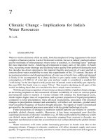
Figure 16.1 Plot of annual change in soil organic carbon (SOC)
over 10 years under conventional tillage and fully implemented
ridge tillage using initial SOC composition of calibrated stability
(02:41:57).
Soil Organic Carbon
0-20 cm
0.2
0.25
0.3
0.35
0.4
Time, yrs
CT
RT All
0246810
% 50C
© 2005 by Taylor & Francis Group, LLC
Soil Carbon Sequestration 415
those obtained by Coulibaly (i.e., Table 16.2). We also gener-
ated 10 years of daily weather data by interpolation between
nearest existing weather stations using MarkSim, version 1
(P. Jones et al., 2002). The generated daily data include rain-
fall, maximum temperature, minimum temperature, and
solar radiation. Small amounts of N (13 kg ha
−1
100 cm
−1
infiltrated rainfall) (Campbell, 1978; Pieri, 1992; Vitousek et
al., 1997) were applied to all simulated crops according to

infiltration of rainfall.
16.2.1.3 Agronomic Experiment Data
Agronomic yield trial data for a 3-year maize study were
obtained from Njti Coulibaly in Mali, including soil, weather,
and management of the crops in each year. That experiment
was simulated using the DSSAT CERES-Maize model, and
genetic coefficients were estimated using measured anthesis
dates and yields for the 3 years (Jones et al., 2002a). Data in
Table 16.2 demonstrate that the model describes anthesis
dates and yields across the 3 years with errors less than 10%.
Although additional tests are desirable, this exercise demon-
strated that the model can simulate growth and yield
responses to typical growing conditions in Mali under conven-
tional management.
Detailed measurements from experiments comparing RT
vs. CT were not available. Thus, a computer experiment was
conducted over a 10-year period: (1) to adjust field runoff
parameters for RT vs. CT, and (2) to compare predicted grain
and biomass yield values for RT and CT with those responses
Table 16.2 Calibration of Local Maize Variety Sotubaka:
Three Years of Observed and Simulated Grain Yield and
Days to Anthesis
Time to Anthesis (days) Maize Grain Yield (kg ha
−1
)
1999 2000 2001 1999 2000 2001
Simulated 62 61 57 5486 4138 5514
Observed 63 61 58 5100 3900 6070
Source: From Coulibaly, Ntji, personal communication, 2002.
© 2005 by Taylor & Francis Group, LLC

416 Jones et al.
reported by Gigou et al. (2000). Maize was planted each year
in the computer experiment as soon as the soil in the top 30
cm of soil reached 60% of plant available water, but no earlier
than June 18 to ensure adequate moisture for germination.
Harvest was assumed to occur at maturity, which was simu-
lated for each season. Plant density was set at three plants
m
−2
in all simulations, and row width was 75 cm. Crops sim-
ulated under CT had no manure or N fertilizer applications,
and 90% of the crop residue was removed after harvest. Man-
agement of RT included application of inorganic N (40 kg ha
–1
applied in two doses), return of 90% of crop residue to the
soil, and addition of 3 metric tons ha
−1
of (dry) manure.
Runoff parameters for the RT field were set by assuming
that the ridges were sufficiently constructed to reduce runoff
by 45% relative to CT management (M. Doumbia, personal
communication, 2003; Gigou et al., 2000). Runoff curve num-
bers of 90 and 96 were selected for RT and CT, respectively.
Simulated runoff for the 10 years was 45% less for RT vs. CT
management, and differences in yield and residue biomass
between CT and RT closely matched differences reported by
Gigou et al. (2000) (Table 16.3).
16.2.2 Simulation of Soil C Sequestration
Potential, RT vs. CT
After soil and crop parameters were adjusted to mimic CT vs.

RT as described above, simulated changes in SOC were com-
Table 16.3 Simulated Maize Grain and Biomass Production
Under CT and RT Plus Amendments and Percent Increase,
Compared with Similar Results in 2000 Study
Maize Grain (kg ha
−
1) Maize Biomass (kg ha
−
1)
CT RT % Increase CT RT % Increase
Simulated 10-year
average
2651 3565 34 6007 7750 29
Gigou et al. (2000) 2603 3599 38 6339 8704 37
Notes: CT = conventional tillage; RT = ridge tillage.
© 2005 by Taylor & Francis Group, LLC
pared over the 10 simulated years (Figure 16.1). SOC for CT
Soil Carbon Sequestration 417
remained nearly constant for the initial C fractions used in
the simulations but the RT-all treatment increased by 54%,
from 0.24% to 0.37% in the top 20 cm of soil over the 10 years
(10,527 to 7016 kg C ha
−

1
; bulk density was 1.44 g cm
3
). This
increase amounted to 3511 kg ha
−1

, or about 351 kg ha
−1
year
–1
, and was about 10% of the total carbon added to the
soil from residues and manure during the 10 years. This result
indicates that the potential for SOC sequestration for the
conditions studied may be less than the 0.20% increase that
was hypothesized, and less than the average rates for no till
vs. CT reported by West and Post (2002), but similar to values
obtained by Pichot et al. (1981) in Burkina Faso and by Lal
(2000) in the no-till treatment in Nigeria.
Two other treatments were simulated in the computer
experiment to estimate how much SOC sequestration would
occur under RT only (no amendments added), and under RT
with 40 kg ha
−1
N and return of 90% of crop residue (RT, Fl,
R, no manure addition). Data in Table 16.4 indicate that yield
increased under the RT only treatment, but that SOC did not
increase. Although roots added C to the soil in all treatments,
simulated results show that roots of maize alone would not
be enough to increase SOC in this environment. For RT plus
N fertilizer and residue return to the field, yield increased
about the same as for RT plus all amendments, but the SOC
increase was only 2058 kg ha
−1
, or about 60% of the amount
sequestered when manure was included.
Table 16.4 Grain Yield, Crop Residue, and Change in SOC

After 10 Years Under Each Management System
a
Treatment CT RT Only RT, F, R RT All
Mean grain yield (kg ha
−1
) 2651 3006 3592 3565
Mean harvest residue (kg ha
−1
) 6007 6875 7750 7751
Change in SOC (kg ha
−1
[10 year)
−1
]) −46 −355 2058 3511
Ending SOC (%) 0.24 0.23 0.32 0.37
a
For top 20 cm of soil, bulk density = 1.44 g cm
−3
.
Notes: CT = conventional tillage; F = 40 kg ha
–1
of N fertilizer added; R = 90%
of crop residue left on the field each year; RT = ridge tillage; SOC = soil organic
carbon.
© 2005 by Taylor & Francis Group, LLC
418 Jones et al.
These preliminary results agree with the trend observed
by Pieri (1992) in long-term studies in West Africa that, in
treatments without manure, soil C remained constant or
declined, and that fertilizer alone aggravated the condition.

This also agrees with the study in Western Nigeria (Lal,
1997a, 1997b), which illustrated the importance of residue
and tillage operations on SOC and maize grain yield. Under
those conditions, the no-till plus mulch treatment had the
greatest effect with a doubling of SOC during the first 4 years
of the study. However, it is notable that all treatments showed
initial increases followed by subsequent declines in SOC
within 8 years. Several important differences existed in his
study, however, namely, that average rainfall was higher
(1200 mm), two crops were planted each year and more fer-
tilizers were applied.
16.3 COMBINING MEASUREMENTS AND
MODELS FOR ESTIMATING SOC
SEQUESTRATION
If soil C sequestration is to become an accepted mechanism
for reducing atmospheric CO
2
levels, a soil carbon accounting
system needs to be developed (Antle and Uehara, 2002). Mass
of carbon accumulation in soils is of interest, so measurements
will include field sampling, laboratory determination of car-
bon, and its conversion to mass basis using soil bulk density.
Thus, errors in such measurements would include errors asso-
ciated with each step. As a result, yearly changes in soil C
are small relative to errors associated with the measurement
process, and such measurements are expensive. Biophysical
models can be used to estimate SOC and its changes under
different weather, soil, and management practices (Parton et
al., 1988, 1994; Jones et al., 2002b). However, although these
models may produce precise estimates, they are imperfect and

parameters for specific field situations are uncertain. Thus,
errors exist in estimates of SOC from field measurements and
from model predictions.
© 2005 by Taylor & Francis Group, LLC
Soil Carbon Sequestration 419
Techniques exist to combine models and measurements
to obtain better estimates of system states and model param-
eters. The Kalman filter (Maybeck, 1979; Welch and Bishop,
2002) approach first uses a model to predict the state of a
system, and then uses measurements to update the estimates
in an optimal way, taking into account errors in measure-
ments and predictions. Variations of the Kalman filter, origi-
nally developed for linear models, have been developed for
non linear models (e.g., Albiol et al., 1993; Graham, 2002).
One variation, the ensemble Kalman filter (Burgers et al.,
1998; Eknes and Evensen, 2002; Margulis et al., 2002), was
used by Jones et al. (2004) to evaluate its use for estimating
SOC and a decomposition rate parameter over time for a
single field using a nonlinear model.
Here the use of ensemble Kalman filter (EnKF) method-
ology to combine measurements with models to estimate SOC
is demonstrated. Analyses in this chapter focus on estimation
of SOC over time (years) for a single field following the work
of Jones et al. (2004); they do not address spatial variability
or aggregation of estimates over space.
16.3.1 Soil Carbon Model
A simple discrete-time model is used to simulate SOC (X
t
, kg
ha

−1
) as it changes over time, using a time step of 1 year. It
is assumed that only one pool of C exists in the soil, and that
biomass organic carbon (U
t
, kg ha
−1
) may increase this pool,
while during the same annual time step, microbial activity
decomposes both X
t
and U
t
. The model also has one parameter
(SOC decomposition rate constant, R, year
−1
) that is constant
over time, but is not known with certainty. The resulting
model has one state variable (X
t
) and one parameter (R),
which are estimated using the EnKF. Uncertainties in model
predictions of SOC and R are assumed. State equations for
the nonlinear, stochastic model follow:
X
t
= X
t–1
– R·X
t–1

+ b· U
t–1
+ ε
t
R = R
0
+ η (16.1)
© 2005 by Taylor & Francis Group, LLC
420 Jones et al.
where
X
t
= soil organic carbon in year t (kg[C] ha
−1
)
R=rate of decomposition of existing SOC (year
−1
)
R
0
= initial estimate of SOC decomposition rate (year
−1
)
b=fraction of fresh organic C that is added to the soil
in year t that remains after 1 year
U
t
=amount of C in crop biomass added to the soil in
year t (kg[C] ha
−1

year
−1
)
ε
t
=model error for SOC (kg[C] ha
−1
)
0 = error in estimate of decomposition rate R (year
−1
)
Model error (ε
t
) includes uncertainties in U and b, as well
as uncertainties due to the fact that the model is a simplifi-
cation of reality. It is also assumed that model and parameter
errors are normally distributed and uncorrelated. Thus,
ε
t
~ N(0, σ
ε
)
2
(16.2)
η ~ N(0, σ
η
)
2
where
σ

ε
2
= variance of model error for X
t
σ
η
2
= variance of model error for R
The model error (ε
t
) is a random process that changes over
time but is uncorrelated with time (i.e., white noise), whereas
decomposition rate parameter error (η) is a random variable
that does not change with time.
16.3.2 Soil Carbon Measurements
Soil C measurements (Z
t
) may be made each year or less
frequently, but measurements of R are not possible. Thus, the
model has two variables that are to be estimated, but only
one is observable. Furthermore, it is assumed that the SOC
measurement error is normally distributed, independent in
time and independent from X and R. A time series of mea-
surements was generated using two steps to demonstrate the
approach. First, a time series of true values of SOC (X
t
) was
computed using Equation 16.1 with the true value of the
parameter R for the hypothetical field. Then, a time series of
© 2005 by Taylor & Francis Group, LLC

Soil Carbon Sequestration 421
measurements was generated by randomly sampling from the
distribution of Z (ε
z
) and adding this random error to “true”
SOC values at each discrete time step. Thus, Z
t
was generated
by
Z
t
= X
t
+ ε
z,t
(16.3)
where
Z
t
= measurement of SOC in year t, kg[C]/ha
ε
z,t
= error in measurement, ε
z,t
~ N(0,σ
z
)
2
where σ
z

2
is variance of SOC measurement error. In real appli-
cations of the EnKF, actual measurements would be used.
16.3.3 The Ensemble Kalman Filter: Combining
Model and Measurements
The Kalman filter is a set of mathematical equations that are
used to obtain optimal estimates of the state of a system.
There are two types of equations in a Kalman filter: (1) time
update equations, and (2) measurement update equations
(Welch and Bishop, 2002). The time update equations project
forward in time the current predictions of the system state
and covariance. The measurement update equations provide
feedback by incorporating a new measurement to obtain an
improved estimate of system state and covariance. In a dis-
crete-time Kalman filter, a linear stochastic model is used to
project the state and covariance estimates forward to the next
time step. At measurement times, the model-projected state
and covariance values are updated by using the measurement
and its covariance characteristics. A Kalman gain matrix is
computed to update estimates of system state and covariance.
This process is repeated over time in a recursive fashion,
projecting values for each discrete time step and updating
those estimates for time steps when measurements are avail-
able.
The ensemble Kalman filter (EnKF) follows this same
general approach for nonlinear models, but relies on Monte
Carlo methods to project state and covariance values between
measurement times (Burgers et al., 1998; Marguilis et al.,
2002). The SOC model (Equation 16.1) is nonlinear due to
© 2005 by Taylor & Francis Group, LLC

422 Jones et al.
multiplication of R and X, and both “states” of the system are
estimated. The equations to update X
t
and R
t
at each time
step in the EnKF are:
Updated X
t
= Predicted X
t
+ K
X
(Z
t
− Predicted X
t
)
(16.4)
Updated R
t
= Predicted R
t
+ K
R
(Z
t
− Predicted X
t

)
where K
X
and K
R
are Kalman gains for X
t
and R
t
, computed
at each time that measurements are used to update the vari-
ables.
For this particular problem (i.e., the specific model, the
variables to be estimated, and the measurements that are
made), these gain factors can be computed as follows (Jones
et al., 2004):
(16.5)
where σ
X,t
2
is the variance of soil C predictions at time t, and
σ
XR,t
is the covariance between X and R estimates at time t.
These variance and covariance values are estimated before
state estimates are updated.
Note that although R is not measured, the measurement
of SOC provides information for refining the estimate of R via
the covariance term. Also note that these gains vary with
time; they are recalculated each time a measurement is made.

If measurements are not made in a particular year, model
predictions provide estimates of SOC and the update step is
omitted.
The Kalman gain variables are used to weight the
updated estimate on the basis of error variances. Note, for
example, that if measurement error variance (σ
Z
)
2
is very
small relative to model prediction variance (σ
X,t
),
2
then K
X
approaches 1.0, and the updated X
t
(Equation 16.4) will be
approximately the value (Z
t
) that was measured. In contrast,
if measurement error is large relative to prediction error, K
X
K
X
σ
Xt,
2
σ

Xt,
2
σ
Z
2
+
=
K
R
σ
XR,t
σ
Xt,
2
σ
Z
2
+
=
© 2005 by Taylor & Francis Group, LLC
Soil Carbon Sequestration 423
will be closer to 0.0, and the updated estimate will be near
the predicted value. Furthermore, if the covariance term used
to compute K
R
is small, the updated R
t
will remain near its
estimate from the previous step. However, if the covariance
term is large, differences between measured and predicted

SOC will result in adjustments to R in the update step.
16.3.4 Example Results
Jones et al. (2004) presented a sensitivity analysis to assess
the benefits of using this EnKF to estimate SOC over time,
relative to measurements alone, for different combinations of
model parameters, errors, and initial conditions. Here, base
case results from this study are summarized, and it is shown
how errors of SOC estimation vary over time under different
frequencies of measurements (and thus, frequencies of updat-
ing estimates of X and R).
To demonstrate numerical values, realistic parameters
and error terms were selected for a case study. The variance
of SOC measurements (σ
Z
)
2
was set at 500,000 (a standard
deviation of 707 kg[C] ha
−1
or a standard error of measure-
ment of 0.0253% C on a mass basis). The initial value of SOC
was assumed to be 16,000 kg[C] ha
−1
in the top 20 cm of soil,
which is about 0.6% carbon on a mass basis (Yost et al., 2002).
Variance of this initial SOC estimate was assumed to be
20,000 (kg[C] ha
−1
)
2

, a standard deviation of 141 kg[C] ha
−1
.
It was also assumed that the model error variance (σ
ε
)
2
was
20,000 (kg[C] ha
−1
)
2
. The value of R
0
was assumed to be 0.020
(based on a range of values reported by Pieri, 1992, and
Bationo et al., 2003); the variance in this parameter (σ
η
)
2
was
assumed to be 0.0001. The value of U
t
was set at a relatively
high value of 2000 kg[C] ha
−1
, constant across all years, and
the value of b at 0.20.
Equation 16.3 was used to generate measurements (Z
t

)
for t = 1 through 30 years for a hypothetical field for which
SOC is to be estimated, using an initial value of SOC of 16,000
kg[C]/ha and an R value of 0.010. The difference between
R
0
and R for a particular field conceptually represents the
variability among fields that belong to the population of fields
© 2005 by Taylor & Francis Group, LLC
424 Jones et al.
that has a mean value of R
0
. The updated estimates of R
t
should converge to the value for the specific field, starting
from the initial value of 0.020. The values of parameters and
initial conditions used to implement the EnKF are summa-
rized in Table 16.5. The EnKF was used to estimate X and R,
and their variances for each year of the 30 years for which
measurements were generated. Annual changes in SOC esti-
mated from measurements (Z
t
− Z
t−1
) and from EnKF esti-
mates (Updated X
t+1
− Updated X
t
), were compared with true

values that were generated.
used (Table 16.5), as well as annual measurements (generated
as discussed above), and “true” values of SOC for the 30-year
case study. Estimates made by the EnKF are smooth, and in
most years are closer to the “true” values than measured
values. Estimates of R evolved from an initial estimate of
0.020 year
−1
to values near the “true” value of 0.010 after
about 6 years (not shown), and remained near that value for
Table 16.5 Values of Parameters, Initial Conditions, and
Inputs for Example Ensemble Kalman Filter
Variable Definition Units Value
X
0
True value of soil organic carbon at time
0
kg[C]/ha 16,000
R True value of mineralization parameter 1/year 0.010
σ
Z
2
Variance of measurement, constant over
time
(kg[C]/ha)
2
500,000
σ
ε
2

Variance in model estimates of soil
organic carbon, each year time step
(kg[C]/ha)
2
20,000
R
0
Initial estimate of soil C decomposition
parameter
1/year 0.020
σ
η
2
Variance of decomposition rate
parameter
(1/year)
2
0.0001
U
t
Input of C to the soil each year (assumed
constant)
kg[C]/ha 2,000
b Proportion of annual soil C input that
remains after 1 year
— 0.20
Source: Adapted from Jones, J.W., W.D. Graham, D. Wallach, W.M. Bostick, and
J. Koo. 2004. Trans. ASAE, 47(1):331–339.
© 2005 by Taylor & Francis Group, LLC
Figure 16.2 shows EnKF estimates of SOC for the inputs

Soil Carbon Sequestration 425
the remainder of time in the case study. The effect of the
EnKF is clear when one compares annual changes in SOC
annual changes were closer to “true” values in all years except
one (year 10). EnKF estimates of annual changes in SOC were
improved more than estimates of SOC vs. time when com-
pared with measurements because of the smoothing process
that occurs when model estimates are combined with mea-
surements.
Three additional runs were made to demonstrate the
effect of measurement frequency on standard error of SOC
estimates. Errors for measurements made every year, every
2 years, every 3 years, and every 5 years are shown in
obtained from using measurements alone (707 kg ha
−1
). These
results indicate that SOC estimation errors using the EnKF
and measurements every 3 years would be less than errors
based on measurements alone. They also show that errors in
SOC estimates decrease over time, after an initial increase,
Figure 16.2 Changes in soil organic carbon (SOC) over time based
on measurements (open symbols) and EnKF (heavy line) compared
with “true” values of SOC (light line). (Modified from Jones, J.W.,
W.D. Graham, D. Wallach, W.M. Bostick, and J. Koo. 2004. Trans.
ASAE, 47(1):331–339.)
12000
14000
16000
18000
20000

22000
24000
051015 20 25 30 35
Years
Soil C (kg ha
-1
)
© 2005 by Taylor & Francis Group, LLC
(Figure 16.3). Over the 30-year study, the EnKF estimates of
Figure 16.4. Also shown is the standard error of SOC estimate
426 Jones et al.
Figure 16.3 Annual changes in soil organic carbon comparing
EnKF estimates with measured and true values. (Modified from
Jones, J.W., W.D. Graham, D. Wallach, W.M. Bostick, and J. Koo.
2004. Trans. ASAE, 47(1):331–339.)
Figure 16.4 Effect of measurement frequency on errors of soil
organic carbon (SOC) estimates. The heavy dashed line is the stan-
dard error of SOC estimates based on measurements alone. (Modi-
fied from Jones, J.W., W.D. Graham, D. Wallach, W.M. Bostick, and
J. Koo. 2004. Trans. ASAE, 47(1):331–339.)
1
3
5
7
9
11
13
15
17
19

21
23
25
27
29
Year
Annual changes in SOC, kg ha
-1
Measured EnKF Estimates True Values
-1500
-1000
-500
0
500
1000
1500
2000
0
200
400
600
800
1000
1200
051015 20 25 30 35
Years
Standard error of soil C
estimates (kg ha
-1
)

Meas = 1:1 Year
Meas = 1:2 Years
Meas = 1:3 Years
Meas = 1:5 Years
© 2005 by Taylor & Francis Group, LLC
Soil Carbon Sequestration 427
which is the result of more accurate estimates of R and lower
model prediction error. Jones et al. (2004) reported on a more
comprehensive analysis of the EnKF under different combi-
nations of parameters, initial conditions, and errors in model
and measurements. They found that estimates of SOC were
better than measurements alone in all combinations when
this simple model was used in the EnKF, although estimation
errors decreased more under some combinations than others.
16.4 DISCUSSION
In this chapter, two types of model uses related to SOC seques-
tration were demonstrated. In the first one, a model was used
to perform computer experiments to evaluate SOC sequestra-
tion potential as affected by different management practices
in a particular location in Mali. Although data were limited
for this region, the example demonstrated the value of using
available data to adapt a model before using it to evaluate
alternative management practices in a region. When the com-
puter experiment was conducted using the same DSSAT
maize model, but without using local data to adapt the model,
results were clearly inconsistent with known yield and runoff
responses of RT vs. CT and to realistic changes in SOC. Obvi-
ously more data and more work are needed to improve pre-
dictions and confidence in simulated results. Nevertheless,
the preliminary estimates of SOC sequestration obtained in

this study are certainly reasonable. They fall within the range
of values reported elsewhere (see West and Post, 2002; Pichot
et al., 1981; Lal, 2000), and simulations of runoff and yield
of maize in RT vs. CT are consistent with local data and
knowledge.
The second example represents a new use of biophysical
models. The motivation for this use was that reliable esti-
mates of SOC sequestration will be needed if landowners
enter into contracts in which they are paid to sequester an
agreed upon amount of carbon. In this case, a model was used
to integrate measurements over time to improve estimates of
SOC sequestration using an ensemble Kalman filter. This
procedure also improved model predictions over time (errors
© 2005 by Taylor & Francis Group, LLC
428 Jones et al.
were reduced) as new measurements were used, and a model
parameter was more accurately estimated for the particular
field. Through the recursive combination of model predictions
and new observations, the model was better adapted to predict
SOC levels at the specific site.
The second example showed the need for knowing errors
associated with model predictions, and it demonstrated how
to include uncertainties (stochastic features) in models for
this purpose. The demonstration of this data assimilation
technique was limited to a single field and to the use of a
simple model. However, this approach is amenable to the use
of more complex models, including the DSSAT-CENTURY
model used in the first example. Koo et al. (2003) and Bostick
et al. (2003) showed that one can use the EnKF to assimilate
both crop biomass and SOC measurements to improve esti-

mates of SOC using more complex models. This approach
lends itself to the use of remote sensing data to improve SOC
estimates by assimilating biomass data over space and time.
Although the case study presented was for a single field, the
EnKF can be expanded to estimate SOC over large areas that
would be required in a carbon contract. This capability is
currently being developed, following similar developments in
the field of hydrology (Graham, 2002). This approach appears
to have potential for other practical applications as well.
Crop and soil models can be very useful tools in SOC
sequestration studies. But, they can also be misused. The
phrase “all models are wrong; some are useful” is important
to keep in mind. The main theme of this paper was the impor-
tance of using local data, however scarce, with such models
to help better understand and predict SOC sequestration
responses to soil, climate, and management. The procedure
used to integrate local data with models was referred to as
model adaptation. One aspect of that adaptation process is
the estimation of soil, crop, and management parameters that
allow the model to predict important variables for application
to the problem being addressed. This process is sometimes
referred to as model calibration, which may invoke criticisms
from those whose aim is to have models that do not require
© 2005 by Taylor & Francis Group, LLC
Soil Carbon Sequestration 429
modifications in order to predict system performance. Cer-
tainly, more work is needed to improve model capabilities;
this will always be true. However, the diversity and spatial
variability of land management, soils, climate, and genetic
composition of crops will always create challenges to those

who need to tailor agricultural management systems to
achieve goals of individual farmers and of society. In this
chapter, it has been shown that existing models can be used
effectively to better understand and predict SOC sequestra-
tion. The importance of both data and models needs to be
recognized as efforts are made to improve knowledge and tools
for use in science and policymaking.
ACKNOWLEDGMENTS
This research is supported by the Soil Management Collabo-
rative Research Program (SM CRSP) through a grant (LAG-
G-00-97-00002-00) from the U.S. Agency for International
Development and by a grant from the National Aeronautics
and Space Administration titled “Carbon from Communities:
A Satellite View” (Florida Agricultural Experiment Station
Journal Series N-02376).
REFERENCES
Albiol, J., J. Robuste, C. Casas, and M. Poch. 1993. Biomass estima-
tion in plant cell cultures using an extended Kalman filter.
Biotechnol. Prog., 9:174–178.
Anderson, J.M. and J.S.I. Ingram. 1993. Tropical Soil Biology and
Fertility: A Handbook of Methods. CAB International, Walling-
ford, UK.
Antle, J.M. and G. Uehara. 2002. Creating incentives for sustainable
agriculture: defining, estimating potential, and verifying com-
pliance with carbon contracts for soil carbon projects in devel-
oping countries. In A Soil Carbon Accounting System for
Emissions Trading. Special Publication SM CRSP 2002–4. Uni-
versity of Hawaii, Honolulu, HI, pp. 1–12.
© 2005 by Taylor & Francis Group, LLC
430 Jones et al.

Bationo, A., U. Mokwunye, P.L.G. Vlek, S. Koala, and B.I. Shapiro.
2003. Soil fertility management for sustainable land use in the
West African Sudano-Sahelian zone. In Gichuru, M.P., A.
Bationo, M.A. Bekunda, H.C. Goma, P.L. Mafongonya, D.N.
Mugendi, et al., Eds. Soil Fertility Management in Africa: A
Regional Perspective. Academy Science Publishers, Nairobi, pp.
253–292.
Bielders, C.L., P. Baveye, L.P. Wilding, L.R. Drees, and C. Valentin.
1996. Tillage-induced spatial distribution of surface crusts on
a sandy paleustult from Togo. Soil Sci. Soc. Am. J., 60:843–855.
Bostick, W.M., J. Koo, J.W. Jones, A.J. Gijsman, P.S. Traore, and B.V.
Bado. 2003. Combining Model Estimates and Measurements
Through an Ensemble Kalman Filter to Estimate Carbon
Sequestration. ASAE Paper 033042. American Society of Agri-
cultural Engineers, St. Joseph, MI.
Burgers, G., P.J. van Leeuwen, and G. Evensen. 1998. Analysis
scheme in the Ensemble Kalman Filter. Monthly Weather Rev.,
126:1719–1724.
Campbell, K.L. 1978. Pollution in Runoff from Nonpoint Sources.
Water Resources Research Center. University of Florida,
Gainesville.
Cole, C.V., J. Williams, M. Shaffer, and J. Hanson. 1987. Nutrient
and organic matter dynamics as components of agricultural
production systems models. In Soil Fertility and Organic Matter
as Critical Components of Production Systems. Special Publica-
tion 19, Soil Science Society of America/American Society of
Agronomy, Madison, WI, pp. 147–166.
Coulibaly, Ntji. 2002. Personal communication, September 5, IER,
Sotuba, Bamako, Mali.
Daba, S. 1999. Note on effects of soil surface crust on the grain yield

of sorghum (Sorghum bicolor) in the Sahel. Field Crops Res.,
61:193–199.
Doumbia, M. 2003. Personal communication. SM CRSP Annual
Review, February 17, Bambey, Senegal.
du Toit, A.S., J. Booysen, and J.J. Human. 1998. Calibration of
CERES3 (maize) to improve silking date prediction values. S.
Afr. J. Plant Soil, 15:61–65.
© 2005 by Taylor & Francis Group, LLC