GIS Based Studies in the Humanities and Social Sciences - Chpater 10 doc

139

10

A Toolbox for Spatial Analysis on a Network

Atsuyuki Okabe, Kei-ichi Okunuki, and Shino Shiode
CONTENTS

10.1 Introduction 139
10.2 Tools in SANET 141
10.3 Software and Data Setting 142
10.4 Network

K

Function Method 144
10.5 Network Variable-Clumping Method 146
10.6 Network Cross

K

Function Method 148
10.7 Network Voronoi Diagram 148
10.8 Network Huff Model 149
10.9 Conclusion 151
Acknowledgments 151
References 151

10.1 Introduction

In the real world, we notice many events and situations that locate at specific
points on a network. These are referred to as

network spatial events

. Some typical
examples relevant to studies in the humanities and social sciences are as follows:
Homeless people living on the streets (Arapoglou, 2004).
Street crime (Harries, 1999; Painter, 1994; Ratcliffe, 2002).
Graffiti sites along streets (Bandaranaike, 2003).
Urban cholera transmission (Snow, 1855).
Traffic accidents (Yamada and Thill, 2004).
Illegal parking (Cope, 1990).
Street food stalls (Stavric, 1995; Tinker, 1997).

2713_C010.fm Page 139 Friday, September 2, 2005 7:32 AM
Copyright © 2006 Taylor & Francis Group, LLC

140

GIS-based Studies in the Humanities and Social Sciences

In addition to the types of events listed above, there is another large class
also representing network spatial events, but these occur alongside a net-
work. A typical example is shown in Figure 10.1, where the circles indicate
the locations of churches in Shibuya-Shinjuku, Tokyo. It can be seen that
these are not freely situated over the region, since their positions are strongly

constrained by their location along the streets.
Not only churches, but also almost all facilities in an urbanized area, are
located at the side of streets, and it is actually the gates or entrances of these
facilities that lie adjacent to the thoroughfare.
This chapter focuses on the analysis of events and facilities that are placed
at specific locations on and alongside a network, and are called

network
spatial events

.
A decade ago, analysis of network spatial events was very difficult,
because network data were poor and there were few tools for their analysis,
such that researchers had to assemble data and develop methods them-
selves. This task demanded much time and effort. The modern advent of
geographical information systems (GIS) and the abundance of network
data that are accessible today have, fortunately, made matters easier, and
many GIS-based tools are available. In this chapter, we introduce a user-
friendly toolbox, called SANET, which is the abbreviated name for Spatial
Analysis on a Network. This tool is useful for answering, for instance, the
following questions:
Does illegal parking tend to occur uniformly in no-parking streets?
Are street crime locations clustered in “hot spots”?
Do fast-food shops tend to contend with each other?

FIGURE 10.1

Churches alongside the streets in Shibuya-Shinjuku, Tokyo.

2713_C010.fm Page 140 Friday, September 2, 2005 7:32 AM

Copyright © 2006 Taylor & Francis Group, LLC

A Toolbox for Spatial Analysis on a Network

141
How extensive is the service area of a post office?
What is the probability of consumers choosing a particular down-
town store?
In the subsequent sections, we show how to answer these questions using
SANET.

10.2 Tools in SANET

SANET was released in November 2001, and it has been evolving ever since
(Okabe, Okunuki, and Shiode, 2004). The current 2005 edition of SANET is
the third version, and it provides the following 15 tools:
1. Construction of a node-adjacency data set.
2. Assignment of a data point to the nearest point on a network.
3. Aggregation of attribute values belonging to the same item.
4. Generation of a network Voronoi diagram.
5. Generation of random points on a network.
6. Enactment of the network cross

K

function method.
7. Enactment of the network

K

function method.
8. Partition of a polyline into constituent line segments.
9. Assignment of polygon attributes to the nearest line segment.
10. Enactment of the nearest-neighbor distance method.
11. Enactment of the conditional nearest-neighbor distance method.
12. Calculation of polygon centroids.
13. Enactment of the network Huff model.
14. Enactment of the variable clumping method.
15. Comparison of two networks.
In the subsequent sections, the procedure for spatial analysis on a net-
work using these tools is outlined. First, in Section 10.3,

SANET

and datasets
set up on the computer are described. Second, in Sections 10.4–10.8, we
show how to achieve spatial analysis with the network

K

function method
(Tool 7) using an illustrative example in Figure 10.1; also shown are the
network variable-clumping method (Tool 14), the network cross

K

function
method (Tool 6), the network Voronoi diagram (Tool 4), and the network
Huff model (Tool 13).

2713_C010.fm Page 141 Friday, September 2, 2005 7:32 AM
Copyright © 2006 Taylor & Francis Group, LLC

142

GIS-based Studies in the Humanities and Social Sciences

10.3 Software and Data Setting

The software SANET consists of two components: the main program, and
the interface between this and a GIS viewer.
The main program performs the geometric and algebraic computation
needed for running the tools mentioned in Section 2. This program works
independently, and can, in theory, be interfaced with any GIS viewer. The
interface between the main program and a viewer will clearly depend on
the choice made from the many viewers available. SANET currently adopts
ArcView, which is one of the most popular GIS viewers. The main program
and the interface can be downloaded from the SANET Web site: http://
okabe.t.u-tokyo.ac.jp/okabelab/atsu/sanet/sanet-index.html.
This download can be made without charge for nonprofit-making uses. Also
posted on this Web site is the detailed manual of SANET and information
about the most recent version. The GIS viewer ArcView is obtainable at a
reasonable price from Environmental Systems Research Institute, Inc. (ESRI).
After installing both SANET and ArcView on a personal computer, the
computer-readable digital data of a street network and churches has to be
obtained. There are many ways of recording and managing the digital data
of a street network. The main program of SANET employs adjacent-node tables

that are commonly used in computational geometry. The adjacent-node
tables for the street network of Figure 10.2 are shown in Table 10.1. This

illustration consists of straight-line segments whose end points (called

nodes

)
are labeled by numbers. Table 10.1(a), called a

header table

, shows that node

i

, say node 0, is headed to the ID

=

0 in Table 10.1(b). Table 10.1(b) shows
that the nodes adjacent to the node corresponding to ID

=

0 (i.e., node 0) are
nodes 1 and 5 (reading downwards).

FIGURE 10.2

Nodes of a street network.
9
5

4
2
1
0
10
491

2713_C010.fm Page 142 Friday, September 2, 2005 7:32 AM
Copyright © 2006 Taylor & Francis Group, LLC

A Toolbox for Spatial Analysis on a Network

143
The structure of street data varies in differing GIS software packages.
ArcView uses Polyline, which is not compatible with the adjacent-node
tables. Therefore, when SANET is used, we have to transform Polyline to
enable it to function. This transformation is made by using Tool 1.
The digital data for churches may be given either as the coordinates of
their representative centroid points or as polygons representing the areas
occupied by the buildings. SANET assumes that features are represented by
points. With data given in the latter form, the centroids of the polygons are
easily located by using Tool 12.
For SANET, all network spatial events are precisely on a network. As is
seen in Figure 10.1, churches are not exactly located on streets, because a
point does not indicate the gate of a church but the centroid of its buildings.
In practice, these entrance data are difficult to obtain, and, hence, we have
to estimate them from the centroids. SANET assumes that the nearest point
on a street from the centroid of a facility is its gate. The location of these
access points

is derived by using Tool 2. An example is given in Figure 10.3,
which shows the access points of the churches plotted in Figure 10.1.



TABLE 10.1

Adjacent Node Tables

(a) Header table

(b) Adjacent node table
Node ID Head ID Adjacent Node



000 1
121 5
252 0
383 2
4 11 4 491

FIGURE 10.3

The access points of churches in Shibuya-Shinjuku, Tokyo, obtained using Tool 2.

2713_C010.fm Page 143 Friday, September 2, 2005 7:32 AM
Copyright © 2006 Taylor & Francis Group, LLC

144

GIS-based Studies in the Humanities and Social Sciences

We are ready to analyze network spatial events, now that SANET and the
data are set up.

10.4 Network

K

Function Method

When observing the distribution of churches in Shibuya-Shinjuku, seen in
Figure 10.3, we wonder whether they are clustered, random, or dispersed.
There are many methods available for this analysis, and SANET provides
two tools to enable the determination to be performed. These methods are
the

K

-function (Tool 7), and the nearest-neighbor distance (Tool 10). The first
of these approaches is used below.
The

K

-function method was originally formulated on a plane by Ripley
(1981), and this was extended by Okabe and Yamada (2001) to apply to a
network. The K

-function is formulated in terms of the function defined
as the cumulative number of points representing events within the shortest-
path distance

t

, from a point, ,

i

=

1,…

n

, where

n is the number of points.
For example, the bold lines in Figure 10.4 indicate the sub-network in which
the distance from is less than or equal to 1000 meters. Since two churches,
represented by the two circles on the bold lines, are located on this sub-
network, the value of for

t

=

1000 meters is two, i.e.,

K

1

(1000)

=

2. By
extending

t

from 0 to 7000, we obtain the function as in Figure 10.5.
In terms of , the

K -function, , is written as:
(10.1)

FIGURE 10.4

The sub-network in which the distance from is less than or equal to 1000 meters.
p
1
p
1
Kt
i
()
p

i
p
1
Kt
1
()
Kt
1
()
Kt
i
() Kt()
Kt
n
Kt
i
i
n
() ()=
=
∑
1
1

2713_C010.fm Page 144 Friday, September 2, 2005 7:32 AM
Copyright © 2006 Taylor & Francis Group, LLC

A Toolbox for Spatial Analysis on a Network

145

This implies that the

K

function is the average of the functions across

i

=

1…

n

.
To examine whether the churches tend to be clustered or dispersed, the

observed



K

-function, which is obtained from given data, is compared with
the

expected K

-function obtained when spatial-event points are uniformly
and randomly distributed over the network. Figure 10.6 shows such a real-

ized set of points for the streets in Shibuya-Shinjuku using Tool 5 (the number
of points is the same as that in Figure 10.3). To obtain the expected

K

function,
as many as 1000 sets of points are generated, and the resulting

K

functions
are averaged to give the approximate expected result.
Figure 10.7 shows the observed

K

function and the expected

K

function
for the churches in Shibuya-Shinjuku, obtained by using Tool 7. The observed

K

function (the black curve) is always above the expected

K

function (the

FIGURE 10.5

function for the church at in Figure 10.4.

FIGURE 10.6

Randomly and uniformly generated points on the streets in Shibuya-Shinjuku, Tokyo, using
Tool 5 (the number of points is the same as that in Figure 10.1).
10
20
2
30
40
50
60
70
80
90
0 1000 2000 3000 4000 5000 6000 7000 8000
Kt
1
() p
1
Kt
i
()

2713_C010.fm Page 145 Friday, September 2, 2005 7:32 AM
Copyright © 2006 Taylor & Francis Group, LLC

146

GIS-based Studies in the Humanities and Social Sciences

gray curve). This implies that the churches in Shibuya-Shinjuku tend to be
clustered rather than randomly distributed.

10.5 Network Variable-Clumping Method

The finding in Section 10.4 suggests that there may be a distinct pattern of
“clumps” in the distribution of churches in Shibuya-Shinjuku. To examine
whether or not such a pattern exists, the variable-clumping method (Tool
14) is employed. The clumping method on a plane, originally devised by
Roach (1968), was developed into the variable-clumping method on a plane
by Okabe and Funamoto (2000), and extended to a network by Shiode and
Okabe (2004).
To explain the meaning of a “clump,” we define the

r-neighborhood

of a
point, , as the sub-network of a network in which the shortest-path dis-
tance from to any point in the

r

-neighborhood is less than or equal to

r

,
which is called the

clump radius

. The

r

-neighborhood of is indicated by
the bold, gray line in Figure 10.8. A

clump

is a set of points whose

r

-neigh-
borhoods form one connected sub-network of a network (Figure 10.8). The
number of points forming a clump are referred to as the

clump size

. This
varies from 1, (one point forms one “clump”); to

n

(all the points form one
clump). The state of clumping, called the

clump state

and denoted by ,
is described in terms of the number, , of clumps with respect to clump
size,

k

, that is:
(10.2)

FIGURE 10.7

The observed (the black curve) and expected (the gray curve)

K

functions for churches in
Shibuya-Shinjuku, Tokyo.
0
10
20
30
40
50
60
70

80
90
0 2000 4000 6000 8000 10000 12000 14000
p
i
p
i
p
1
Cr()
Nk r(|)
Cr N r N r Nn r() ( (|), (|), , (|))= 12…

2713_C010.fm Page 146 Friday, September 2, 2005 7:32 AM
Copyright © 2006 Taylor & Francis Group, LLC

A Toolbox for Spatial Analysis on a Network

147
Since in Figure
10.8, the clump state of the points in Figure 10.8 is = (2, 3, 1, 0, 0, 0, 0,
0, 0, 0, 0).
In the above, the clump radius

r

is constant, but it can be variable. The
method of describing the clump state from the smallest to the largest value
of

r

is called the

variable-clumping method

. In this way, local clumps, and also
global clumps, can be shown.
Among many possible clump states, there is a need to detect “significant”
ones. A

significant clump state

is defined as that one which rarely occurs (i.e.,
occurs with small probability) in the context of points being uniformly and
randomly distributed over a network. The significant clump states can be
discerned by generating random points many times using Tool 5. Figure 10.9
shows one of the significant clump states observed in the distribution of
churches in Shibuya-Shinjuku, which was detected by using Tool 14. The
clump radius is 500 meters, and the probability of realizing a pattern like

FIGURE 10.8

Clumps with radius

r

.

FIGURE 10.9

A significant clump state observed in the distribution of churches in Shibuya-Shinjuku, Tokyo.
r

p
1

size 2
size 1
size 2
size 2
size 1

size 3

2r

Nr N r N r Nir i(|),(|),(|),(|), ,,122331 041=====K 11
Cr()

2713_C010.fm Page 147 Friday, September 2, 2005 7:32 AM
Copyright © 2006 Taylor & Francis Group, LLC

148

GIS-based Studies in the Humanities and Social Sciences

Figure 10.9 is less than 0.05. This significant clump state is characterized by
one clump of size 18, one clump of size 5, five clumps of size 3, 10 clumps
of size 2, and 24 clumps of size 1; in particular, the clump of size 18 is

distinctive.

10.6 Network Cross

K

Function Method

The observation in Section 10.4 may suggest that the churches tend to be
located around transport stations. This trend can be examined by the net-
work cross

K

function method (Tool 6) formulated by Okabe and Yamada
(2002), which is an extension of the cross

K

function method defined on a
plane.
The cross

K function method is similar to the K function method mentioned
in Section 10.3.2, but the root points are different. The sets of points consid-
ered are those of churches, , and of stations, . A func-
tion, , is defined as the cumulative number of churches within the
shortest-path distance, t, from a station, , i = 1… m, where m is the number
of stations. The cross K function is defined by:
(10.3)

If churches tend to cluster around stations, the observed cross K function
for the given two sets of points will be larger than the expected cross K
function to be obtained if churches are uniformly and randomly distributed.
In the case of the K function method, the expected function is obtained
from random Monte Carlo simulations, but in the case of the cross K function
method, the expected function is analytically obtained. This was shown by
Okabe and Yamada (2002).
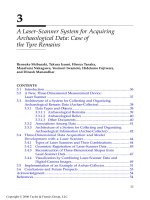
Figure 10.10 shows the observed cross K function (the black line) and the
expected cross K function (the gray line) for the churches and stations in
Shibuya-Shinjuku. The black line is above the gray line within 5000 meters,
and it is therefore concluded that churches in this area tend to be clustered
around transport stations.
10.7 Network Voronoi Diagram
In spatial analysis, there is often a need to estimate the service areas of
facilities, such as post offices. Precise estimation is not easy, but a first approx-
imation can be derived from the network Voronoi diagram (Okabe et al.,
pp
n1
,,…
qq
m1
,,…
Kt
i
C
()
q
i
Kt
m

Kt
C
i
C
i
m
() ()=
=
∑
1
1
2713_C010.fm Page 148 Friday, September 2, 2005 7:32 AM
Copyright © 2006 Taylor & Francis Group, LLC
A Toolbox for Spatial Analysis on a Network 149
2000). In definition of this, let be post offices located on the street
network N, and be the shortest-path distance from an arbitrary
point on the network N to a post office at . In these terms, we define a
sub-network, , as:
, i = 1,… m, (10.4)
implying a sub-network in which the nearest post office is . The network
Voronoi diagram, V, for the generator points is the set of the result-
ing sub-networks, i.e., . If it is assumed that residents
use the post office nearest to their homes, shows the service area of
the post office at .
Figure 10.11 shows an example of the network Voronoi diagram con-
structed using Tool 4. The black circles are the post offices in Shibuya, and
the white circles indicate the boundary points between two adjacent Voronoi
sub-networks.
10.8 Network Huff Model
One of the most important tasks in retail marketing is to estimate the prob-

ability of consumers electing to buy at a particular store selected from among
many such stores in a city. The Huff model (1963) provides this choice
probability. The model was originally formulated on a plane and later
extended to a network by Miller (1994) and Okabe and Okunuki (2001).
To set out the network Huff model explicitly, consumers’ houses are con-
sidered located at , and stores lie at on a street network.
FIGURE 10.10
The observed cross K function (the black line) and the expected cross K function (the gray line)
of churches with respect to stations in Shibuya-Shinjuku, Tokyo.
0
500
1000
1500
2000
2500
3000
0 500 1000 1500 2000 2500 3000 3500 4000 4500 5000
qq
m1
,,…
dpq
i
(, )
p q
i
Vq
i
(
)
Vq p dpq dp q i jj m

iij
() {|(,) (|), , , , }=≤≠=1 …
q
i
qq
m1
,,…
VVq Vq
m
= { ( ), , ( )}
1
…
Vq
i
()
q
i
pp
n1
,,… qq
m1
,,…
2713_C010.fm Page 149 Friday, September 2, 2005 7:32 AM
Copyright © 2006 Taylor & Francis Group, LLC
150 GIS-based Studies in the Humanities and Social Sciences
Let be the shortest-path distance from a house at to a store at ,
and is the magnitude of attractiveness (e.g., the floor area) of the store
at . The probability, , of a consumer at choosing the store at
among the m stores is given by:
(10.5)

Tool 13 computes this probability. Figure 10.12 shows an example where
the squares indicate stores, and the density of gray tint indicates the proba-
FIGURE 10.11
Network Voronoi diagram of post offices (black circles) in Shibuya, Tokyo. White circles indicate
the boundary points between two adjacent Voronoi sub-networks.
FIGURE 10.12
Probability of the store at the large square being chosen. Small squares mark the other stores.
dp q
ij
(,) p
i
q
j
a
j
q
j
Pp q
ij
(,)
p
i
q
j
Pp q
adpq
adpq
ij
jij
kik

k
m
(,)
/( , )
/( , )
=
=
∑
α
α
1
2713_C010.fm Page 150 Friday, September 2, 2005 7:32 AM
Copyright © 2006 Taylor & Francis Group, LLC
A Toolbox for Spatial Analysis on a Network 151
bility of the store at the large square being chosen. Black indicates a high
probability.
10.9 Conclusion
Although, as shown in the introduction, there are numerous network spatial
events that attract study by scholars of the humanities and social sciences,
spatial analysis of those events began only recently (e.g., Yamada and Thill,
2004; Spooner et al., 2004). One reason for this delay was a lack of tools.
SANET now provides a toolbox to assist researchers who wish to analyze
spatial events on a network. We hope to hear about successful applications
of SANET.
Acknowledgments
We thank T. Ishitomi, K. Okano, and C. Mizuta at Mathematical Program-
ming Co., Ltd. for coding SANET. This development was partly supported
by Grant-in-aid for Scientific Research No. 10202201 of the Ministry of Edu-
cation, Culture, Sports, Science and Technology of Japan.
References

Arapoglou, V., The governance of homelessness in the European South: spatial and
institutional contexts of philanthropy in Athens, Urb. Stud., 41, 621–639(19),
2004.
Bandaranaike, S., Graffiti hotspots: physical environment or human dimension, Graf-
fiti and Disorder Conference convened by the Australian Institute of Criminol-
ogy in conjunction with the Australian Local Government Association,
Brisbane, 2003.
Cope, J.G. and Allred, L.J., Illegal parking in handicapped zones: demographic ob-
servations and review of the literature, Rehabil. Psychol., 35, 249–257, 1990.
Harries, K., Mapping Crime: Principle and Practice, National Institute of Justice (NIJ)
Crime Mapping Research Report, U.S. Department of Justice, NCJ 178919, 1999.
Huff, D. L., A probabilistic analysis of shopping center trade area, Land Econ., 39,
81–90, 1963.
Miller, H.J., Market area delimitation within networks using geographic information
systems, Geogr. Sys., 1, 157–173, 1994.
Okabe, A., Boots, B., Sugihara, K., and Chin, S-N., Spatial Tessellations: Concepts and
Applications of Voronoi Diagrams, 2nd ed., John Wiley, Chichester, 2000.
2713_C010.fm Page 151 Friday, September 2, 2005 7:32 AM
Copyright © 2006 Taylor & Francis Group, LLC
152 GIS-based Studies in the Humanities and Social Sciences
Okabe, A. and Funamoto, S., An exploratory method for detecting multi-level clumps
in the distribution of points — a computational tool, VCM (variable clumping
method), J. Geogr. Sys., 2, 111–120, 2000.
Okabe, A. and Okunuki, K., A Computational Method for Estimating the Demand
of Retail Stores on a Street Network Using GIS, Trans. GIS, 5(3), 209–220, 2001.
Okabe, A., Okunuki, K., and Shiode, S., SANET: A toolbox for spatial analysis on a
network, Geogr. Anal., 2005 (to appear).
Okabe, A. and Yamada, I., The K function method on a network and its computational
implementation, Geogr. Anal., 33, 271–290, 2001.
Painter, K., The impact of street lighting on crime, fear, and pedestrian street use,

Secur. J., 5, 116–24, 1994.
Ratcliffe, H.J., Aoristic signatures and the spatio-temporal analysis of high volume
crime patterns, J. Quant. Crim., 18, 23–43, 2002.
Ripley, B.D., Spatial Statistics, John Wiley & Sons, New York, 1981.
Roach, S.A., The Theory of Random Clumping, London, Methuen, 1968.
Shiode, S. and Okabe, A., Network variable clumping method for analyzing point
patterns on a network, AAG annual meeting, Philadelphia, 2004.
Snow, J., On the Mode of Communication of Cholera, 2nd ed., Churchhill Livingstone,
London, 1855.
Spooner, P.G., Lunt, I.D., Okabe, A., and Shiode, S., Spatial analysis of roadside Acacia
populations on a road network using the network K function. Land. Ecol., 19(5),
491–499, 2004.
Stavric, B., Matula, T.I., Klassen, R., and Downie, R.H., Evaluation of hamburgers
and hot dogs for the presence of mutagens, Food Chem. Toxicol., 33, 15–820, 1995.
Tinker, I., Street Foods: Urban Food and Employment in Developing Countries, Oxford
University Press, New York, 1997.
Yamada, I. and Thill, J-C., Comparison of planar and network K functions in traffic
accident analysis, J. Trans. Geogr., 12(2), 149–158, 2004.
2713_C010.fm Page 152 Friday, September 2, 2005 7:32 AM
Copyright © 2006 Taylor & Francis Group, LLC