HANDBOOK OF SCALING METHODS IN AQUATIC ECOLOGY MEASUREMENT, ANALYSIS, SIMULATION - PART 2 ppt

65
5
Acoustic Remote Sensing of Photosynthetic Activity
in Seagrass Beds
Jean-Pierre Hermand
CONTENTS
5.1 Introduction 66
5.2 Inßuence of Photosynthesis on Acoustics 67
5.2.1 Bubbles in Seawater 67
5.2.2
Posidonia Photosynthetic Apparatus 69
5.2.3 Oxygen Production 69
5.2.4 Gas in Matte and Sediment 69
5.3 The
USTICA 99 Experiment 69
5.3.1 Test Site 69
5.3.2 Experimental ConÞguration 71
5.3.3 Acoustic Measurements 72
5.3.3.1 Signal Transmission 72
5.3.3.2 Ambient Noise Recording 72
5.3.3.3 Transducer Calibration 72
5.3.3.4 Equalized Matched-Filter Processing 73
5.3.4 Oceanographic Measurements: CTD and Dissolved Oxygen Content 73
5.4 Multiscale Acoustic Effects 75
5.4.1 Time-Varying Medium Impulse Response 75
5.4.2 Propagation Channel Modeling 77
5.4.3 Energy Time Distribution of Medium Response 80
5.4.4 Non-Photosynthesis-Related Effects 81
5.4.4.1 Tide 81
5.4.4.2 Sea Surface Motion 82
5.4.4.3 Water Temperature ProÞle 83

5.5 Effects of Photosynthesis on Sound Propagation 83
5.5.1 Time Variation of Dissolved Oxygen 83
5.5.2 Effect of Photosynthetic Bubbles on Multipaths 84
5.5.3 Effect on Reverberation 88
5.5.4 Effect on Ambient Noise 88
5.5.4.1 Spectral Characteristics 88
5.5.4.2 Time-Frequency Characteristics 90
5.5.4.3 Directional Characteristics 91
5.5.4.4 Other Observations 91
5.5.5 Gaseous Interchange of the Leaf Blade 91
5.6 Conclusion 92
Acknowledgments 93
Appendix 5.A Comparison with Earlier Experiments 94
References 94
© 2004 by CRC Press LLC
66 Handbook of Scaling Methods in Aquatic Ecology: Measurement, Analysis, Simulation
5.1 Introduction
To be able to prevent damage to marine and freshwater ecosystems, for example, to avert negative
consequences for biodiversity, environmental surveillance and monitoring tools are required that produce
data that are continuous in time and representative of extended areas of interest. In recent years, research
on acoustic remote sensing of the ocean has evolved considerably, especially in studying physical and
biological processes in shallow water environments.
1
Methods and systems have been developed that
exploit, to different degrees, the complex nature of sound propagation to identify physical and biological
markers (parameters) of the water column, its boundaries, and subbottom structures. Among these,
sophisticated acoustic inversion techniques based on matched Þeld and matched waveform processing
have proved effective and reliable in determining range-average physical properties of the water column
and upper sediments.
2–4

This chapter focuses on the use of acoustics to remotely sense biological processes through an original
case study: the photosynthesis by
Posidonia oceanica (L.) Delile, an endemic marine phanerogam of
the Mediterranean Sea. The organism settles most commonly on loose sediments but can develop on
hard and rocky substrata and, when it encounters favorable conditions, colonizes vast areas of the sea
bottom forming prairies, which extend from the surface to a depth of approximately 35 to 40 m. The
prairies represent the most characteristic and, probably, most important ecosystem of the Mediterranean
Sea covering an estimated surface area of 20,000 square miles. They are an important habitat for numerous
Þsh species, marine animals, and other species of plants and algae. They create natural barriers that reduce
coastal erosion.
Posidonia is called the “green lung of the Mediterranean” for its important characteristic
of producing large quantities of oxygen. Unfortunately, the plants are sensitive to environmental decay
and have suffered marked regression over the last 40 years. The development of methods to assess their
state of health efÞciently is of considerable interest as traditional direct methods, e.g., underwater diving
for inspection and sampling, and indirect methods, e.g., mechanical and high-frequency echographic
An exploratory study was started in 1995 to Þnd ways of monitoring
in situ, and on the scale of a
prairie,
the response of Posidonia plants to environmental conditions.
10
To this end, the effects of
photosynthesis on long-range propagation of low frequency sound were investigated under controlled
experimental conditions.
11,12
Transmission measurements in the frequency range 100 Hz to 1.6 kHz
showed daily changes of frequency-dependent propagation characteristics including attenuation and
dispersion (pulse spreading). The diurnal variations were attributed in part to undissolved gas present
on the leaf blades during phases of photosynthesis cycle. A previously unsuspected phenomenon of
waveguide propagation of sound in a bottom bubble layer was discovered, and it was shown that the

phenomenon could be exploited to determine the oxygen void fraction in that layer. The proposed acoustic
sampling is not invasive; i.e., it does not affect the metabolism of the plant and, in particular, the gaseous
exchange with the ambient medium in ways that, for example, an incubator enclosing the plant does.
The method preserves the natural life condition allowing us to obtain qualitative information about the
plant response to environmental variables such as photosynthetically active radiation (light), temperature,
stirring, and nutrients. Furthermore, the method alleviates the problem of space and time aliasing
associated with traditional spot measurements. The acoustic propagation data “integrate” the acoustic
effect of a great number of plants present along the source–receiver transect of arbitrary length within
the prairie of interest. A static conÞguration of the transducers allows observation over long time periods
(days to months) and at short time intervals (minutes to seconds), covering a great number of photo-
synthesis cycles.
In this chapter, we report and discuss results from a second experiment carried out under completely
different conditions with respect to the Þrst experiment in terms of the measurement geometry, acoustic
transmission, and environment. The major differences were the much shorter length of acoustic path,
broader frequency range of transmission, much lower oxygen productivity of the plants, lower plant
density, lesser homogeneity of the prairie, and acoustically harder rocky substratum. The experiment
was conducted in September 1999 over a small
Posidonia bed off the island of Ustica. Time series of
calibrated measurements of acoustic transmission were obtained during 4 days using broadband chirp
© 2004 by CRC Press LLC
soundings, require considerable time and/or costly equipment; see, e.g., References 5 through 9.
Acoustic Remote Sensing of Photosynthetic Activity in Seagrass Beds 67
signals emitted repeatedly from an underwater sound source and received on a pair of hydrophones,
Þxed near the sea bottom. Contemporaneous depth proÞles and time series of dissolved oxygen and
temperature in the water column were obtained with an oceanographic probe. Statistical analyses of the
time-varying, medium impulse response allow to resolve marked changes in the propagation characteris-
tics. Photosynthesis is seen to cause excess attenuation of multipaths, faster decay of reverberation, and
lower level of ambient noise. There is a strong correlation with the release of oxygen in the water column
measured with the dissolved oxygen probe. As for the Þrst experiment, the diurnal variations are ascribed
in part to undissolved gases present on the leaf blades and at the roots during phases of photosynthesis

cycle. The
Posidonia plants form a water layer where the gas void fraction varies with the time of day.
The photosynthesis-driven, absorptive, scattering, and dispersive bubble layer, with a sound speed lower
than bubble-free water, modiÞes the interaction process of waterborne acoustic energy with the substra-
tum of volcanic basalt. Multipaths with intermediate grazing angles are shown to be the most sensitive
to photosynthesis.
Section 5.2 brießy reviews the morphological features of
Posidonia that are relevant to bubble
acoustics. Section 5.3 describes the
USTICA 99 experiment and data processing. In Section 5.4, the
acoustical and environmental measurements are analyzed in detail. Section 5.5 focuses on the effects of
photosynthesis on acoustic propagation including multipaths, reverberation, and ambient noise and
provides an interpretation of the observed acoustic variations in terms of the gas transport in the seagrass.
of the two experiments are compared.
In the conÞnes of a single chapter we Þnd it necessary to omit or pass quickly over certain notions
of ocean acoustics and signal theory. Interested readers are referred to the referenced textbooks.
5.2 Inßuence of Photosynthesis on Acoustics
In coastal waters, the gas content in dissolved and bubble forms is determined by air–sea ßux and speciÞc
environmental and biomass conditions including photosynthesis of aquatic plants, life processes of
animals, and decomposition of organic materials.
5.2.1 Bubbles in Seawater
It is well established that the presence of gas bubbles in seawater inßuences sound propagation in a way
that depends on the resonant frequency of the bubbles.
13,14
In coastal waters, the presence of bubbles of many sizes, each with (sound) scattering and absorption
cross sections,
*
cause frequency-dependent scatter, attenuation, and dispersion. Bubble radii are in the
range 10 to 500
mm with a peak density typically somewhere in the range 10 to 15 mm. Recently

published observations, using laser holography near the ocean surface, have shown that the densities of
10 to 15
mm radius bubbles can be as high as 10
6
m
–3
mm
–1
increment within 3 m of the surface of calm
seas.
15
The density and distribution of bubble radius vary with depth, time of day, season, wind, and sea
biological processes in the volume and on the seaßoor, which are quite speciÞc to each environment
such as photosynthesis considered in this chapter.
Typically, bubbles form only a very small percentage, by volume, of the sea in which they occur.
Nevertheless, because air, or more generally gas, has a markedly different density and compressibility
than seawater, and because of the resonant characteristics of bubbles, the suspended gas content has a
profound effect on underwater sound. At frequencies of resonance, gas bubbles pulsate radially in
response to a signal frequency dependent on bubble radius. For a spherical air bubble in water a
simpliÞed
**
expression of the resonant (breathing) frequency is as follows:
*
Ratio of the scattered power, referred to a unit distance, to the intensity incident on a unit area (or unit volume).
**
i.e., no surface tension, adiabatic gas oscillation and no energy absorption.
© 2004 by CRC Press LLC
state (see, e.g., References 16 and 17). The bubble population is sensitive to the physical, chemical, and
Section 5.6 concludes the chapter. In Appendix 5.A, the acoustic parameters and environmental conditions
68 Handbook of Scaling Methods in Aquatic Ecology: Measurement, Analysis, Simulation

(5.1)
where
a is the bubble radius in mm, z is the depth in m, and k is the wavenumber.
*
For example, a bubble
of radius 100
mm near the sea surface resonates at a frequency of ª32.5 kHz. The extinction (scattering
plus absorption) cross section has a maximum at the resonant frequency and falls off with frequency
away from the resonance. Well below the resonance the cross section increases as
f
4
. Bubbles of near-
resonant size extract a large amount of energy from the incident sound wave through scattering in all
directions and conversion to heat. Also, in the vicinity of resonance, large changes in sound speed take
place. Hence, over the range of resonance frequencies the medium is highly attenuative and dispersive.
18
By contrast, at high frequencies well beyond the resonant frequency of the smallest bubble present in
the mixture, the effect of suspended gas content is negligible. At frequencies below resonance, the
mixture of bubbles increases the compressibility of the water medium thereby reducing the sound speed
below that obtained from pressure, temperature, and salinity measurements alone.
**
When gas is dissolved
FIGURE 5.1 Posidonia oceanica leaves. (A) Adult and intermediate leaves covered by epiphytes and encrustation.
(B) Juvenile leaves and rhizome. (Underwater photographs taken during
USTICA
99 experiments).
FIGURE 5.2 Photosynthesis apparatus of P. oceanica. Leaf blade cross sections. (A, B) Monolayered epidermidis and
mesophyll with large cells and small intercellular spaces (¥320 and ¥200). PC: phenolic cell. (C) Detail of the porous
region under the cuticle (¥1100). (From P. Colombo, N. Rascio, and F. Cinelli, Posidonia oceanica (L.) Delile: a structural
study of the photosynthetic apparatus, Mar. Ecol., 4(2), 133–145, 1983. With permission.)

*
k = 2p/l [radians/m] where l [m] is the wavelength. The wavenumber and angular frequency w = 2pf [radians/s] are related
through the equation k = w/c where c [m/s] is the speed of sound.
**
Sound speed is related to density and compressibility and, in the ocean, density is related to static pressure, salinity, and
temperature. Sound speed is an increasing function of temperature, salinity, and pressure, with the latter a function of depth.
It is customary to express sound speed c as an empirical function of three independent variables: temperature T in °C,
salinity S in parts per thousand, and depth z in m. A simpliÞed expression for this dependence is c = 1449.2 + 4.6T – 0.055T
2
+ 0.00029T
3
+ (1.34 – 0.01T)(S – 35) + 0.016z.
19
A BC
f
a
zka
r
ª
¥
+
()
<<
325 10
101 1
6
12
.
. for
© 2004 by CRC Press LLC

Acoustic Remote Sensing of Photosynthetic Activity in Seagrass Beds 69
in water the effect on sound speed is completely negligible, even when the water is completely saturated
with gas.
20
5.2.2 Posidonia Photosynthetic Apparatus
Posidonia oceanica (L.) Delile is an endemic phanerogam of the Mediterranean Sea. Its long ribbon-
shaped leaves are grouped in shoots, which develop on various substrates in 1 to 50 m water depths
medium. The leaf blade consists of a monolayered epidermis and a three- to four-layered mesophyll
21
The major site of photosynthesis is the epidermis where chloroplasts are densely arranged in small
radially elongated cells. The outer wall of epidermidal cells is formed by an outer continuous layer
(cuticle) and an underlying much thicker (
ª20 mm) porous region with irregularly shaped cavities. The
lacunar system is constituted of connected air channels within the mesophyll. The particularly small
dimensions of the lacunar system is a distinctive feature of
P. oceanica.
Photosynthesis is the major driving force for exchange of gases among seawater, the epidermal cells,
the lacunar system. Unlike other aquatic plants, gaseous exchanges with seawater are effected by
molecular diffusion as there are no stomata. The processes of oxygen uptake for respiration and release
of photosynthetic oxygen are constrained by the diffusion boundary (unstirred) layer, and to a lesser
extent, by the cuticle and cell wall.
5.2.3 Oxygen Production
Photosynthesis by seagrass substantially increases the quantity of oxygen in dissolved and bubble forms
in the water column. For
Posidonia, a productivity of 5 to 10 g of Þxed carbon m
–2
day
–1
was reported.
22

Values of up to 14 l m
–2
day
–1
of produced oxygen have been reported for prairies of the Tuscan
Arcipelago.
23
Specialized surveys showed that the time variation of oxygen concentration in the water
column was determined principally by the daily cycle of oxygen productivity, with depth and seasonal
dependence, including the possible occurrence of supersaturation conditions below sea surface.
11,24
5.2.4 Gas in Matte and Sediment
The Posidonia matte is formed by the intertwining of various strata of rhyzomes, roots, and trapped
sediments.
25
Typically, the sediments are made of poorly sorted sands, primarily organogenous.
The geoacoustic properties of the matte are virtually unknown. Attenuation is known to be high as
acoustic energy of a boomer hardly penetrates the matte layer owing to scattering and absorption. Sound
speed is expected to be low due to the uneven nature of water-saturated loose sediments and to the
presence of slow materials (rhyzomes and roots) and gas from the decomposition of organic material.
For signal frequencies below the bubble resonances the bulk material properties of the matte is expected
to dominate its mechanical behavior, producing an acoustic response equivalent to a monophasic material
of low sound speed. Comparable conditions are encountered with soft porous sediments with high gas
5.3 The
USTICA
99 Experiment
5.3.1 Test Site
The experiment was conducted over a Posidonia bed off the island of Ustica in September 1999
of 65 km from Palermo (13°10
¢ E, 38°42¢ N). It represents the relict of a vast submarine volcanic system

of the Pleistocene age, which emerged 2000 m above the seabottom.
27,28
The island is characterized by
© 2004 by CRC Press LLC
(Figure 5.1). Leaf morphology allows for maximum release of photosynthetic oxygen to the ambient
and the lacunar system. Respiratory activity is nearly an order of magnitude lower and largely involves
(Figure 5.2). The blade width and thickness are respectively ª1 cm and ª180 mm.
(Figure 5.3A). The island lies in the southern Tyrrhenian Sea, off the northern coast of Sicily, at a distance
content (see, e.g., Reference 26).
70 Handbook of Scaling Methods in Aquatic Ecology: Measurement, Analysis, Simulation
pillow-shaped outcrops of lava emerging from the sea surface. It has an area of 8 km
2
, a coastal perimeter
of 12 km, and a summit elevation of 248 m. The coast is irregular and fretted, forming little inlets like
the one where the experiment was conducted (Figure 5.3B).
The island is surrounded by notably clear waters, which are subject to intense renewal, and seabeds
abundant with marine ßora and fauna in an ecosystem still practically intact and now protected.
*
The
seabed is settled by benthic communities typical of hard substrata. Marine vegetation includes surface
FIGURE 5.3 Test site. (A) Geological marine map of Ustica island showing the location of the investigated Posidonia
bed. (B) Sediments, biocenosis, and stratigraphy at the test site. The thick black line shows the position of the acoustic
transect. S: source. R: receivers. (Adapted from Reference 48.)
*
Since 1986, a marine reserve has been established, covering an area of 3 miles from the coast.
© 2004 by CRC Press LLC
Acoustic Remote Sensing of Photosynthetic Activity in Seagrass Beds 71
formations, hard calcareous algae, and various species of the seaweed Cystoseira distributed over the
water depths 0 to 35 m. The most euphotic sandy and subhorizontal bottoms are carpeted by the seagrass
P. oceanica (0 to 30 m). The deep rocky seabed, which is washed by intense currents, is capped with

dense oceanic settlements of
Laminaria rodriguezi (50 to 70 m). The marine fauna is very rich and can
be deemed as representative of the Central Mediterranean basin, with a notable host of subtropical forms.
The richness of the encrusting biocoenoses is the most noticeable feature of the island’s seascape.
5.3.2 Experimental Configuration
A sound source (S) and a pair of receivers (R1, R2) were deployed on the seaßoor (Figure 5.4). The
positions were chosen to minimize bathymetric variations between S and R and the acoustical effects
of nearby rock scatterers and coastal reßectors. The S–R horizontal distance was
R = 53 m and the
water depth,
d, in the vertical section varied in the range 8 to 8.8 m.
The source was a broadband piezoelectric transducer mounted in a ballasted tower and positioned at
a height
H
S
= 1.55 m above the seaßoor (Figure 5.5). The monopole-like source has a frequency range
FIGURE 5.4 Experimental conÞguration for the acoustic remote sensing of undissolved oxygen produced by Posidonia
photosynthesis. The positions of the underwater sound source (S) and hydrophones (R1, R2) are indicated. Eigenray diagram:
The lines are the acoustic rays joining S and R1. Ray groups 1 through 10 are displayed. The black lines are the early
arrivals of groups 1 and 2. The thin black line is one of the four paths belonging to group 10: nine reßections at each of
the boundaries. S: surface; B: bottom; R: reßected; M: multiple. Horizontal scale 1:400. Vertical scale 1:200.
FIGURE 5.5 Acoustic instrumentation deployed on the seagrass bed. (A) Sound-source tower, rear view. (B) Two-hydrophone
vertical pole, front view.
AB
© 2004 by CRC Press LLC
72 Handbook of Scaling Methods in Aquatic Ecology: Measurement, Analysis, Simulation
of 200 Hz to 20 kHz and is omnidirectional up to 2 kHz. It was cable-connected through an impedance
transformer to a power driving ampliÞer and signal generator in the laboratory, located on shore, several
hundred meters uphill.
The receivers were two calibrated hydrophones mounted on a rigid pole and decoupled mechanically.

A hydrophone (R1) was positioned within the
Posidonia leaf layer and the other (R2) in the water layer,
at respective heights of
H
R1
= 0.3 m and H
R2
= 1.7 m above the seaßoor. The hydrophone signals were
ampliÞed and bandpass-Þltered with a high-pass RC Þlter and third-order Bessel Þlter f
–3dB
= 500 Hz
and a low-pass eight-order linear phase Þlter f
–3dB
= 16.7 kHz. The signals, carried by analog symmetric
lines, were recorded by a portable data acquisition unit.
The acoustic instrumentation was deployed by two divers with the support of a local Þshing boat and
a work boat.
5.3.3 Acoustic Measurements
5.3.3.1 Signal Transmission — The coded signal, s(t), transmitted to measure the band-limited
impulse response of the acoustic channel, g(t), consisted of a low-power, long duration, linearly frequency
modulated (LFM) waveform:
(5.2)
where
f
0
= 8.1 kHz, Df = 15.8 kHz, and Dt = 15.8 s (5.3)
Re stands for real part, rect is the rectangular function, f
0
is the carrier frequency, Df is the bandwidth,
and Dt is the duration. The frequency range is from f

1
= 200 Hz to f
2
= 16 kHz. Pulse compression was
achieved through the use of a correlation receiver or matched Þlter (MF) whose impulse response is the
same as the waveform of the signal emitted by the source, reversed in time. The large time-bandwidth
product, DtDf ª 2.5·10
5
, permitted to resolve closely spaced multipath arrivals with a sufÞcient ratio of
peak to ambient noise in spite of the limited power of the sound source, 180 dB mPa
–1
re 1 m at resonance
(940 Hz). The pulse repetition rate was Þxed at 1 ppm to obtain sufÞcient statistics in sampling the
physical and biological processes over the timescales of interest. About 3 · 10
3
probe signals were trans-
mitted over a 4-day period.
The reader is referred to the original paper
29
for a conceptual description of the coded signal and its
matched Þlter, to, e.g., References 30 through 32 for related theory of signal detection and estimation
and optimum Þltering, and to, e.g., References 33 and 34 for aspects of digital signal processing that
are relevant to this chapter. Further details are found in References 4, 35, and 36 that deal speciÞcally
with the application of broadband, LFM-coded signals and MF receivers to inverse problems including
the geoacoustic characterization of Þne-grained sediments in shallow water.
5.3.3.2 Ambient Noise Recording — Physical and biological sounds were recorded during the
“silent” intervals of the acoustic transmissions.
5.3.3.3 Transducer Calibration — The transducers and electronics of the S and R chains were
calibrated in situ after the experiments. A pole-mounted hydrophone was repositioned on the source axis
at a distance R

0
= 1.93 m and the probe signal was retransmitted.
requirement for precise measurements of the forward acoustic propagation. The Þrst bottom and surface
bounces are recognized at time delays t = 1 ms and t = 7 ms.
The surface-reßected signal displayed variability due to surface motion. The ª20-dB attenuation is
somewhat larger than the spherical spreading loss calculated from the calibration geometry, i.e.,
20log(R/R
0
) = 16.4 dB where R = 13.05 m, due to the frequency-dependent source directivity and
surface scattering loss. The bottom-reßected signal was strongly attenuated (>>5.4 dB geometrical
loss) since the grazing angle q = 58° was beyond the expected critical angle of the basalt interface
st t t j ft t j ft
()
=
()
()
()
[]
Re exp exprect DDDpp
2
0
2
© 2004 by CRC Press LLC
Figure 5.6 shows that the transmitted waveform was perfectly reproducible, which was an important
Acoustic Remote Sensing of Photosynthetic Activity in Seagrass Beds 73
and there was a two-way, excess attenuation due to photosynthesis in the intervening seagrass layer
as discussed subsequently.
5.3.3.4 Equalized Matched-Filter Processing —
was used to design the reference signal of an MF receiver that compensated for amplitude and phase
distortion of the source.

1. Hanning windowing was applied to the MF waveform to reduce the local bottom and surface
echoes.
2. The transmitting sensitivity response, measured on the radiation axis (Figure 5.7B) was equalized
for ßat spectrum. An inverse, Þnite impulse response (IFIR) Þlter was designed on the basis of
a frequency-decimated version of the source spectrum magnitude.
3. The source waveform was convolved with the IFIR Þlter, which, in the frequency domain, is
equivalent to multiplying by the IFIR squared magnitude with zero-phase distortion.
4. The resulting reference signal, time reversed, was convolved with the received signals.
In Figure 5.7C, raw and equalized MF (EMF) outputs are compared for one realization of the received
signal. The Þrst multipath arrivals, which were not identiÞed in the MF output, were perfectly resolved
in the EMF output, recovering the time resolution limit, 1/Df = 63 ms. The EMF output represents the
convolution of the transmitted autocorrelation function (sinc function) with the actual impulse response
of the medium. For the encountered conditions of limited source peak-power and high-level background
noise, the achieved processing gain allowed estimation of (the coherent part of) the medium response
as if the source transmitted an ideal high-energy pulse.
5.3.4 Oceanographic Measurements: CTD and Dissolved Oxygen Content
multiparameter, oceanographic probe Idromar IM51-201. Depth proÞles and time series were alternated
to obtain vertical and temporal sampling of the water column. For most time series, the probe sensors
concentration at the sea surface and seaßoor. The conductivity (salinity) was nearly homogeneous over
the whole water column with mild time variability, S = 37.8 – 38 ppt. The probe was deployed at a short
FIGURE 5.6
the stability of the transmission. The hydrophone was placed at an axial distance R
0
= 1.93 m which largely satisÞed the
far Þeld condition: R
0
> pa
2
/l
2

= 0.46 m, where a = 0.12 m is the radius of the circular piston source, c = 1538.5 m/s

is
the sound speed near the bottom and l
2
= c/f
2
= 9.6 cm is the shortest transmitted wavelength. The dotted lines indicate
the delays of the Þrst bottom and surface echoes, calculated from the geometry.
0 1 5 7 10 15
–1
0
1
Time (ms)
Amplitude
43 Time series overlaid
© 2004 by CRC Press LLC
Matched, Þltered pressure signal measured in front of the source. The overlaid, 43 signal realizations show
The emitted pressure waveform (Figure 5.7A)
were positioned just above the Posidonia leaves. Figure 5.8 shows the depth proÞles of temperature and
Physical and chemical conditions of seawater were monitored during the acoustic transmissions with a
oxygen concentration at different times of day. Figure 5.9 shows time series of temperature and oxygen
74 Handbook of Scaling Methods in Aquatic Ecology: Measurement, Analysis, Simulation
FIGURE 5.7 Equalized MF processing. (A) Raw MF transmitted signal (gray line) and Hanning (dashed) windowed
version (black). (B) Spectrum magnitude in dB (thick, right scale); ideal (thin, left scale), and designed (dashed) inverse
Þlter response. (C) Comparison of raw (gray line) and equalized (black) MF signal received on hydrophone R1. D, SR,
and BR stand for direct, surface- and bottom-reßected paths, respectively.
FIGURE 5.8 Depth proÞles of (A) temperature and (B) oxygen concentration at different times of day. Gray circles: raw
data; solid lines: smoothed data; dotted lines: references at T = 25.5°C and C
O

= 6 mg/l for visual appraisal of the depth
and time variations. The arrows indicate the direction of oxygen variation near the bottom (time-series part of the proÞles).
0 5 10 15
–1
0
1
Time (ms)
Amplitude
10
2
10
3
10
4
–70
–60
–50
–40
–30
–20
–10
0
Frequency (Hz)
Magnitude (dB)
0
1
Magnitude
–1 0 1 2 3 4 5
–1
0

1
Time (ms)
Amplitude
D
BR
SR
AB
C
08:04
08:37
09:04
09:37
09:58
10:24
15:44
16:15
17:37
18:11
19:16
19:49
20:12
20:51
21:07
21:37
06:18
06:49
10:06
10:34
12:20
12:38

12:39
13:09
15:08
15:32
17:48
18:33
19:41
20:18
0
5
10
06:58
07:34
D (m)
25 25.5 26
20:34
20:41
T (
5.5 6 6.5
O
2
(mg/l)
0
5
10
D (m)
Sept. 23, 1999 Sept. 24, 1999
A
B
© 2004 by CRC Press LLC

Acoustic Remote Sensing of Photosynthetic Activity in Seagrass Beds 75
distance off the transect to avoid acoustic reßections from the hull of the Þshing boat, which explains
the deeper depths in the displayed data.
5.4 Multiscale Acoustic Effects
In this section, the time history of acoustic transmission data is analyzed to assess their sensitivity to
the time variations of all environmental parameters that are relevant to acoustic frequencies below 16 kHz.
5.4.1 Time-Varying Medium Impulse Response
Changes in the physical and biological properties of the very shallow water environment are conveniently
related to the characteristics of the transmitted acoustic signals through the establishment of the time-
varying impulse response of the medium.
*
by 1-min intervals. The Þrst 4 ms of the envelope
**
of the EMF output are displayed. The envelope
representation is chosen here to highlight the temporal structure of the received energy.
***
The real-
FIGURE 5.9 Time series of (A) temperature and (B) oxygen concentration. The small circles are the raw data. Gray circles:
near the sea surface; dark circles: near the bottom. The surface and bottom data are in the depth ranges z £ 1 m and z ≥ 8 m,
*
Herewith and henceforth referred to as geotime.
**
Magnitude of the analytical signal calculated by Hilbert transform.
***
More precisely, the coherent component of the coded-signal energy transmitted through the medium.
18 00 06 12 18 00 06 12 18 00 06 12
25.2
25.4
25.6
25.8

26
26.2
T (° C)
18 00 06 12 18 00 06 12 18 00 06 12
5.5
6
6.5
Geotime (h)
O
2
(mg/l)
–3
–2
–1
0
+1
+2
Energy (dB)
A
B
Surface
Bottom
Bottom
Acoustic
O
2
Probe
© 2004 by CRC Press LLC
respectively. The dashed line in (B) replicates the acoustic result of Figure 5.18(A) for comparison (right scale).
Figure 5.10 shows the leading part of the medium response as a function of time of day separated

valued response was shown, for one realization, in Figure 5.7C. The leading part of the response shows
76 Handbook of Scaling Methods in Aquatic Ecology: Measurement, Analysis, Simulation
distinct arrivals, which were fairly stable from one signal to the next. The remaining part of the response,
which will be shown later, displayed much greater signal-to-signal variability and sensitivity to the time-
varying environmental conditions.
The static properties of the acoustic propagation channel were determined by (1) the range and depths
of the source and receivers, (2) the bathymetry, and (3) the acoustic properties of the basement. The
dynamic properties were the function of (4) the tidal cycle, (5) the sea state and wind speed, and of the
depth-dependent (6) temperature, (7) Þsh populations, and (8) gas bubbles in the water column. These
processes operated on different timescales and caused both deterministic and stochastic ßuctuations of
the medium acoustic-impulse response.
FIGURE 5.10 Geotime stack of 1-min-spaced acoustic-impulse response of the medium measured on hydrophone R1.
The responses were aligned in time using the real-valued peak of the Þrst arrival (D path) as reference. The envelopes are
displayed. The white regions are missing data. Period: September 22, 1913 hours to September 25, 1301 hours, 1999.
–0.5 0 0.5 1 1.5 2 2.5 3 3.5




18





00

06





12





18





00





06

12





18





00





06





12


Time (ms)
Geotime (h)

25 Sept 1999
24 Sept 1999
23 Sept 1999
© 2004 by CRC Press LLC
Acoustic Remote Sensing of Photosynthetic Activity in Seagrass Beds 77
5.4.2 Propagation Channel Modeling
For acoustic modeling purposes, the environment is described as an horizontally layered medium formed
by the water layer, leaf layer (Posidonia plants), rhyzomes/roots and trapped sediment layer (matte),
underlying sediment layers, and a semi-inÞnite half space (rock basement).
11
There are different theoretical (and computational) ways of describing the propagation of sound in
the ocean. Normal-mode theory
37
is particularly suited for shallow water but gives little insight, compared
to ray theory, on the distribution in space and time of the energy radiating from the source. Like its
analog in optics, ray acoustics provides a more intuitive description of the propagation in the form of a
*
for isospeed water and ßat boundary conditions. Under these simplifying assumptions the rays follow
straight lines in the water column and, at the boundaries, are specularly (mirror) reßected with the same
angle relative to the vertical.
In the experimental area, the Posidonia plants grow directly on a rocky substratum. They form a real
prairie, relatively dense and in good state of health. The average thickness of the leaf layer is 60 cm. In
is scarce and, when present, in small cavities, is thin and made of loose sediments with a predominance
of bioclast. The organogenous debris come from erosion of the substratum and bioactivities. The matte-
sediment composite layer is thin (a few centimeters) compared to most of the transmitted wavelengths
and thus was considered acoustically transparent. The substratum is a volcanic basalt that supports both
compressional and shear waves with speeds smaller than the typical values c
p
= 5250 m/s and
c

s
= 2500 m/s,
38
due to the young age of formation and subsequent alteration of the material.
Let us Þrst assume that the seabed vegetation is acoustically transparent. For an ideal hard bottom,
i.e., a non-absorbing material with a sound speed larger than water, there is “total reßection” of the
acoustic rays with grazing angles smaller than a critical value. For basalt, the apparent critical angle is
approximately
(5.4)
where c
w
= 1538.5 m/s is the sound speed of the bottom water, assumed bubble free, and c
b
= c
s
= 2000 m/s
since in consolidated materials for which c
s
> c
w
the shear speed takes on the role of compressional
speed in unconsolidated sediments.
37
The shear wave provides an additional degree of freedom for the
acoustic energy to penetrate into the bottom so that the interface appears “softer” than the equivalent
liquid layer (compressional wave only).
C
angle, in terms of the reßection loss and phase shift:
dB and (5.5)
calculated with a seismo-acoustic propagation model.

39
For a homogeneous bottom the reßection loss
near the horizontal within an aperture of 2q
c
suffers only a moderate loss increasing with angle due to
the lossy properties of the basalt. For an ideal, nonlossy material, there would be a perfect reßection
of the rays with subcritical incidence, i.e., no bottom loss. Outside this aperture a substantial part of
the energy is transmitted into the bottom at each bounce, which results in a strong decay with range
larger than at the steeper angles because of the elastic properties of the basalt. The small-scale roughness
of the actual bottom, not accounted for in the predicted mirrorlike reßection loss of Figure 5.11A,
causes an additional loss due to scattering, increasing with frequency and extending to lower and higher
grazing angles.
Figure 5.12 shows the 4-day average of the medium impulse response measured between S and R1. The
logarithm of the envelope is displayed because of the large dynamic range. The leading part of the response
*
Ray-based models lack accuracy in predicting the low-frequency part of the propagation because of the inherent (high fre-
quency) approximation.
q
cwb
cc=
()
ª ∞
-
cos
1
40
RR
dB C
=-20log ( )q f=
[]

-
tan Im( ) / Re( )
1
RR
CC
© 2004 by CRC Press LLC
ray diagram. In Figure 5.4 the acoustic rays joining the source S and receiver R1 (eigenrays) are traced
The curves in Figure 5.11A show the complex-valued, elastic reßection coefÞcient R vs. grazing
of the reßected component (Figure 5.12). The bottom loss at the intermediate angles 40° < q < 70° is
contrast to the previous experiment (see Appendix 5.A), there is not a real matte spreading. The matte
and phase shift curves are independent of frequency. Referring to Figure 5.4, energy that propagates
78 Handbook of Scaling Methods in Aquatic Ecology: Measurement, Analysis, Simulation
FIGURE 5.11 (A) Reßection coefÞcient vs. grazing angle and frequency. solid and dotted lines: Frequency-independent
loss in dB and phase shift of a half-space basalt bottom (left scales). Plot: Frequency-dependent loss of a composite seagrass-
basalt bottom during active photosynthesis (right and top scales). The basalt geoacoustic parameters used for the calculation
are compressional speed c
p
= 5000 m/s, shear speed c
s
= 2000 m/s, compressional attenuation a
p
= 0.2 dB/l, shear attenuation
a
s
= 0.5 dB/l and relative density r
b
/r
w
= 2.2. The water sound speed is c
w

= 1538.5 m/s. The sound speed of the bubble
seagrass layer is c
B
= 1264 m/s corresponding to a gas void fraction U = 5 ◊ 10
–5
. The bottom roughness and attenuation
in the seagrass layer are not accounted for. (B) ModiÞed grazing angle at the basalt bottom for different values of the gas
void fraction U in the seagrass layer. Corresponding sound speeds c
B
are indicated.
123456
2
3
4
(dB)
Grazin
g angle (degrees)
0102030405060708090
0
1
2
3
4
5
6
Loss (dB)
Log(
f
)
–180

–90
0
90
180
Phase angle (degrees)
0 10 20 30 40 50 60 70 80 90
0
10
20
30
40
50
60
70
80
90
θ
w
(degrees)
θ
B
(degrees)
U
= 5 × 10
–4
10
–4
10
–5
0

5 × 10
–5
c
B
= 638 m/s
1098
1264
1469
1538
A
B
© 2004 by CRC Press LLC
Acoustic Remote Sensing of Photosynthetic Activity in Seagrass Beds 79
and scattering at the surface and bottom boundaries, which produce a long reverberation tail. The total
duration of the response, deÞned by the time taken to return to the background noise level, is ª300 ms.
Different groups of paths were identiÞed from the average response and classiÞed according to the
number of boundary reßections:
• The Þrst group (1) comprises the direct (D) and bottom-reßected (BR) waves, separated by
5.12 these two interfering paths are not resolved. Their time-of-ßight is ª34 ms. The BR wave
had a low attenuation, similar to the D wave, and a phase reversal of ª180° due to bottom
interaction at very low grazing angle: q = 3.5° << q
c
.
• The second group (2) consists of the surface-reßected (SR) wave, with a pressure-release 180°
phase shift (Figure 5.7C), and the associated combinations of bottom reßections (SBR) taking
place near the source and receiver. The SBR waves with ray grazing angles 13° < q < 20° < q
c
range 1 to 2.2 ms. These paths are consistently resolved in the geotime stacked plot of Figure 5.10.
• The following groups (3 to •) are multiple surface and bottom reßections (MSBR). These
paths were strongly attenuated due to repeated bottom interaction at steeper angles q > 28°

(Figure 5.12). Figure 5.11A shows that the near-critical reßections (groups 3 to 5) experienced
an angle-dependent phase shift and that the supercritical reßections were much more attenuated
than the subcritical ones, except near normal incidence. The relative arrival times of the groups
Note that the indicated values of grazing angle and arrival time are not exact as they were determined from
a range-independent model that did not account for the small changes of bathymetry along the transect.
The critical angle effect explains the waveguide nature of sound propagation in shallow water. The
energy propagating within subcritical angles is referred to as the normal-mode Þeld (or discrete spectrum)
because the near-perfect reßectivity permits the existence of a set of discrete standing waves analogous
to those of a vibrating string. Each mode corresponds to a pair of paths, which interfere constructively.
*
FIGURE 5.12 Four-day statistics of the medium impulse response measured on hydrophone R1. The black line is the log
envelope, average response calculated from the median of the squared envelope of all measurements. The dashed lines are
the 10th and 90th percentiles (smoothed). The gray line is the difference between the night and day averages. The arrows
indicate, for each group, the mean travel time of the corresponding eigenrays predicted by the model.
*
A mode can be conceived to correspond to a pair of plane waves incident on the boundaries at an angle q and propagating
in a zigzag fashion by successive reßections. For a pressure-release surface and a rigid bottom, the grazing angle q and the
mode number m are related by sin(q) = (m – 0.5)(l/d).
40
The higher modes correspond to steeper angles.
0 50 100 150 200 250 300
–70
–60
–50
–40
–30
–20
–10
0
Time (ms)

Log magnitude (dB)
1
23
45 67 8 91011 12 13 28
0
–1
–2
(dB)
© 2004 by CRC Press LLC
is the Þrst arrivals already seen in Figure 5.10. The remainder of the response is due to multiple reßection
60 ms only (Figure 5.7C). Note that in the envelope representation of Figure 5.10 and Figure
were attenuated and phase-shifted (Figure 5.11A). The arrival times relative to D were in the
3 to 10, whose rays are displayed in Figure 5.4, were in the range 4.7 to 57.5 ms.
80 Handbook of Scaling Methods in Aquatic Ecology: Measurement, Analysis, Simulation
The low-frequency cutoff of the waveguide formed by the water column bounded by the free surface
and hard bottom is given by
37
(5.6)
where d = 8.5 m is the average water depth and m is the mode number. At the frequency of 2 kHz the
channel supported 15 discrete propagating modes. Only two modes were excited at the lower signal
frequency f
1
= 200 Hz. The supercritical angle energy is referred to as the nearÞeld (or continuous
the discrete spectrum could be exploited here because of the much shorter range of transmission.
5.4.3 Energy Time Distribution of Medium Response
To quantify the acoustical effects of photosynthesis (and other environmental processes) the medium
impulse response measurements, g(t), were described by their energy distribution in time.
relative energy vs. geotime. For D and BR, the rapid ßuctuation was mostly caused by thermal micro-
structure, turbulence and water currents, and interference effects between the two propagation paths. For
SR, the ßuctuation was also due to sea surface motion.

Since the (M)SBR arrival peaks were not well resolved on a signal-by-signal basis, it was necessary
to resort to time-integral-pressure-squared calculation in the time window of interest, i.e., corresponding
to a speciÞc group of paths. These paths were subject to amplitude and phase ßuctuations, which
intensiÞed with grazing angle and frequency because of the sea surface acting less and less as a perfect
mirror. This resulted in a partial decorrelation of the coded signal used to estimate the medium impulse
response. Hence, the individual paths of each group were not truly resolved and appeared as blobs of
energy in the medium response. The late arrivals involving many bottom bounces (and weak echoes
from distant reßectors) were masked by reverberation and ambient noise.
*
These were apparent only in
the average responses.
By considering as a density in time, the fractional energy in the time interval dt at time t is
(5.7)
where is the energy per unit time at time t.
41
By taking, without loss of generality, the total energy
(5.8)
equal to unity, the mean time can be deÞned in the usual way any average is deÞned:
(5.9)
and the mean duration is deÞned as two times the standard deviation, s
t
, given by
(5.10)
where is deÞned similarly to .
These descriptive statistics provide a gross characterization of where and how the received energy is
spread in time. In our application the two moments were used as a robust measure of the cumulative
attenuation encountered by the bottom-interacted paths relative to the non-interacted ones. For constant
*
To reduce the effect of additive noise, multiple signals can be averaged coherently but over a limited time due to tidal
modulation of the path lengths (time-of-ßights).

f
mc
dcc
m
w
wb
0
2
12
05
21
=
-
-
[]
(.)
(/)
/
|()|gt
2
egtt
t
=
Ú
()
2
d
d
|()|gt
2

Egtt=
Ú
()
2
d
m
t
ttgtt==
()
Ú
2
d
sm
tt
tgtttt
22
2
2
2
=- =-
Ú
()()d
·
Ò
t
2
·Òt
© 2004 by CRC Press LLC
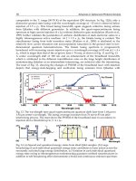
The D, BR, and SR arrivals were described by their peak pressure-squared. Figure 5.13A shows their
spectrum) and is rapidly lost into the bottom. In contrast to the previous experiment (see Appendix 5.A)

Acoustic Remote Sensing of Photosynthetic Activity in Seagrass Beds 81
energy of the D, BR, and SR paths, contained in the leading part, the mean duration increased with the
energy of the MSBR paths and reverberation, contained in the tail (assuming the average power of
ambient noise is constant). As shown later, excess attenuation due to the presence of gas bubbles near
the bottom resulted in a mean-duration decrease.
5.4.4 Non-Photosynthesis-Related Effects
As the objective was to identify the effects of photosynthesis on sound transmission it was equally
important to assess the effects of other environmental — physical and biological — factors.
5.4.4.1 Tide — The amplitude of Mediterranean tide, albeit small, represents a signiÞcant fraction
of the very shallow water depth. The tide modulated the source–receiver and channel geometry, i.e.,
grazing angle at the boundaries and length of all SR paths.
The tide effect is most evident in the time-of-ßight difference between the D and SR paths vs. geotime
(Figure 5.13B). The amplitude, deduced from geometry and depth-average sound speed, is ª40 cm.
Sinusoidal patterns of extreme intensity in the received-signal spectra reveal tide-controlled interference
interference between two continuous waves (CW) with one experiencing an additional 180° phase shift
at the pressure-release surface.
The spectral shape including marked peaks and valleys, e.g., at 0.9 and 3 kHz, relate to the transmitting
FIGURE 5.13 Direct (D), bottom-reßected (BR), and surface-reßected (SR) paths vs. geotime. (A) Normalized energy.
Gray dots and lines: D path; light gray: BR path; black: SR path. The dots are the raw data and the lines connect the half-
hour median averages. (B) Time-of-ßight difference between the SR and D arrivals. Gray dots: raw data; solid line: smoothed
data. LT and HT: low and high tide. R1 data.
–8
–7
–6
–5
–4
–3
–2
–1
0

1
2
Energy (dB)
18 00 06 12 18 00 06 12 18 00 06 12
0.9
0.95
1
Geotime (h)
Time (ms)
A
B
© 2004 by CRC Press LLC
effects between pairs of SBR arrivals (Figure 5.14). These relate to the classical Lloyd’s mirror effect:
sensitivity response of the source (Figure 5.7B), and the overall decrease above 5 kHz is also due to the
82 Handbook of Scaling Methods in Aquatic Ecology: Measurement, Analysis, Simulation
source directivity. At certain frequencies, absolute differences between low- and high-tide spectra were
greater than 10 dB. There is a marked feature in the high-energy band centered about 5 kHz where a
single peak at low tide was split into two peaks at high tide.
The received-signal energy in a narrow frequency band was not suitable to investigate the photo-
synthesis effect since it was too sensitive to the tidal effect. This required integration of the energy over
a wide frequency band so that the time variation was independent of tidal modulation.
5.4.4.2 Sea Surface Motion — Frequency-dependent amplitude and phase ßuctuations of the
received acoustic signal were due to sea-surface roughness or wind speed. These resulted in a partial
loss of correlation across the signal bandwidth, especially in the upper part of the transmitted spectrum.
On September 22, wind started to decrease followed by 2 days of calm sea and low wind speed
conditions. Wind picked up again during the night on September 25.
*
The SR energy, shown in
Figure 5.13A, followed exactly this pattern, being highly correlated with sea-surface roughness observa-
tions. SR energy was even lower than the BR during the rough-sea periods. In Figure 5.10, time

spreading of the 1-ms delayed SR peak due to the generation of micro-multipaths is evident. The
energies of the D and BR paths, which did not interact with the surface, showed no correlation with
the amplitude of wind-generated waves. The time-of-ßight difference (and interference) between these
two arrivals was stable.
During the two calm days, the sea surface acted as a near perfect mirror for most of the transmitted
frequencies. The acoustic variations were then determined principally by changes in the water-column
and seagrass bed conditions. The rapid ßuctuations of the MSBR energy due to sea surface motion
were of smaller amplitude and timescales relative to the variations induced by photosynthesis. They
were averaged out in the half-hour data block processing applied to analyze the main, longer-term,
acoustic variations.
FIGURE 5.14 (Color Þgure follows p. 332.) Received signal spectrum vs. geotime. Normalized energy spectral density
(left scale). The blue-to-red color map corresponds to the range –30 dB to 0 dB. The curves (top scale) are for high tide
(light gray, 0900 hours) and low tide (dark gray, 1530 hours) on September 24, 1999; see Figure 5.13B. The spectra were
computed from the raw acoustic data, i.e., not matched Þltered or equalized, and median-averaged over half-hour periods.
R1 data.
*
Actually, these sea conditions determined the deployment and recovery of the acoustic instruments.
© 2004 by CRC Press LLC
Acoustic Remote Sensing of Photosynthetic Activity in Seagrass Beds 83
5.4.4.3 Water Temperature Profile — The speed of sound in the water column, which depends
on temperature, plays the same role as the index of refraction plays in optics. The path of an acoustic ray
is determined by its initial angle at the source and the sound speed structure. If sound speed is piecewise
linear in depth and range independent, the paths follow either straight line segments or circular arcs.
Sun is the source of sea-surface heating and seaßoor light irradiance. Solar heating modiÞes the water-
sound speed proÞle (SSP) and solar radiation controls the seagrass-oxygen production. Since the two
phenomena, physical and biological, occur contemporaneously, their respective acoustical effects are
not separable on the basis of time delay or timescale differences, and thus deserve special attention.
On September 24, their amplitudes at the sea surface and seaßoor were, respectively, 0.6 and 0.2°C.
During the 0200 to 0900 hours period, the column was perfectly isothermal. Then, a thin mixed layer
and small thermocline developed during the day.

*
The mild, gradual change of SSP (Figure 5.8A) had no noticeable contribution to the main, diurnal
acoustic variations. These were attributed principally to gas production processes as demonstrated later.
A Þrst veriÞcation was to compare acoustic measurements at speciÞc points of the temperature and
dissolved-oxygen time series. For example, on September 24 the negative temperature gradient
w
During the same period, the oxygen concentration at the bottom increased by 0.4 mg/l and then returned
to the same value, C
O
= 6 mg/l (Figure 5.9B). The medium impulse responses observed at the beginning
and end of the period had similar energy time distribution (e.g., the same mean duration 2s
t
ª 18 ms;
Numerical propagation modeling with measured SSP inputs (Figure 5.8A) showed minor differences
in the multipath character between the isospeed and mildly refracting conditions of the experiment.
**
Hence, points in time with different temperature but similar oxygen conditions had nearly identical
acoustic responses. On the other hand, as shown later, substantial acoustic variations were observed
during the isothermal periods at night, which indicated the inßuence of other environmental variables
including the gas void fraction in the seagrass-matte layer.
5.5 Effects of Photosynthesis on Sound Propagation
The foregoing analysis has demonstrated that the variations of broadband acoustic energy, observed on a
day scale, are essentially independent of the tidal cycle and changes in wind and subsurface temperature
conditions. In this section, time series of dissolved oxygen concentration are interpreted together with the
acoustic data to establish a causal relationship between photosynthesis and the diurnal acoustic variations.
5.5.1 Time Variation of Dissolved Oxygen
The water oxygen content was measured near the foliage to monitor the photosynthetic and respiratory
activity (Figure 5.9B). The gas void fraction
***
in the seagrass layer, which inßuences acoustics, was

not directly measured but was obviously related to the concentration of oxygen dissolved in the
surrounding water.
During the two days of calm sea, September 23 and 24, production of air bubbles due to wave action
was sufÞciently small to detect the contribution of photosynthetic oxygen, in spite of the low-productivity
season. The time evolution of the oxygen depth proÞle is correlated with the photosynthesis cycle
(Figure 5.8B). During the rough-sea day, September 22, oxygen concentration near the surface was
substantially higher due to wave action (not shown).
*
Range dependence of the depth proÞle of temperature (sound speed) was negligible because of the short length and sheltered
position of the S-R transect.
**
The medium impulse responses were synthesized from the depth-dependent Green’s function, which was evaluated at a
number of discrete frequencies over the signal frequency range.
***
The volume of gas in bubble form per volume of water.
© 2004 by CRC Press LLC
Small, diurnal temperature (sound speed) variations involved the entire water column (Figure 5.8A).
increased from zero to DT = 0.7°C (Dc = 1.5 m/s) in the period 1100 to 1830 hours (Figure 5.9A).
Figure 5.18B).
84 Handbook of Scaling Methods in Aquatic Ecology: Measurement, Analysis, Simulation
On September 24, the day- and depth-average oxygen concentration was C
O
ª 6 mg/l. After midday,
oxygen increased above the average value up to a maximum of 6.5 mg/l at 1400 hours and then returned
surface was delayed by 2 h with respect to the bottom peak (not shown). During the night, there was a
gradual decrease of bottom oxygen to a minimum of 5.5 mg/l at 0700 hours corresponding to the end
of the respiratory phase.
5.5.2 Effect of Photosynthetic Bubbles on Multipaths
Multipaths refer to sound that is reßected coherently in the specular direction at the channel boundaries
The peaks of the average response are slightly spread in time due to tidal modulation of the pathlengths

and other effects of environmental variability.
Because the sea surface acted as a near-perfect mirror and the water column was nearly isospeed for
most of the observation period, the observed time variations of the multipath character were mostly due
to changes in the acoustic properties near the bottom. Information about photosynthesis was “accumulated”
(“integrated”) in the low-energy MSBR paths that interacted repeatedly with the hard bottom interface
through the seagrass layer.
The most energetic D and SR paths were not inßuenced by the bottom conditions. The received-energy
angles, most of the energy was reßected back into the water column and, as the angle increased, part of
less sensitive to the seagrass and bottom interfaces than the higher-grazing-angle SBR and MSBR paths.
It should be emphasized that the higher-order paths were partially excited at the upper signal frequen-
cies due to the directional response of the source. The EMF processing compensated for ßat spectrum
only on the source axis. Calibration data showed that the transmit voltage response at 60° off axis
all intermediate angles q < 70° was ª3 kHz.
Figure 5.15 compares two snapshots of the medium impulse responses (smoothed log envelope) taken
early morning before the plant respiratory phase and midafternoon during the photosynthesis phase.
Differences in the multipath-reverberation character are noticeable, especially the disappearance in the
afternoon of the main blobs of energy for t < 100 ms.
curve is the difference between a 0.5-h and the 3-night average responses (log envelope). The clustering
FIGURE 5.15 Comparison of a night and a day medium impulse responses. Black: 0410 hours; gray: 1550 hours.
September 24, 1999. The responses were smoothed with a Savitsky–Golay FIR (polynomial) Þlter of degree 2 and frame
size 10 ms. R1 data.
0 50 100 150 200 250
–45
–40
–35
–30
–25
–20
–15
–10

–5
0
Time (ms)
Log magnitude (dB)
04:10
15:50
© 2004 by CRC Press LLC
back to the average value during the remaining part of day (Figure 5.9B). The concentration peak at the
as shown in Figure 5.4. Their overall structure of arrival was resolved in the 4-day average response of
Figure 5.12, where energy peaks are superimposed on the reverberation and ambient noise background.
variations in Figure 5.13A show no evident cyclic behavior relatable to photosynthesis. At low grazing
the energy was transmitted into the bottom (Figure 5.11A). The very low grazing angle BR path was much
decreased by 1 to 13 dB in the frequency range 5 to 16 kHz. The frequency limit for full excitation of
Figure 5.16 shows the overall geotime variability of the acoustic-impulse response. Each overlaid
Acoustic Remote Sensing of Photosynthetic Activity in Seagrass Beds 85
of the responses reveals night and day regimes. Along the time axis, three regions can be isolated with
distinct geotime variability. The regions correspond to the following groups of path and ranges of relative
arrival time and grazing angle:
Subcritical: 2–3 1.5 ms < t < 10 ms q < 40°
Intermediate: 4–12 10 ms < t < 90 ms 40° < q < 70° (5.11)
Near-vertical: 13–• t > 90 ms q > 70°
as determined from the eigenray calculations. The leading part of the response, which includes only two
to three bottom bounces, shows a lesser sensitivity to environmental variability and no diurnal trend.
The tail, which is dominated by reverberation and contaminated by background noise, shows a marked
day–night difference.
The middle part of the response, which includes predominantly reßected and scattered energy in the
specular direction, shows a marked sensitivity to photosynthesis. The contour plot in Figure 5.17 shows
the diurnal variations for that part of the response. At daylight, when gas void fraction increased in the
leaf layer, the energy partly excited into the bottom and partly reradiated to the water column both
decreased owing to scatter and absorption.

The omnidirectional scatter of the intervening bubble layer adds to the directional scatter of the rough
hard bottom. The combined processes redistribute the incident energy in the water column, taking away,
together with the absorption process, a larger portion of the energy transmitted in the specular direction.
The resulting attenuation is expected to be strongly dependent on grazing angle and frequency.
In addition to the attenuation effect, the presence of bubbles in a near-bottom water layer caused ray
refraction. The refraction index of that layer was frequency dependent, as the effect of bubbles on sound
speed depends on the ratio of the excitation frequency to the bubble resonant frequency.
*
When bubble
density increased near the bottom, rays were refracted and reßected at more nearly normal incidence.
It is reasonable to assume that most bubble sizes in the leaf water were much smaller that the bubble
resonant size at the higher frequency of excitation f
2
= 16 kHz, i.e., a radius a = 373 mm at the depth z = 8
m. At frequencies well below the bubble resonances, the sound speed can be determined from the simple
mixture theory. The low frequency, asymptotic value for a gas void fraction U is given by Wood’s equation:
42
FIGURE 5.16 (Color Þgure follows p. 332.) Geotime variability of the medium acoustic-impulse response (log envelope)
in the time-delay range 1 ms to 290 ms. Each line is the difference between a 0.5-hour and the 3-night median averages.
Blue lines: night hours 0700–1930 hours, 4 days; orange lines: day hours, 4 days; green lines: most active photosynthesis
hours 1300–1600 hours, September 24, 1999. Each average response was smoothed with a 10-ms polynomial Þlter. The
vertical lines indicate the time window, which corresponds to intermediate grazing angles. R1 data.
*
This frequency dependence does not exist in bubble-free water where sound speed depends only on temperature, salinity,
and pressure.
© 2004 by CRC Press LLC
86 Handbook of Scaling Methods in Aquatic Ecology: Measurement, Analysis, Simulation
(5.12)
where E
g

= gp
A
and E
w
= r
w
c
w
2
are the bulk moduli of elasticity of gas and water, g = 1.4 is the ratio of
speciÞc heats of gas (air or oxygen), r
g
= 1.43 g l
–1
is the gas density (oxygen), r
w
= 1030 kg m
–3
is
the water density and p
A
= p
A0
+ r
w
gz = 1.81·10
5
Pa is the ambient pressure at a depth z = 8 m. From
Snell’s law, the modiÞed grazing angle on the basalt interface as a function of the void fraction is given by
(5.13)

which is shown in Figure 5.11B for plausible values of the void fraction.
The greater sensitivity of the paths with intermediate grazing angles was due to the reßection loss vs.
angle curve for a basalt half-space (Figure 5.11A) combined with the refraction effect in the seagrass
layer (Figure 5.11B). For an impedance contrast increase due to sound speed (and density) smaller than
bubble-free water, say, for U = 5·10
–5
:
1. The near-horizontal paths at the seagrass interface are refracted but remain in a low-loss region
of the curve.
2. The near-critical paths move to a higher-loss region.
3. Most intermediate paths remain in the high-loss region.
4. The higher ones move to a lower-loss region.
5. The near-vertical paths remain in a medium-loss region.
The net result of (a) the loss redistribution among the paths, (b) their associated number of bottom
bounces, and (c) the attenuation effect explains the shape of the diurnal variations in the middle part of
the medium response envelope (gray line in Figure 5.12 and Figure 5.16).
The plot in Figure 5.11A shows the complexity of the reßection at the composite bottom. The loss
is contoured as a function of angle and frequency. The prediction includes the refraction effect only,
i.e., not the attenuation in the seagrass layer due to scattering and absorption. At the lower frequencies
the loss is similar to the curve of basalt half-space. This is because here the seagrass layer is thin
FIGURE 5.17 (Color Þgure follows p. 332.) Time distribution of multipath energy vs. geotime. The contour lines are
from –4 dB to +1 dB in 1-dB steps. The levels are referenced to the three-night median-average. The displayed time interval
comprises the multipath arrivals of groups 2 through 13. R1 data. See Figure 5.16.
c
EE
UUUEUE
B
gw
gww g
=

()
+-
()
[]
+-
()
[]
12
12 12
11rr
qq
BBww
UcUc() cos ( ( ) / )cos( )=
[]
-1
© 2004 by CRC Press LLC
Acoustic Remote Sensing of Photosynthetic Activity in Seagrass Beds 87
compared to the acoustic wavelength (H = 0.60 m, l = 6.3 m at f
1
= 200 Hz) and therefore acoustically
transparent. The apparent critical angle is seen to decrease with frequency (from 40° to 35° at 1 kHz).
The angle-dependent resonance pattern is evident, with quarter and half-wavelength layer effects
regularly interspersed (on a linear frequency scale).
Figure 5.18A shows the geotime variation of the energy received in one group of multipaths: group 7
with a mean grazing angle of 61°. A remarkable feature is the similarity of shape between the acoustic
and dissolved oxygen time series. The group-7 energy, reversed in the vertical, is overlaid to the plot of
mean duration, 2s
t
= 15 ms (Figure 5.18B) that occurred at 1500 hours, correspond to the maximum
concentration of oxygen near the foliage. Also the maximum of energy coincides with the minimum of

bottom oxygen at 0600 hours. The difference of energy between 0600 and 1500 hours, E = –5 dB,
represents an excess attenuation of ª0.7 dB per bottom bounce. A local minimum of energy was
consistently observed at 0700 hours for the three days (gray arrows in Figure 5.18A) in correspondence
to the oxygen minimum at the end of the respiratory phase. The excess attenuation was attributed to the
concomitant ßows of gas to the rhizomes and roots as discussed in the next section. Similar but smaller
and smoother energy variations were observed for time windows that included a larger number of arrivals
with intermediate grazing angles (not shown).
multipath energy vs. temperature in the upper part of the water column and dissolved oxygen content
near the foliage. In Figure 5.19A, the great scatter of the data pairs indicates no obvious relationship
FIGURE 5.18 Descriptive statistics of the medium acoustic-impulse response vs. geotime. (A) Normalized fractional
energy in the time window 35 to 45 ms, corresponding to the multipath group 7. (B) Mean duration. The gray dots are the
raw data. The circles connected by solid lines are half-hour median averages. The dashed lines are interpreted missing
points. The arrows are explained in the text.
18 00 06 12 18 00 06 12 18 00 06 12
–3
–2
–1
0
1
2
Geotime (h)
Energy (dB)
18 00 06 12 18 00 06 12 18 00 06 12
15
16
17
18
19
20
21

22
Geotime (h)
2σ
t
(ms)
A
B
© 2004 by CRC Press LLC
Figure 5.9B for direct comparison (dashed line). The well-deÞned minima of energy, E = –3 dB, and
Figure 5.19 shows the relationships between the acoustic and environmental measurements: group-7
88 Handbook of Scaling Methods in Aquatic Ecology: Measurement, Analysis, Simulation
between the small temperature (sound speed) gradient and the acoustic energy variations. In Figure 5.19B,
there is a strong (nonlinear) relationship between the oxygen concentration and the received-energy
variations. The energy decreased sharply when the water oxygen content rose above the nominal value
of C
O
= 6 mg/l.
In conclusion, the overall attenuation of the MSBR arrivals during the daylight hours was due to a
near-bottom excess attenuation controlled by photosynthesis.
5.5.3 Effect on Reverberation
Reverberation refers to sound that is scattered away from the specular direction both in and out of the
vertical plane containing the source and receivers. Inhomogeneities within the water body and at the
channel boundaries form discontinuities in the physical properties of the medium and thereby intercept
and reradiate a portion of the acoustic energy incident on them. The sum total of the contribution from
all the scatterers, observed at a receiver distant from the source, is the bistatic reverberation.
the rate of decay. As mentioned earlier, the angle- and frequency-dependent bottom scattering strength
was modiÞed by the seagrass bubble layer. Although the reverberation component was not extracted
from the multipath component, the overall decay time was grossly quantiÞed by the mean duration of
5.5.4
One of the principal features of the ambient noise was its marked time variability. Three major noise

sources were identiÞed: biologics, the wind or waves, and ships and other human-made activities at
moderately close ranges. The diurnal variations in the apparent level of ambient noise were conjectured
to be partly due to photosynthesis.
5.5.4.1 Spectral Characteristics —
level and spectrum observed during the experiment. Abundance and diversity of animals in seagrass
beds are known to increase at night due to immigration of reef Þsh and movement of diurnal planktivores
FIGURE 5.19 Acoustic vs. environmental data. The acoustic data are the energy propagated along intermediate grazing-
(B) Energy vs. dissolved oxygen content near the foliage (z > 8 m). All data points available in both data sets at the same
time (minute) are displayed.
25.2 25.4 25.6 25.8 26
–3
–2
–1
0
1
2
Temperature (°C) [water column]
Energy (dB)
5.4 5.6 5.8 6 6.2 6.4
–3
–2
–1
0
1
2
O
2
(mg/l) [bottom]
Energy (dB)
AB

© 2004 by CRC Press LLC
angle paths (group 7) shown in Figure 5.18A. (A) Energy vs. temperature in the upper part of the water column (z £ 1 m).
As the specularly reßected multipaths, the reverberation was sensitive to photosynthesis. Figure 5.15
Effect on Ambient Noise
and Figure 5.16 show marked differences between night and day in the reverberation character, including
the medium impulse response, which decreased during the daylight hours (Figure 5.18B).
Figure 5.20 shows the diurnal variations of ambient-noise
Acoustic Remote Sensing of Photosynthetic Activity in Seagrass Beds 89
from the water column to sheltering sites beneath the foliage. This behavior was remarkably well
observed during the present experiment from diurnal variations of both ambient noise and volume
scattering features.
The time variation of noise level resembles a square function with characteristic constants of
exponential-like rise and decay times. When darkness approached, the level increased abruptly due to
sounds produced by Þsh migrating into the seagrass bed to feed (Figure 5.20B). During the night, local
biological sounds dominated the natural physical sounds and shipping noise resulting in a 4 to 6 dB
level increase. At sunrise, the apparent level of ambient noise Þrst decreased rapidly and then more
slowly to a minimum before sunset. The rapid decay was due to the diminishing number and intensity
of biological sound sources while the slow decay was attributed to the photosynthesis-driven sound
attenuation characteristics of the plant bubble layer.
The biological origin of sound level increase at night is conÞrmed by a strengthening of the spectral
band centered about 5 kHz (curves in Figure 5.20A). This modiÞed the standard, spectral shape of deep-
sea ambient noise,
40
which is also applicable to shallow water in the absence of biological and human-
made noise. Comparison of night and day averages shows a transition frequency of 1 kHz about which
the power spectral densities varied in an opposite way. Below that frequency, the densities were larger
FIGURE 5.20 (Color Þgure follows p. 332.) Ambient noise vs. geotime. (A) Normalized energy spectral density. The
color map corresponds to the range –30 dB (blue) to 0 dB (red). The spectra were median averaged over half-hour periods.
The overlaid curves are time-mean averages. Dark gray: night hours 1930–0700 hours, 4 days; gray: day hours, 4 days;
light gray: mid-afternoon hours 1400–1600 hours, September 24, 1999. The raw spectra were computed from reverberation-

free data sections of 1-s duration taken before each probe signal was received. Dashed boxes: see text. (B) Normalized
total power. The gray dots are the raw data. The circles connected by solid lines are half-hour median averages. The dashed
lines are interpreted missing points. The data were affected by scuba diving noise during the periods 1440–1520 hours on
September 23 and 1310–1340 hours on September 24 (dashed ellipsis).
© 2004 by CRC Press LLC