HANDBOOK OF SCALING METHODS IN AQUATIC ECOLOGY MEASUREMENT, ANALYSIS, SIMULATION - PART 4 ppsx

229
15
Challenges in the Analysis and Simulation
of Benthic Community Patterns
Mark P. Johnson
CONTENTS
15.1 Empirical and Theoretical Treatments of Spatial Scale in Benthic Ecology 229
15.1.1 Rarity of Spatially Explicit Models for Benthic Systems 230
15.2 Robust Predictions from Spatial Modeling 231
15.3 Comparing Markov Matrix and Cellular Automata Approaches to Analyzing Benthic Data 231
15.3.1 Nonspatial (Point) Transition Matrix Models 233
15.3.2 Spatial Transition Matrix Models 234
15.3.3 Comparison of Empirically DeÞned Alternative Models 235
15.4 Extending the Spatial CA Framework 236
15.5 Conclusions 239
Acknowledgment 240
References 240
15.1 Empirical and Theoretical Treatments of Spatial Scale
in Benthic Ecology
The composition and dynamics of benthic communities reßect the interplay of factors that operate at a
range of scales. Variability at almost every scale of observation is likely to affect benthic species. For
example, hydrodynamic gradients exist from the centimeter scale of the benthic boundary layer to ocean
basin scale circulation patterns. The settlement of benthic species from planktonic life history stages
will reßect both the large-scale and small-scale inßuences on propagule supply. Many benthic species
have limited mobility as adults, so individuals may only interact with other individuals within a relatively
short distance. However, population dynamic processes such as mortality may also be composed of
elements at quite different scales. For example, mortality of barnacles can be caused by both the crowding
effects of neighbors and mobile predators such as whelks or crabs.
Given that there seems no basis for assuming any “correct” scale of observation (Levin, 1992), the
empirical response has been to characterize variability at a number of scales. This form of pattern
identiÞcation can be considered a prerequisite for subsequent studies on process (Underwood et al.,

2000). Many studies of spatial scale have used nested analysis of variance (ANOVA, e.g., Jenkins et al.,
2001; Lindegarth et al., 1995; Morrisey et al., 1992). This may reßect the familiarity of the ANOVA
approach from experimental hypothesis testing in benthic ecology. Indeed, many experimental manipu-
lations also include explicit considerations of scale and scaling effects (Thrush et al., 1997; Fernandes
et al., 1999). Spatial autocorrelation and fractal analyses have also been used to characterize spatial
pattern in benthic systems (Rossi et al., 1992; Underwood and Chapman, 1996; Johnson et al., 1997;
© 2004 by CRC Press LLC
230 Handbook of Scaling Methods in Aquatic Ecology: Measurement, Analysis, Simulation
Maynou et al., 1998; Snover and Commito, 1998; Kostylev and Erlandson, 2001). Although patterns
may have been considered at different times, many studies of spatial scale have taken a snapshot view:
spatial pattern at one point in time has not been mapped onto the spatial pattern at other times. The
snapshot approach restricts further investigation into issues of turnover and dynamics. However, with
the growing interest (Koenig, 1999) in deÞning the spatial scales over which population dynamics are
linked (synchronous), there are likely to be more spatiotemporal studies of benthic populations and
communities in the future. These studies of population synchrony are important as they deÞne the spatial
structure of populations (Koenig, 1999; Johnson, 2001). The degree of synchrony between local popu-
lations has implications for conservation biology. If local populations are asynchronous, then a local
extinction event may be reversed by individuals supplied from another, healthy, population. Large-scale
loss of a species is more likely where local populations are synchronous and no rescue effects occur
(Harrison and Quinn, 1989; Earn et al., 2000).
The inclusion of explicit treatments of spatial scale in much of the empirical research on benthic
systems has not been paralleled by extensive theoretical work on the same systems. Inßuential models
do exist for space-limited benthic systems (Roughgarden et al., 1985; Bence and Nisbet, 1989;
Possingham et al., 1994) and patch dynamics on rocky shores (Paine and Levin, 1981). However,
these models do not have an explicit treatment for space: the variables in the models are not
differentiated on the basis of their relative locations (although see Possingham and Roughgarden,
1990, and Alexander and Roughgarden, 1996, for extensions of the framework to include spatial
population structure along a coastline). Simulations of benthic communities with a one-dimensional
representation of spatial location have been used to look at the development of intertidal zonation
along environmental gradients (Wilson and Nisbet, 1997; Johnson et al., 1998a). Spatially explicit

models of benthic systems on two dimensional lattices have generally shown interactions between
processes at different scales. Local interactions can lead to a large-scale pattern (Burrows and Hawkins,
1998; Wooton, 2001a) and the predictions of spatially explicit and nonspatial models differ (Pascual
and Levin, 1999; Johnson, 2000).
15.1.1 Rarity of Spatially Explicit Models for Benthic Systems
Despite the observation that “space matters” and an explosion of interest in spatial ecology (Tilman and
Kareiva, 1997), there are a number of reasons why spatially explicit models of benthic communities
may be uncommon. The lack of system-speciÞc models partly reßects the manner in which spatial theory
has developed. Spatially explicit models tend to be caricature or generic models that attempt to capture
the essential features of the system (Keeling, 1999). This approach improves the conceptual understand-
ing of systems and allows numerical experiments that would be difÞcult or destructive in a real system
(Keeling, 1999). The use of generic models improves communication between theoreticians as there can
be clarity about techniques and general conclusions without debate on the individual nature of biological
interactions in particular systems.
The rarity of system-speciÞc models can also be explained by considering the problems associated
with an imaginary spatially explicit model for a benthic community. The model is as realistic as
possible, with a number of interacting species inßuenced by stochastic variation in processes such
as recruitment. Simulation output resembles the patterns seen in the real system. However, formal
testing of the model would involve collecting large amounts of detailed spatial data from the Þeld
(independently from that used to derive the model). As the model contains stochastic processes, a
large number of repeated simulations are needed to deÞne the potential behavior of the system. Given
the range of potential outputs that the model may produce, it is difÞcult to envisage how a limited
number of spatial data sets could be used to falsify the model. Both the collection of data and
repeated simulations are time-consuming. More importantly, we are not likely to be interested in the
detailed spatial arrangement of species in the benthic community. Only a subset of model predictions
(such as the mean abundance of a species) is likely to be both of interest to applied research and
testable. Hence the time required to develop a model for a speciÞc system may not be justiÞed in
the end results.
© 2004 by CRC Press LLC
Challenges in the Analysis and Simulation of Benthic Community Patterns 231

15.2 Robust Predictions from Spatial Modeling
There is a tension between the observation that spatial effects can be important and the difÞculties
involved in testing detailed spatially explicit simulations. However, if our understanding of benthic
community patterns is to be addressed, a way of resolving this tension is needed. There have been two
approaches to this problem, which can be loosely classiÞed as theory based and data based.
Theory-based approaches to spatially explicit modeling are extremely diverse and include reaction-
diffusion and partial differential equations. It is difÞcult, however, to construct a mathematically tractable
model that is also applicable to particular ecological systems such as different benthic communities
(Tilman and Kareiva, 1997). In a recent development, researchers have used “pair approximation”
techniques to provide analytically tractable models (Levin and Pacala, 1997; Rand, 1999; see Snyder
and Nisbet, 2000, for a critique and alternative approach). The idea behind pair approximation is that
the equation for a nonspatial process can be extended to a spatial system by using functions that
approximate the average neighborhood structure in a spatial model. Hence, in contrast to a model where
the same equation is repeated at a large number of locations, the small-scale spatial detail is included in a
limited number of equations. The pair approximation approach therefore facilitates investigation of model
behavior more efÞciently than would be the case in a simulation. As yet these models still tend to be
generic, and may thus ignore important features of benthic systems. For example, a common assumption
is that dispersal is a local process (Levin and Pacala, 1997; although see Pascual and Levin, 1999). This
contrasts to the characterization of many benthic populations as open (Roughgarden et al., 1985; Caley et
al., 1996): new recruits may be supplied by sources at some distance from the local population.
In contrast to the development of generic descriptions in the theory-based approach, the data-based
approach involves case studies of speciÞc systems. Ideally, a number of alternative models with different
treatments of space will be tested against Þeld observations. This approach has the advantage that
movement to more complex models is justiÞed only where there are improvements in predictive ability.
The beneÞts of building a sequence of models are further outlined in Hilborn and Mangel (1997).
As it seems impractical to develop a large number of spatially explicit models for different benthic
systems, the challenge in the analysis and simulation of benthic populations is to combine the theory-
based and data-based approaches to produce a set of methodological approaches that can be used to
investigate and contrast different systems. Although this viewpoint is not novel, there remain few
examples of synergy between theoretical and empirical approaches for benthic systems. A notable

exception is the work of Wootton (2001b) on intertidal mussel beds. The approach taken in the Þrst
section below mirrors that of Wootton (2001b) in that multispecies Markov models are used as the
basis for comparing spatial and nonspatial models. A slightly different approach is taken in the second
section, where a more complex model is used to suggest methods for distinguishing between alternative
hypotheses using Þeld data. The analyses presented use a broad interpretation of “benthic” that includes
the rocky intertidal. Rocky shores are generally considered more tractable than sandy or muddy systems.
For example, it is far easier to Þx locations and organisms are generally not subsurface in rocky systems.
On a conceptual level, however, there is nothing to prevent the application of spatial models to sandy
or muddy systems (although the scales of processes such as adult mobility are likely to differ with
increasing mobility of the sediment).
15.3 Comparing Markov Matrix and Cellular Automata Approaches
to Analyzing Benthic Data
What approaches are there available to move beyond generic models and statistical pattern identiÞcation
in the analysis of benthic systems? A Þrst task is to recap on the potential shortcomings of theory-based
and wholly empirical approaches. The generic nature of certain theoretical approaches has been detailed
above. Potential limitations of statistical pattern analysis (e.g., spatial autocorrelations, nested ANOVA)
are restrictions on generalization from results and a lack of sensitivity tests of conclusions. Assessment
© 2004 by CRC Press LLC
232 Handbook of Scaling Methods in Aquatic Ecology: Measurement, Analysis, Simulation
of a pattern, once identiÞed, can be limited to rhetorical arguments about the interaction of processes
at different scales. Follow-up experiments can be difÞcult to design as the alternative, spatially explicit,
hypotheses are not always intuitive. By examining the consequences of different assumptions, models
can extend experimental results to create appropriate hypotheses. Existing techniques for incorporating
Þeld data into a modeling framework include Markov transition matrix models and cellular automata.
Other techniques exist, probably dependent on the ingenuity of the investigator. Markov models and
cellular automata, however, have several advantages. They are well known and relatively simple to apply.
Hence, different investigators can use them and compare results in a common format. Markov models
have the potential for sensitivity testing; they also form an appropriate nonspatial null model for
comparison with data and spatially explicit alternative models. Cellular automata can be used to inves-
tigate neighborhood effects and can be used to identify scaling properties of systems (e.g., power law

relationships in patch geometry; Pascual et al., 2002). Here I emphasize cellular automata as they can
be “twinned” with experimental procedures at the same scale: within shore patches and external forcing
at the grid scale (cf. spatial replication between shores). Other techniques exist for spatial modeling, for
example, applications of geographical information systems (GIS) at the landscape scale. However, GIS
applications are probably closer to statistical pattern analysis in that the scope for sensitivity tests and
experimental investigation of predictions is limited.
Cellular automata (CA) and Markov transition matrix approaches have underlying similarities and yet
they are generally used in completely different ways. Both approaches use a discrete description of time
and state. Temporal dynamics in both frameworks are usually Þrst order: state at time
t + 1 is dependent
on state at time
t. Such transitions may be entirely deterministic or occur with a speciÞed probability.
Where the two approaches differ is that CA includes a discrete representation of space, typically
visualized as a grid of square or hexagonal cells. The cells in the neighborhood of an individual location
on the CA grid inßuence the transition between states at that location from one time step to the next.
Applications of CA usually stress simplicity at the expense of biological realism (Molofsky, 1994; Rand
and Wilson, 1995) but cite speed of computation and heuristic value (Phipps, 1992; Ermentrout and
Edelstein-Keshet, 1993). In comparison, Markov transition matrix models are frequently derived directly
from Þeld data and are used to examine characteristic processes in the observed communities (Horn,
1975; Usher, 1979; Callaway and Davis, 1993; Tanner et al., 1994).
In theory, it is straightforward to reconcile the issues of spatial dependence and empiricism that
transition matrices and CA, respectively, ignore. By constructing a CA using observed local transition
probabilities, it is possible to compare models containing local interactions with nonspatial models.
A problem with this approach is the data requirement needed to parameterize even a simple CA. For
example, a cell in a system with four states and eight neighbors would have 4
8
(65,536) possible
neighborhood conÞgurations. It would be practically impossible to empirically deÞne a transition prob-
ability associated with each neighborhood conÞguration. However, given information about the important
interactions in a system, effort can be concentrated on deÞning a limited number of transitions.

An example of a relatively well studied system is the mosaic of macroalgal (mostly
Fucus spp.)
patches on smooth moderately exposed rocky shores in the northeast Atlantic (Hawkins et al., 1992).
Spatial structure and patch dynamics in this system are thought to be driven by limpet grazing (Hartnoll
and Hawkins, 1985; Johnson et al., 1997). Spatial autocorrelation studies have suggested an algal patch
length scale of approximately 1 m in this system. Time series from a quadrat of similar dimensions to
the patch scale show multiannual variations in algal cover, with limpet densities tending to lag these
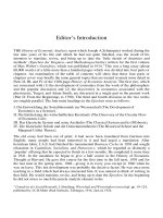
ßuctuations. The conceptual model developed for this system is based on the interaction between limpet
grazing pressure and the recruitment of algae. Limpets are aggregated in clumps on the shore and the
uneven spatial distribution of grazing pressure leads to the formation of new patches of algae in areas
where there are few limpets. The spatial mosaic of algal patches formed by uneven grazing pressure is
in grazing pressure and allows new patches of algae to be generated elsewhere on the shore. Older
patches of algae do not regenerate, possibly because of the increased local density of limpets associated
with them. Hence the shore is patchy, but the locations of patches change, creating the multiannual
ßuctuations seen at the patch scale.
© 2004 by CRC Press LLC
dynamic (Figure 15.1). Adult limpets relocate to established patches of algae. This generates changes
Challenges in the Analysis and Simulation of Benthic Community Patterns 233
The proposed mechanism for the patch mosaics on moderately exposed rocky shores in the northeast
Atlantic implies that the effort in deriving spatial transition rules can be concentrated on deÞning how
they are affected by the local limpet density. By constructing a traditional nonspatial transition matrix
model it is possible to test if the system dynamics are at least a Þrst-order Markov process. Empirically
derived CA rules with and without a local limpet presence can be tested to investigate whether limpets
do actually affect local state transitions. Spatial and nonspatial Markov processes can be compared to
test whether local interactions alter the projected dynamics of the system.
15.3.1 Nonspatial (Point) Transition Matrix Models
Transition matrix models are deÞned by marking out Þxed sites, deÞning states, and recording the
transitions between states in a deÞned time period. In work carried out in the Isle of Man (methods
described more fully in Johnson et al., 1997) the Þxed sites were 0.01 m
2

square “cells” in permanently
marked 5
¥ 5 m quadrats (2500 cells per quadrat) and the time step was 1 year. If a cell contained algae,
a distinction was made between “mature” and “juvenile” cells. A juvenile cell was one where algal frond
lengths did not exceed 0.1 m and reproductive structures were absent. Barnacle cover outside algal
patches was variable. If a cell contained no barnacles at all it was classed as bare rock. Coralline red
algae were generally associated with small rock pools. If the areal cover of coralline red algae exceeded
that of barnacles, a cell was classiÞed as “coralline red.” The presence or absence of adult limpets was
recorded (shell diameter >15 mm) for each of the Þve basic classiÞcation states (barnacle, juvenile,
mature, coralline red, and rock).
Transition matrices take the form:
(15.1)
where
p
jk
is the probability of transition from state k to state j with each time step. Transition probabilities
are derived from a frequency table of state
k to j changes. The frequency of each change from one state
to another is divided by the column total to give the probability of each transition. Transitions are tested
for interdependence (with the null hypothesis being that transitions are independent, i.e., random, and
therefore the process is not Markovian) using a likelihood ratio test, with –2 ln
l compared to c
2
with
(
m –1)
2
degrees of freedom (Usher, 1979):
FIGURE 15.1 Idealized cycle at the patch scale on moderately exposed shores in the northeast Atlantic. Spatial variation
in limpet grazing pressure allows recruitment of juvenile algae to the shore. Patches eventually decay. The aggregation of

limpets in aging patches of algae changes the spatial pattern of grazing pressure, allowing new patches to be formed
elsewhere on the shore.
Barnacles,
no limpets
(b -)
(j -)
(m -)
(b+)
(m+)
Juvenile algae,
no limpets
Mature algae,
no limpets
Mature algae,
limpets
Barnacles,
limpets
A =
Ê
Ë
Á
Á
Á
Á
Á
Á
ˆ
¯
˜
˜

˜
˜
˜
˜
ppp p
ppp p
ppp p
ppp p
n
n
n
nn n nn
11 12 13 1
21 22 23 2
31 32 33 3
123
L
L
L
MMMMM
L
© 2004 by CRC Press LLC
234 Handbook of Scaling Methods in Aquatic Ecology: Measurement, Analysis, Simulation
(15.2)
where
(15.3)
n
jk
= number of transitions from state k to j in the original data matrix
p

jk
= probability of transition from state k to j
p
j
= sum of transition probabilities to state j
m
= order of the transition matrix (number of rows)
The sum effect of all transitions over a time step is found by the multiplication:
(15.4)
where x
(t)
is a column vector containing frequencies of separate cell state at time t. With transition
matrices, repeated multiplication by
A generally causes the community composition to asymptotically
approach a stable state distribution deÞned by the right eigenvector of
A (Tanner et al., 1994).
The temporal scales of processes can be investigated from metrics derived from transition matrices.
For example, the rate of convergence to a stable stage structure is governed by the damping ratio,
r
(Tanner et al., 1994; Caswell, 2001):
(15.5)
where
l
j
is an eigenvalue of the transition matrix. As matrix columns sum to one, the Þrst eigenvalue
is always one. A convergence timescale is given by
t
x
, the time taken for the contribution of the Þrst
eigenvalue to be

x times as great as the contribution from the second eigenvalue (Caswell, 2001):
(15.6)
15.3.2 Spatial Transition Matrix Models
Maps of adjacent 0.01 m
2
cells allow spatial transition rules to be deÞned. The effect of limpets on the
transitions occurring in their neighborhood can be tested by deriving two separate transition matrices:
one for transitions when limpets were present in at least one of the neighboring eight cells and one
matrix for cell transitions occurring in the absence of limpets in surrounding cells. The signiÞcance of
differences between “local limpets” and “no local limpets” transition matrices can be examined using
(Usher, 1979; Tanner et al., 1994):
(15.7)
where
L = number of transition matrices associated with limpet grazing effects (= 2)
n
jk
(L)= number of k to j transitions recorded for matrix L
p
jk
(L)= transition probability from k to j in matrix L
p
jk
= transition probability from k to j if L matrices are pooled
The likelihood ratio is compared to
c
2
with m(m – 1)(L – 1) degrees of freedom and a null hypothesis
that there is no difference between matrices dependent on the presence or absence of limpets in the eight
cell neighborhood.
-=

Ê
Ë
Á
ˆ
¯
˜
==
ÂÂ
22
11
ln lnl n
p
p
jk
jk
j
k
m
j
m
p
n
n
j
jk
jk
k
m
j
m

k
m
=
==
=
ÂÂ
Â
11
1
Ax x
t
t1
()
+
()
=
rl l=
12
/
tx
x
= ln( ) / ln( )r
-=
Ê
Ë
Á
ˆ
¯
˜
===

ÂÂÂ
22
111
ln ( )ln
()
l nL
pL
p
jk
jk
jk
L
L
k
m
j
m
© 2004 by CRC Press LLC
Challenges in the Analysis and Simulation of Benthic Community Patterns 235
It is not possible to iterate the spatial model using matrix multiplication as the choice of transition
probability is dependent on local conditions. Spatial transition matrices were therefore investigated using
CA simulations. These simulations were based on 50
¥ 50 square cell grids with periodic boundary
conditions (cells on one edge of the grid are considered to be neighbors to cells on the opposite edge of
the grid). As the CA rules are derived empirically from counts of 0.01 m
2
cells, spatial simulations represent
an area of 25 m
2
. Cell state transitions at each time step were based on probabilities drawn from a matrix

chosen according to the neighborhood state (“local limpets” or “no local limpets”). Simulations were
stochastic as random numbers were used to generate cell state transitions based on the probabilities in the
appropriate matrix (the spatial model was what is sometimes referred to as a “probabilistic CA”).
15.3.3 Comparison of Empirically Defined Alternative Models
Point and spatial transition matrices were derived for three separate 25 m
2
quadrats at different sites in
the Isle of Man (hereafter referred to as sites
a, b, and c). At each site, likelihood ratio tests supported
the application of Markov matrices to the observed transitions (Equation 15.2,
p < 0.001 in all cases).
Hence the matrices contain information about a nonrandom process of transitions at each site.
An example point transition matrix is shown in Table 15.1. The pattern of transitions reßects parts of
the patch cycle proposed by Hartnoll and Hawkins (1985). For example, the majority of barnacle-classiÞed
cells became occupied by algae. Most cells classed as juvenile algae were recorded as mature algae in the
following year. The predicted dynamics rapidly approached equilibrium, with convergence time scales
(
t
10
) of 4.17, 1.51, and 1.23 years for sites a, b, and c, respectively. This implies a high degree of resilience
at two of the sites with recovery to the equilibrium state within 2 years of a perturbation. It is not clear
what features make site
a recover more slowly than the other sites. One possibility currently under
investigation is that variation in dynamics reßects differences in surface topography.
The spatial transition matrices for the “no local limpets” and “local limpet” cases were signiÞcantly
different at all three sites (Equation 15.7,
p < 0.05). This supports the hypothesis (Hartnoll and Hawkins,
1985) that the spatial pattern of limpet grazing affects interactions on the shore. There was some variation
between sites, but the transition frequencies reßected the inßuences of limpets on transitions to algal
cover. For example, at the site with the largest difference between matrices, 63% of all transitions were

to algal occupied states in the “no local limpets” matrix compared to 53% in the “local limpets” case.
As has been shown elsewhere (Wootton, 2001b), predictions of the matrix models Þt the observed state
G tests show that the Þt of the models is closer than would be expected for randomly generated frequencies,
The discrepancy between predicted and observed frequencies was generally not reduced by using a
spatial rather than a point model. In addition, the predictions of spatial and point models were not
signiÞcantly different for site
c. Despite the detection of spatial effects associated with limpets, the
increase in model complexity from point to spatial models was not justiÞed by a better Þt to the data.
TABLE 15.1
Matrix of Transition Probabilities for Quadrat a Surveyed in the Isle of Man
b+ b– j+ j– m+ m– cr+ cr–
b+ 0.024 0.036 0.000 0.015 0.028 0.010 0.100 0.039
b– 0.040 0.105 0.021 0.024 0.028 0.030 0.100 0.078
j+ 0.079 0.042 0.021 0.039 0.056 0.035 0.050 0.024
j– 0.333 0.224 0.128 0.119 0.139 0.055 0.050 0.083
m+ 0.095 0.072 0.149 0.124 0.250 0.199 0.000 0.044
m– 0.397 0.468 0.670 0.671 0.500 0.662 0.200 0.150
cr+ 0.000 0.004 0.000 0.003 0.000 0.005 0.050 0.044
cr– 0.032 0.048 0.011 0.006 0.000 0.005 0.450 0.539
Note: Cells are classiÞed as barnacle occupied (b), juvenile Fucus (j), mature Fucus (m),
and coralline red algae (cr). Bare rock was not recorded in cells at this site.
+ or – modiÞers indicate the presence or absence of limpets in the cells.
© 2004 by CRC Press LLC
frequencies reasonably well (explaining between 45 and 97% of the variation in frequencies; Figure 15.2).
but that there were still departures between model predictions and observed frequencies (Table 15.2).
236 Handbook of Scaling Methods in Aquatic Ecology: Measurement, Analysis, Simulation
The spatial model may still have some heuristic value if it generates a dynamic pattern of states in
simulations. Techniques for investigating spatiotemporal pattern include calculating correlations between
sites at different distances from each other (Koenig, 1999). An alternative approach used in scaling
investigations of spatial models (De Roos et al., 1991; Rand, 1994; Rand and Wilson, 1995) is to compare

the dynamics of cell frequencies in “windows” of different sizes on the simulation grid. For any probabilistic
CA, cell state frequencies will ßuctuate with time. The standard deviation of a time series taken from a
window of
L ¥ L grid cells will decrease with increasing L (tending to zero at very large window sizes).
For a stochastic process, the reduction in standard deviation with window size will generally be proportional
to 1/
L (Keeling, 1999). However, if a model contains coherent patch structures, there will be deviations
from the 1/
L line predicted for a stochastic process. If the patches are long-lived structures with respect to
the time series, then standard deviations taken from windows smaller or equal to the patch scale will be
less variable than expected. The expected scaling behavior is seen in time series drawn from a probabilistic
version of the point model (transitions occur to populations of
L ¥ L cells with probabilities drawn from
and window size was the same in probabilistic point and spatial models (ANCOVA,
p no difference between
slopes > 0.5). Hence there is no evidence that patch structures are formed at any scale in the spatial model.
15.4 Extending the Spatial CA Framework
The derivation of a spatial matrix model demonstrated that the local density of limpets affected the
transitions between states on the shore. However, the empirically derived CA failed to generate spatial
FIGURE 15.2 Comparison of observed and predicted cell state frequencies in 25 m
2
sampling quadrats. Observed frequencies
are the average of separate annual samples. Predicted frequencies are from point or spatial transition matrix models.
0
200
400
600
800
1000
1200

1400
1600
Observed
Point
Spatial
0
100
200
300
400
500
600
State frequency (0.01 m
2
cells occupied)
0
200
400
600
800
1000
Barnacles +
Barnacles -
Juveniles +
Juveniles -
Mature +
Mature -
Coralline +
Coralline -
Rock +

Rock -
Site a
Site b
Site c
© 2004 by CRC Press LLC
the nonspatial matrix for site a; Figure 15.3). The relationship between standard deviation of time series
Challenges in the Analysis and Simulation of Benthic Community Patterns 237
pattern or improve model predictions of state frequencies when compared to a nonspatial model. Wootton
(2001a) in a study of intertidal mussel beds also found that empirically derived CA simulations with
local interactions (but without locally propagated disturbances) did not produce patterning. The absence
of spatial pattern in the CA models may reßect that spatial structures are sensitive to the stochastic
nature of transitions between states (Rohani et al., 1997). The spatial transition rules for the Fucus
mosaic and mussel bed were deÞned from Þeld data. This implies that it is not possible to scale up from
observations at small scales to patterns at large scales. There are, however, two reasons this conclusion
may be premature. It may be that the CA framework is too crude a method to characterize the local
interactions in the intertidal. The CA models also did not include “historical” effects, despite the
TABLE 15.2
Comparisons between the Observed Frequencies of Different States,
the Predictions of Point and Spatial Models, and Community Frequencies
Generated Randomly
Observed Point Model Spatial Model
Site a
Point model 2005.41
Spatial model 1883.29 22.17
Random 3533.15 6120.27 5907.50
Site b
Point model 753.58
Spatial model 784.86 39.36
Random 6350.90 5576.49 4895.45
Site c

Point model 42.01
Spatial model 56.41 4.77
Random 3166.67 3826.65 3766.11
Note: G tests (Sokal and Rohlf, 1995) are used as measures of goodness of Þt
(Wootton, 2001b). Scores for the random model communities are averages of
250 independently generated tests. Lower G test values imply a better match
between the frequencies being compared. Numbers in bold indicate signiÞcant
differences between the frequencies being compared.
FIGURE 15.3 Standard deviation of mature algal frequencies in time series collected at different spatial scales. Observation
window length scales range from 4 to 256 cells. The common slope is a statistically signiÞcant regression passing through
the origin.
1/(observation window length scale)
0.00 0.05 0.10 0.15 0.20 0.25 0.30
Standard deviation of time series for
frequency of mature algal state
0.00
0.02
0.04
0.06
0.08
0.10
0.12
Stochastic spatial model
Stochastic nonspatial model
Common slope
© 2004 by CRC Press LLC
238 Handbook of Scaling Methods in Aquatic Ecology: Measurement, Analysis, Simulation
observation that history can intensify local interactions in probabilistic CA, leading to pattern formation
(Hendry and McGlade, 1995).
In the context of Markov transition matrices, historical effects are modiÞcations to the transition

probabilities based on the state of the system at lags exceeding one time step (models include second
and higher order processes, Tanner et al., 1996). Hence the age of particular states can affect their
transition probabilities. For example, not all mussel beds are equivalent. Waves are more likely to remove
old, multilayered beds (Wootton, 2001a). In the Fucus mosaic, patches of algae persist for 5 years before
they break down (Southward, 1956). Tanner et al. (1996) demonstrated that historical effects could be
detected in coral communities, although these effects did not affect overall community composition in
comparison to Þrst-order models.
Incorporating a more sophisticated representation of local grazing interactions and historical effects
into CA simulations requires a framework variously known as mobile cellular automata, lattice gas
model, or artiÞcial ecology (Ermentrout and Edelstein-Keshet, 1993; Keeling, 1999). Time, space, and
state are still discrete, but the artiÞcial ecology formulation allows simulated organisms to move around
the grid. This is a more ßexible method of representing aggregations of mobile organisms than a
conventional CA.
An artiÞcial ecology for the Fucus patch mosaic can be based on the spatial effect of individual limpets
on the probability that new patches of algae will be formed. This relationship can be deÞned from maps
of limpet and algal location. The maps previously used for transition matrices have a minimum spatial
scale below the average distance that limpets forage from their semipermanent home scar (0.4 m; Hartnoll
and Wright, 1977). Hence the grazing effects should extend over several 0.01 m
2
cells. Stepwise logistic
regression using increasing distances from the target cell was used to deÞne the strength and the range
of limpet effects on the probability of a cell containing juvenile algae (Johnson et al., 1997). This
information was then used to simulate the Fucus mosaic in a 50 ¥ 50 cell grid, equivalent to the scale of
the maps made in the Þeld. Each time step the distribution of limpets deÞned the probability of juvenile
Fucus establishing in any unoccupied cell on the grid. As on the shore, limpets potentially relocated to
new home scars each year, creating a dynamic pattern of grazing pressure. Simulations of this artiÞcial
ecology created realistic mosaic patterns (Figure 15.4). A fuller description of the model, including
investigation of the roles of limpet movement and habitat preferences is given in Johnson et al. (1998b).
An advantage of the empirically deÞned rules for the artiÞcial ecology is that the scales in the
simulations are clearly deÞned. This facilitates more demanding confrontations with data than is possible

with more generic spatial models. For example, the spatial autocorrelation produced in simulations gives
FIGURE 15.4 Screen grab of simulation output from the artiÞcial ecology of the limpet–Fucus mosaic. The spatial plots
show (A) Fucus distribution (white–empty, gray–juvenile, black–mature) and (B) limpet occupancy (white–empty, gray–one
limpet, black–more than one limpet). The time series (500 time steps) of algal cover (C) shows records from the patch
scale (black line) and the grid scale (gray line).
© 2004 by CRC Press LLC
Challenges in the Analysis and Simulation of Benthic Community Patterns 239
a patch length scale of approximately 0.4 m, compared to a patch scale of 0.8 m for the same location
in the Þeld. The better deÞnition of patches in the Þeld may reßect heterogeneity in limpet grazing
efÞciency or algal recruitment probability associated with small-scale topographic features. These features
could be investigated further by looking at local deviations (residuals) from the Þtted regression of
recruitment probability to grazer density (see Sokal et al., 1998, for a related approach to deÞning
structures with local spatial autocorrelation).
Reßection on scale in the artiÞcial ecology draws attention to the lack of scaling in the original time
series. Although records of ßuctuation in Fucus cover and limpet abundance exist for a period of over
20 years, the spatial scale of observations is limited to a 2 m
2
permanent quadrat. From a Þxed scale of
observation, it is not clear whether the small-scale process of limpet grazing really drives the ßuctuations
in algal cover or whether the ßuctuations reßect larger-scale processes such as interannual variability in
recruitment success across the entire shore (Gunnill, 1980; Lively et al., 1993). These alternatives can
be tested by looking at the correlation between small and large scales. Where local grazing processes
contrast, if the recruitment of Fucus is unpredictable at large scales, the dynamics at the patch scale and
the large scale become correlated (Figure 15.5). This observation suggested a novel way of using a
photographic time series of the entire shore in the Isle of Man to examine the inßuence of small-scale
processes on Fucus abundance (Johnson et al., 1998b). A consistent ranking of the photographs was
produced after presenting them in random order to seven different observers. The correlation between
this ranking and the abundance of Fucus in records from the 2 m
2
quadrat was low (0.237, p > 0.5).

Hence Þeld observations suggest that local processes are important in the temporal dynamics of the
Fucus mosaic on rocky shores in the northeast Atlantic.
15.5 Conclusions
Research on the limpet–Fucus mosaic and mussel beds (Wootton, 2001b) suggests that it is possible to
combine empirical and theoretical approaches directly to improve the understanding of processes in
benthic communities. Empirical description of model rules facilitates model testing, while the models
themselves can be used to derive new ways of testing Þeld data. The tools applied here have different
strengths and weaknesses, but they can generally be applied to analysis of the same data set. Contrasts
between the predictions of the different methods may provide a fuller understanding of any community
than application of a single approach.
FIGURE 15.5 Correlations between Fucus abundance at patch and grid spatial scales with increasing levels of variability
in grid scale Fucus recruitment probability. Time series were 500 time steps long with the Þrst 50 time steps excluded to
remove transient behavior.
Interannual variance in
Fucus
recruitment probability
0.00 0.01 0.02 0.03
Correlation between time series at patch
and grid scales
-0.25
0.00
0.25
0.50
0.75
1.00
© 2004 by CRC Press LLC
are important, the patches cycle independently of Fucus abundance at the large scale (Figure 15.2C). In
240 Handbook of Scaling Methods in Aquatic Ecology: Measurement, Analysis, Simulation
Markov transition matrices appear to produce reasonable Þrst approximations of community composi-
tion. This may reßect the relatively open nature of many benthic communities. The transition rate to a

certain state (say, mussel occupied) may not be affected by the number of sites already occupied by
mussels as the larvae come from elsewhere (the population is open). Under these circumstances, the
frequency-invariant nature of transition probabilities may not be an issue. Further research on Markov
models is needed to characterize the features that would result in inaccurate projections of community
composition. Algorithms are needed for parsimonious selection of community states in the matrices as
well as investigations of spatial grain (the optimal size of the “cells” in models). The sensitivity of
communities to particular species transitions is an interesting area. Tanner et al. (1994) present a
sensitivity analysis that may be technically invalid: perturbations to transition probabilities cannot be
examined independently of one another due to the constraint on column totals in the transition matrix
to sum to 1. Wootton (2001b) suggests an alternative method of sensitivity analysis when looking at the
loss of species from a community. The temporal scaling of community dynamics provided by the
convergence timescales may be a useful way of classifying community resilience to perturbations. It
would be interesting to test this approach using data from the time series that exist from experimental
perturbations of rocky shore communities (e.g., Dye, 1998).
The spatial transition matrix models appear to offer fewer insights on community pattern. Despite the
demonstration of a spatial component to transition probabilities based on the presence or absence of
limpets in adjoining cells, there were no improvements in predictive power in comparison to nonspatial
models. In addition the CA approach did not generate spatial pattern. However, spatial transition matrix
models are relatively easy to derive as an alternative to point models. The two matrices derived are a
subset of a very large number of possible spatial transition rules. Even if the rules do not generate
pattern, they can be used as part of a number of methods of investigating structuring processes in
communities (e.g., Law et al., 1997), although some techniques may be restricted (Freckleton and
Watkinson, 2000) to species with limited dispersal of propagules. One area where simpler spatial
transition matrix models may be appropriate is in communities where space-occupying individuals or
colonies grow out horizontally so that effects on neighbors are strong. Encrusting communities of groups
such as bryozoans (Barnes and Dick, 2000) could be an example of this.
The most ßexible approach to modeling communities is to use an artiÞcial ecology. There are dangers
of producing a sophisticated “realistic” model that is intuitively satisfying yet fails to provide insights on
the dynamics and spatial scales of real communities. A potential check on this is to embed empirically
deÞned rules and scales within the model. Hence it should be clear where to look for any scaling behavior

or patterns derived in the model. A potential restriction on wider application of these techniques is that
benthic ecologists have tended not to collect data repeatedly on regularly spaced grids. However, repeated
data collection at the same sites can be a powerful technique for identifying pattern and process (Bouma
et al., 2001). It has been suggested that regularly spaced samples can complement the more common
ANOVA-based hierarchical techniques (Underwood and Chapman, 1996). If use of both survey approaches
becomes more common, this will increase the opportunities to investigate scaling in empirically based
models of benthic communities.
Acknowledgment
Steve Hawkins and Mike Burrows provided fruitful discussion on aspects of this work.
References
Alexander, S.E. and Roughgarden, J., Larval transport and population dynamics of intertidal barnacles: a coupled
benthic/oceanic model, Ecol. Monogr., 66, 259, 1996.
Barnes, D.K.A. and Dick, M.H., Overgrowth competition in encrusting bryozoan assemblages of the intertidal
and infralittoral zones of Alaska, Mar. Biol., 136, 813, 2000.
© 2004 by CRC Press LLC
Challenges in the Analysis and Simulation of Benthic Community Patterns 241
Bence, J.R. and Nisbet, R.M., Space-limited recruitment in open systems: the importance of time delays,
Ecology, 70, 1434, 1989.
Bouma, H., de Vries, P.P., Duiker, J.M.C., Herman, P.M.J., and Wolff, W.J., Migration of the bivalve Macoma
balthica on a highly dynamic tidal ßat in the Westerschelde estuary, The Netherlands, Mar. Ecol. Prog.
Ser., 224, 157, 2001.
Burrows, M.T. and Hawkins, S.J., Modelling patch dynamics on rocky shores using deterministic cellular
automata, Mar. Ecol. Prog. Ser., 167, 1, 1998.
Caley, M.J., Carr, M.H., Hixon, M.A., Hughes, T.P., Jones, G.P., and Menge, B.A., Recruitment and the local
dynamics of open marine populations, Annu. Rev. Ecol. Syst., 27, 477, 1996.
Callaway, R.M. and Davis, F.W., Vegetation dynamics, Þre and the physical environment in coastal central
California, Ecology, 74, 1567, 1993.
Caswell, H., Matrix Population Models, 2nd ed., Sinauer Associates, Sunderland, MA, 2001, chap. 4.
De Roos, A.M., McCauley, E., and Wilson, W.G.,. Mobility versus density-limited predator-prey dynamics
on different spatial scales, Proc. R. Soc. Lond. B, 246, 117, 1991.

Dye, A.H., Dynamics of rocky intertidal communities: analyses of long time series from South African shores,
Estuarine Coastal Shelf Sci., 46, 287, 1998.
Earn, D.J.D., Levin, S.A., and Rohani, P., Coherence and conservation, Science, 290, 1360, 2000.
Ermentrout, G.B. and Edelstein-Keshet, L., Cellular automata approaches to biological modelling, J. Theor.
Biol., 160, 97, 1993.
Fernandes, T.F., Huxham, M., and Piper, S.R., Predator caging experiments: a test of the importance of scale,
J. Exp. Mar. Biol. Ecol., 241, 137, 1999.
Freckleton, R.P. and Watkinson, A.R., On detecting and measuring competition in spatially structured plant
communities, Ecol. Lett., 3, 423, 2000.
Gunnill, F.C., Recruitment and standing stocks in populations of one green alga and Þve brown algae in the
intertidal zone near La Jolla, California during 1973–1977, Mar. Ecol. Prog. Ser., 3, 231, 1980.
Harrison, S. and Quinn, J.F., Correlated environments and the persistence of metapopulations, Oikos, 56,
293, 1989.
Hartnoll, R.G. and Hawkins, S.J., Patchiness and ßuctuations on moderately exposed rocky shores, Ophelia,
24, 53, 1985.
Hartnoll, R.G. and Wright, J.R., Foraging movements and homing in the limpet Patella vulgata L., Anim.
Behav., 25, 806, 1977.
Hawkins, S.J., Hartnoll, R.G., Kain(Jones), J.M., and Norton, T.A., Plant-animal interactions on hard substrata
in the north-east Atlantic, in Plant-Animal Interactions in the Marine Benthos, John, D.M., Hawkins, S.J.,
and Price, J.H., Eds., Systematics Association Special Vol. 46, Clarendon Press, Oxford, U.K., 1992,
1–32.
Hendry, R.J. and McGlade, J.M., The role of memory in ecological systems, Proc. R. Soc. Lond. B, 259,
153, 1995.
Hilborn, R. and Mangel, M., The Ecological Detective, Princeton University Press, Princeton, NJ, 1997, chap. 1.
Horn, H.S., Forest succession, Sci. Am., 232, 90, 1975.
Jenkins, S.R., Aberg, P., Cervin, G., Coleman, R.A., Delany, J., Hawkins, S.J., Hyder, K., Myers, A.A.,
Paula, J., Power, A.M., Range, P., and Hartnoll, R.G., Population dynamics of the intertidal barnacle
Semibalanus balanoides at three European locations: spatial scales of variability, Mar. Ecol. Prog.
Ser., 217, 207, 2001.
Johnson, M., A re-evaluation of density dependent population cycles in open systems, Am. Nat., 155, 36, 2000.

Johnson, M.P., Metapopulation dynamics of Tigriopus brevicornis (Harpacticoida) in intertidal rock pools.
Mar. Ecol. Prog. Ser., 211, 215, 2001.
Johnson, M.P., Burrows, M.T., Hartnoll, R.G., and Hawkins, S.J., Spatial structure on moderately exposed
rocky shores: patch scales and the interactions between limpets and algae, Mar. Ecol. Prog. Ser., 160,
209, 1997.
Johnson, M.P., Hawkins, S.J., Hartnoll, R.G., and Norton, T.A., The establishment of fucoid zonation on algal
dominated rocky shores: hypotheses derived from a simulation model, Functional Ecol., 12, 259, 1998a.
Johnson, M.P., Burrows, M.T., and Hawkins, S.J., Individual based simulations of the direct and indirect
effects of limpets on a rocky shore Fucus mosaic, Mar. Ecol. Prog. Ser., 169, 179, 1998b.
Keeling, M., Spatial models of interacting populations, in Advanced Ecological Theory, McGlade, J., Ed.,
Blackwell Science, Oxford, U.K., 1999, chap. 4.
© 2004 by CRC Press LLC
242 Handbook of Scaling Methods in Aquatic Ecology: Measurement, Analysis, Simulation
Koenig, W.D., Spatial autocorrelation of ecological phenomena, Trends Ecol. Evol., 14, 22, 1999.
Kostylev, V. and Erlandson, J., A fractal approach for detecting spatial hierarchy and structure on mussel beds,
J. Mar. Biol., 139, 497, 2001.
Law, R., Herben, T., and Dieckmann, U., Non-manipulative estimates of competition coefÞcients in a montane
grassland community, J. Ecol., 85, 505, 1997.
Levin, S.A., The problem of pattern and scale in ecology, Ecology, 73, 1943, 1992.
Levin, S.A. and Pacala, S.W., Theories of simpliÞcation and scaling of spatially distributed processes, in Spatial
Ecology, Tilman, D. and Kareiva, P., Eds., Princeton University Press, Princeton, NJ, 1997, chap. 12.
Lindegarth, M., Andre, C., and Jonsson, P.R., Analysis of the spatial variability in abundance and age structure
of two infaunal bivalves, Cerastoderma edule and C. lamarcki, using hierarchical sampling programmes,
Mar. Ecol. Prog. Ser., 116, 85, 1995.
Lively, C.M., Raimondi, P.T., and Delph, L.F., Intertidal community structure: space-time interactions in the
Northern Gulf of California, Ecology, 74, 162, 1993.
Maynou, F.X., Sarda, F., and Conan, G.Y., Assessment of the spatial structure and biomass evaluation of
Nephrops norvegicas (L.) populations in the northwestern Mediterranean by geostatistics, ICES J. Mar.
Sci., 55, 102, 1998.
Molofsky, J., Population dynamics and pattern formation in theoretical populations, Ecology, 75, 30, 1994.

Morrisey, D.J., Howitt, L., Underwood, A.J., and Stark, J.S., Spatial variation in soft sediment benthos, Mar.
Ecol. Prog. Ser., 81, 197, 1992.
Paine, R.T. and Levin, S.A., Intertidal landscapes: disturbance and the dynamics of pattern, Ecol. Monogr.,
51, 145, 1981.
Pascual, M. and Levin, S.A., Spatial scaling in a benthic population model with density-dependent disturbance,
Theor. Popul. Biol., 56, 106, 1999.
Pascual, M., Roy, M., Guichard, F., and Flierl, G., Cluster size distributions: signatures of self-organization
in spatial ecologies, Philos. Trans. R. Soc. Lond. B, 357, 657, 2002.
Phipps, M.J., From local to global: the lesson of cellular automata, in Individual-Based Models and Approaches
in Ecology: Populations, Communities and Ecosystems, DeAngelis, D.L. and Gross, L.J., Eds., Chapman
& Hall, London, 1992, 165–187.
Possingham, H.P. and Roughgarden, J., Spatial population dynamics of a marine organism with a complex
life cycle, Ecology, 71, 973, 1990.
Possingham, H., Tuljapurkar, S.D., Roughgarden, J., and Wilks, M., Population cycling in space limited
organisms subject to density dependent predation, Am. Nat., 143, 563, 1994.
Rand, D.A., Measuring and characterizing spatial patterns, dynamics and chaos in spatially extended dynamical
systems and ecologies, Philos. Trans. R. Soc. Lond. A, 348, 498, 1994.
Rand, D., Correlation equations and pair approximations for spatial ecologies, in Advanced Ecological Theory,
Mcglade, J., Ed., Blackwell Science, Oxford, U.K., 1999, chap. 5.
Rand, D.A. and Wilson, H.B., Using spatio-temporal chaos and intermediate-scale determinism to quantify
spatially extended ecosystems, Proc. R. Soc. Lond. B, 259, 111, 1995.
Rohani, P., Lewis, T.J., Grünbaum, D., and Ruxton, G.D., Spatial self-organization in ecology: pretty patterns
or robust reality? Trends. Ecol. Evol., 12, 70, 1997.
Rossi, R.E., Mulla, D.J., Journel, A.G., and Franz, E.H., Geostatistical tools for modeling and interpreting
ecological spatial dependence, Ecol. Monogr., 62, 277, 1992.
Roughgarden, J., Iwasa, Y., and Baxter, C., Demographic theory for an open marine population with space-
limited recruitment, Ecology, 66, 54, 1985.
Snover, M.L. and Commito, J.A., The fractal geometry of Mytilus edulis L. spatial distribution in a soft-bottom
system, J. Exp. Mar. Biol. Ecol., 223, 53, 1998.
Snyder, R.E. and Nisbet, R.M., Spatial structure and ßuctuations in the contact process and related models,

Bull. Math. Biol., 62, 959, 2000.
Sokal, R.R. and Rohlf, F.J., Biometry, 3rd ed., W.H. Freeman, New York, 1996, chap. 17.
Sokal, R.R., Oden, N.L., and Thomson, B.A., Local spatial autocorrelation in biological variables, Biol. J. Linn.
Soc., 65, 41, 1998.
Southward, A.J., The population balance between limpets and seaweeds on wave beaten rocky shores, Annu.
Rep. Mar. Biol. Stat. Port. Erin., 68, 20, 1956.
Tanner, J.E., Hughes, T.P., and Connell, J.H., Species coexistence, keystone species and succession: a sensitivity
analysis, Ecology, 75, 2204, 1994.
© 2004 by CRC Press LLC
Challenges in the Analysis and Simulation of Benthic Community Patterns 243
Tanner, J.E., Hughes, T.P., and Connell, J.H., The role of history in community dynamics: a modelling
approach, Ecology, 77, 108, 1996.
Thrush, S.F., Cummings, V.J., Dayton, P.K., Ford, R., Grant, J., Hewitt, J.E., Hines, A.H., Lawrie, S.M.,
Pridmore, R.D., Legendre, P., McArdle, B.H., Schneider, D.C., Turner, S.J., Whitlatch, R.B., and
Wilkinson, M.R., Matching the outcome of small-scale density manipulation experiments with larger
scale patterns: an example of bivalve adult/juvenile interactions, J. Exp. Mar. Biol. Ecol., 216, 153, 1997.
Tilman, D. and Kareiva, P., Spatial Ecology, Princeton University Press, Princeton, NJ, 1997.
Underwood, A.J. and Chapman, M.G., Scales of spatial patterns of distribution of intertidal invertebrates,
Oecologia, 107, 212, 1996.
Underwood, A.J., Chapman, M.G., and Connell, S.D., Observations in ecology: you can’t make progress on
processes without understanding the patterns, J. Exp. Mar. Biol. Ecol., 250, 97, 2000.
Usher, M.B., Markovian approaches to ecological succession, J. Anim. Ecol., 48, 413, 1979.
Wilson, W.G. and Nisbet, R.M., Cooperation and competition along smooth environmental gradients, Ecology,
78, 2004, 1997.
Wootton, J.T., Local interactions predict large-scale pattern in empirically derived cellular automata, Nature,
413, 841, 2001a.
Wootton, J.T., Prediction in complex communities: analysis of empirically deÞned Markov models, Ecology,
82, 580, 2001b.
© 2004 by CRC Press LLC
245

16
Fractal Dimension Estimation in Studies
of Epiphytal and Epilithic Communities:
Strengths and Weaknesses
John Davenport
CONTENTS
16.1 Introduction 245
16.2 Fractal Analysis and Biology 248
16.3 Fractal Dimensions in Ecology 249
16.4 How Is
D Estimated? 251
16.5 Areal Fractal Dimensions of Intertidal Rocky Substrata
æ An Investigation 252
16.6 Value of Fractal Dimension Estimation to Marine Ecological Study 253
16.7 Limitations of Fractal Analysis 254
Acknowledgments 255
References 255
16.1 Introduction
Newton rules biology (but Euclid doesn’t!)
(with apologies to Pennycuick)
It is many years since Mandelbrot
1
published his The Fractal Geometry of Nature. However, the
signiÞcance of this seminal work has still to reach many biologists and ecologists, so some basic
principles need to be rehearsed before consideration of the use of fractal analysis in aquatic ecology.
Fractal geometry extends beyond the familiar Euclidean geometry of lines and curves, and has its
roots in the 19th century (see Lesmoir-Gordon et al.
2
for a recent popular account), but remained the
province of mathematicians until Mandelbrot’s intervention. He relied heavily on an obscure publica-

tion by Richardson,
3
who had noted that published values for the length of geographical borders
between countries differed between sources. Richardson found that such structures were usually
measured from maps by the use of dividers
æ and that the total length resulting from such measure-
ments varied depending on the scale of the map and the length of the step at which the dividers were
set, as long as the borders were based on natural features, rather than being perfectly Euclidian political
boundaries. The shorter the step, the longer the total length measured. He found that plotting log step
4
derived from Richardson’s studies, and noted that the length of such structures tended toward the
© 2004 by CRC Press LLC
length against log total length resulted in a straight line (Figure 16.1), provided that the dividers were
not set too close together or too far apart. Mandelbrot published coastline information (Figure 16.2)
inÞnite, because of the phenomenon of “self-similarity” (Figure 16.3). For coastlines, for example,
246 Handbook of Scaling Methods in Aquatic Ecology: Measurement, Analysis, Simulation
FIGURE 16.1 Richardson plot. (After Richardson
3
and Mandelbrot.
4
)
FIGURE 16.2 Richardson plots of geographical boundaries. (Redrawn and calculated from Richardson
3
and Mandelbrot.
4
)
FIGURE 16.3 Diagram to illustrate phenomenon of self-similarity (as applied, for example, to coastlines by Mandelbrot
1,4
).
log (step length)

log (perimeter length)
Region where
step length is too
small for resolution
Fractal Dimension
D
= 1 – slope
Linear Region
Region where
step length is
too great for
size object
4.0
3.5
3.0
2.5
log
10
total length (km)
log
10
total length (km)
1.0 1.5 2.0 2.5 3.0 2.5
Portuguese / Spanish border
D
= 1.13
D
= 1.26
U.K. west coast
South African coast

D
= 1.00
© 2004 by CRC Press LLC
Fractal Dimension Estimation in Studies of Epiphytal and Epilithic Communities 247
the complexity evident in charts will repeatedly become evident if a section of that coastline is studied
in Þner and Þner detail until the outlines of individual grains of silt and sand are being traced, or
beyond that until bacterial cells and protein molecules are evident. The upshot of this is that, with
Þner and Þner measurement, the coastline length does not converge to some Þxed “true” value, but
keeps increasing, essentially forever. Coastlines are “fractal” (shapes that are detailed at all scales),
a term coined by Mandelbrot.
These considerations apply to many natural objects and to areas and volumes as well as lines.
A coastline does not have a length, nor does a human lung have an area or a volume; instead, they have
“fractal extents.”
5
Statements such as “the Nile has a length of 6670 km” or “human lungs have the
surface area of a tennis court,” although widely believed, are fundamentally erroneous
æ in the latter
case not least because
both lungs and tennis courts are fractal objects!
Fractal lines derived from natural objects or mathematicians’ ingenuity differ from Euclidean lines in
that they cannot be differentiated or integrated; they are not susceptible to calculus. However, values
can be derived from them that are of utility. The commonest information is that of “fractal dimension”
D.
There are many other methods of calculating fractal dimensions (see Russ
6
for review). Richardson plots
are often the easiest to deal with intuitively in biological/ecological situations. A Euclidean curve or
straight line will not vary in total length with step size (provided that step size is not too large to follow
curves), so a Richardson plot will be a horizontal line and the slope value will be zero (so
D = 1). An

inÞnitely complex and self-similar line will have a slope of –1 (–45º to the horizontal) so that
D = 2.
Values of 2 are only achieved by space-Þlling and completely self-similar mathematicians’ fractal lines,
but the perimeters of natural objects have
D values somewhere between 1 and 2. For example, the
U.K. coastline has a fractal dimension of about 1.26, while a typical cloud outline has a
D of 1.35.
2
One
of the more complex natural objects reported so far is the multiply branched, Þne Þlamentous seaweed
7
a Euclidean area (ßat or smoothly curved) will have
D = 2; a completely self-similar complex area will
have
D = 3.
Another common method of estimation of
D in ecology is by use of the boundary-grid method.
1,8,9
In this case square-section grids are laid over images of objects and the numbers of squares entered (N)
by the proÞle of the object counted. This is repeated with grids of different sizes (square side length
n)
and is a process well suited to processing of digital images. Fractal dimension is calculated from
N = kn
–D
where k is a constant. D is easily estimated as the negative slope of a log–log plot of N upon n.
It must be stressed that, while fractal dimensions are measures of a certain sort of complexity, complex
objects need not be fractal at all. A seaweed holdfast, for example, is in ordinary terminology a complex
structure, but certainly the large holdfast of the basket kelp
Macrocystis pyrifera is composed of a
meshwork of tubular elements that are themselves virtually Euclidean (Davenport, unpublished data)

and there is no hint of self-similarity
æ the essence of fractal objects æ unless the holdfast is Þlled
with silt and stones that provide that sort of complexity. Euclidean measures of complexity, such as
circularity (circularity =
P2/4pA, where P = perimeter and A = area; e.g., Park et al.
10
), surface roughness,
average proÞle amplitude, and indices such as the potential settling site (PSS) index used by Hills et al.
11
in their barnacle settlement studies, are not rendered obsolete by fractal analysis.
Early work on plants generally made the assumption that a given plant had a representative single
fractal dimension. However, it is evident that, if a wide range of scales are considered, this is far from
at small scale. Marine macroalgae are therefore said to exhibit “mixed fractal” characteristics.
7
Penny-
cuick,
5
when considering islands, noted that one with a rugged coastline could have a smooth vertical
proÞle, so that a coastline
D would differ from an elevation D. Biological objects can show similar
disparities. Plants, both aquatic and terrestrial, are particularly prone to this as selection favors ßat
surfaces for the gathering of sunlight. So, while branching and leaf/frond serration may yield high
D in
some directions, the leaves, leaßets, and fronds may be almost completely Euclidean ßat surfaces
© 2004 by CRC Press LLC
Figure 16.1 shows that fractal dimensions may be calculated from Richardson plots as D = 1 – slope.
Desmarestia menziesii which has a D of 1.51 to 1.83 at step lengths of 1 to 8 cm (Figure 16.4). For areas,
true for seaweeds (Table 16.1, Figure 16.4 and Figure 16.5), with surfaces tending to become Euclidean
248 Handbook of Scaling Methods in Aquatic Ecology: Measurement, Analysis, Simulation
described as “anisotropic.”

16.2 Fractal Analysis and Biology
An exhaustive review of the use of fractals in biology is far beyond the scope of the present chapter.
However, fractal analysis is now widespread (see Nonnenmacher et al.
12
for review) and highly varied,
as may be illustrated by a few examples. In anatomy and paleontology it has been used to compare skull
suture anatomy between mammals (e.g., Long and Long
13
), or to compare and characterize vascular
networks (e.g., Herman et al.
14
), and in medicine it has been used to analyze the rhythmicity of eye
movements in schizophrenic and normal patients.
15
FIGURE 16.4 Fractal dimensions and epiphytal faunal characteristics of D. menziesii. (From Davenport, J. et al., Mar.
Ecol. Prog. Ser., 136, 245, 1996.

With permission.)
2.0
1.8
1.6
1.4
1.2
1.0
100
10
1
0.1
0.01
0

0.0001 0.001 0.01 0.1
0.0001 0.001 0.01 0.1
100
10
1
0.1
0.01
0
0.0001 0.001 0.01 0.1
Weighted mean animal length (m)
Weighted mean animal length (m)
Step length (m)
Perimeter fractal dimension (D)
Number of animals
per taxon as total numbers
Biomass of individual
taxon as % total numbers
© 2004 by CRC Press LLC
(compare Table 16.1 and Table 16.2). Objects that are fractal in two dimensions, but not in a third, are
Fractal Dimension Estimation in Studies of Epiphytal and Epilithic Communities 249
16.3 Fractal Dimensions in Ecology
Early applications included estimates of coral reef fractal dimension
16,17
and the derivation of a positive
relationship between bald eagle nesting frequency and increasing coastline complexity.
18
The major
ecological applications of fractal geometry initially centered on the links between plant (both terrestrial
and aquatic) fractal geometry and associated faunal community structure (e.g., Morse et al.,
8

Lawton,
19
Shorrocks et al.,
20
Gunnarsson,
21
Gee and Warwick,
22,23
Davenport et al.,
8,24
Hooper
25
). In general terms,
such studies have shown an association between high fractal dimensions of vegetation and greater
diversity of animal community,
22
and/or greater relative abundance of smaller animals.
8,20–23
The utility
of such studies is discussed in more detail later.
FIGURE 16.5 Fractal dimensions and epiphytal faunal characteristics of Macrocystis pyrifera. (From Davenport, J. et al.,
Mar. Ecol. Prog. Ser., 136, 245, 1996.

With permission.)
1.5
1.4
1.3
1.2
1.1
1

100
10
1
0.1
0.01
0
0.001 0.01 0.1 1 10 100 1000
0.001 0.01 0.1 1 10 100 1000
0.001 0.01 0.1 1 10 100 1000
100
10
1
0.1
0.01
0
Weighted mean animal length (m)
Weighted mean animal length (m)
Step length (m)
Perimeter fractal dimension (D)
Number of animals
per taxon as total numbers
Biomass of individual
taxon as % total numbers
© 2004 by CRC Press LLC
250 Handbook of Scaling Methods in Aquatic Ecology: Measurement, Analysis, Simulation
TABLE 16.1
Fractal Dimensions (D) of Perimeters of Images of Four Macroalgae from
Sub-Antarctic South Georgia Measured over Various Scales
Macroalgae
Step Length Range

(m)
Mean Perimeter
D SD
Macrocystis pyrifera 250–400 1.42 0.14
(kelp bed outlines) 100–250 1.33 0.05
50–100 1.36 0.02
25–50 1.18 0.03
Macrocystis pyrifera 0.1–1.0 1.26 0.04
(individual plants) 0.05–0.1 1.30 0.03
0.02–0.05 1.04 0.00
0.001–0.02 1.00 0.00
Desmarestia menziesii 0.03–0.08 1.83 0.10
(individual plants) 0.01–0.03 1.51 0.01
0.005–0.01 1.26 0.01
0.001–0.005 1.08 0.00
0.0001–0.001 1.00 0.00
Schizoseris condensata 0.01–0.05 1.56 0.07
(individual plants) 0.005–0.01 1.34 0.02
0.001–0.005 1.31 0.00
0.0002–0.001 1.05 0.00
0.00005–0.0002 1.04 0.00
Palmaria georgica 0.05–0.1 1.37 0.02
(individual plants) 0.01–0.05 1.41 0.02
0.0025–0.01 1.17 0.01
0.001–0.0025 1.13 0.01
0.0001–0.001 1.00 0.00
Source: Davenport, J. et al., Mar. Ecol. Prog. Ser., 136, 245, 1996.

With permission.
TABLE 16.2

Cross-Frond Fractal Dimensions (D) of Three Macroalgae Measured over
Various Scales
Macroalgae
Step Length Range
(m) Mean Cross-Frond D SD
Macrocystis pyrifera 0.02–0.05 1.00 0.01
0.001–0.02 1.00 0.00
0.00025–0.001 1.03 0.01
0.0001–0.00025 1.00 0.00
0.00005–0.0001 1.04 0.00
0.000001–0.00005 1.00 0.00
Schizoseris condensata 0.00001–0.01 1.00 0.00
0.000001–0.00001 1.10 0.00
Palmaria georgica 0.00001–0.1 1.00 0.00
0.000001–0.00001 1.01 0.00
Source: Davenport, J. et al., Mar. Ecol. Prog. Ser., 136, 245, 1996.

With permission.
© 2004 by CRC Press LLC
Fractal Dimension Estimation in Studies of Epiphytal and Epilithic Communities 251
More recently, aquatic ecologists have shifted to fractal analysis of a wider range of sorts of habitat
complexity. At small scale a particularly elegant study was conducted by Hills et al.
11
who investigated
settlement behavior in the barnacle
Semibalanus balanoides. They used replicated epoxy surfaces that
simulated solid substrata of varied complexity. They were able to demonstrate that cyprids of the barnacle
selected sites on the basis of Euclidean measures of surface complexity and were oblivious to fractal
detail. The presence of fouling animals on soft substrata and intertidal rock has also attracted attention;
a particularly interesting paper is that of Kostylev et al.,

26
who compared the distributions of various
morphs of the snail
Littorina saxatilis on mussel and barnacle patches, demonstrating greater abundance
associated with higher
D, but also showing that snail size increased with D (against expectation), because
higher
D values were found for mussel patches æ where interstices were large enough to act as refuges.
Fractal analysis is also a mainstay of landscape ecology (Milne
27,28
) allowing the examination of spatial
and temporal complexity to discover how ecological phenomena change steadily, but predictably, at
multiple scales. Another aspect of fractal use that has an impact on wide areas of ecology is that of the
study of movement by animals. Provided that information is available (e.g., by videophotography, radio-
tracking, or remote sensing by satellite), it is possible to reconstruct paths of animals employed during
foraging or migration. These paths can then be subject to fractal analysis. This has been done at many
scales, from the foraging of marine ciliates
29
in relation to food patch availability, to the movements of
polar bears in relation to the fractal dimensions of sea ice.
30
Landscape ecology can use this approach
in the study of foraging herbivores, while it has resonance in marine ecology with investigation of
foraging and trail following by intertidal gastropods (e.g., Erlandson and Kostylev
31
).
16.4 How Is D Estimated?
Measurement of true surface fractal dimension of objects is difÞcult and measuring techniques currently
rely heavily on assessment of boundary complexity of two-dimensional images extracted from three-
dimensional objects.

6
Thus measured D is a good estimate of its overall complexity if an object is
isotropic, i.e., similarly complex in three dimensions as in two, but not if it is anisotropic, i.e., its
complexity in the third dimension is different from that in the other two. To illustrate the process of
estimation, a particularly complex example is given here for the basket kelp of the Southern Hemisphere,
Macrocystis pyrifera. Macrocystis is reputedly the largest alga in the world and occurs in extensive beds
that can be kilometers in extent. The process used to determine its fractal dimension over a wide range
of scales was as follows.
7
Three whole plants were collected. Each, in turn, was laid out with minimal
overlapping of blades on ßat ground and photographed from a platform 6 m high, using a 10 m tape to
provide a scale. A sequence of eight 35 mm color transparencies was taken (50 mm lens) to yield a
montage of the whole plant. Next, three photographs of randomly chosen parts of the plants were taken
against a 1 m measure with an 80 to 200 mm lens. Finally, with a macro lens, three randomly chosen
parts of weed were photographed with a 50 mm macro lens so that a full frame occupied 0.1 m.
Randomly chosen blades of each plant (complete with pneumatocyst and piece of stipe) were preserved
in 2% seawater-formalin and returned to the laboratory where images were obtained by photocopying,
macrophotography, and microscopy. Vertical aerial photographs (taken by 152 mm lens from a height
of about 3000 m) yielded images of whole Macrocystis beds that were also susceptible to magniÞcation.
Sections of fronds were cut with a sharp blade and mounted on either glass slides (for microscopic
investigation) or aluminum stubs (for analysis by scanning electron microscopy) so that cross-frond D
could be estimated.
Two-dimensional images for estimate of perimeter D were obtained from each plant (or part of plant)
by combinations of direct photocopying of plant material (using both enlarging and shrinking as appro-
priate), microscope/camera lucida drawings of plant pieces or projected 35 mm slides in the case of
whole/part Macrocystis plants or whole kelp beds. Precise magniÞcations were chosen pragmatically.
Perimeter D for each plant image at each magniÞcation was measured by the “walking dividers” method
and construction of a Richardson plot (it could equally have been determined by the boundary-grid
technique). The dividers were walked with alternation of the swing (i.e., clockwise then anticlockwise
© 2004 by CRC Press LLC

252 Handbook of Scaling Methods in Aquatic Ecology: Measurement, Analysis, Simulation
rotation) to avoid bias. A total of Þve replicate perimeter measurements, started from different randomly
selected points were made from each magniÞcation, and for a given image, at least Þve points in the
straight line region of the Richardson plot for each of the three plants were regressed to calculate D.
Sometimes considerable ingenuity has been needed to collect images. Particularly noteworthy are the
recent studies of Commito and Rusignuolo.
32
Snover and Commito
33
had already shown that the outlines
of soft-bottom mussel beds were fractal (conÞrmed more recently for intertidal rock mussel patches by
Kostylev and Erlandson.
34
Commito and Rusignuolo wanted to look at mussel bed surface topography.
To do this they encased portions of mussel beds in plaster of Paris, then sawed the resultant casts to
yield surface proÞles that were coated with graphite, then scanned into a computer for analysis based
on the boundary-grid method. Work at smaller scales has created additional problems. Kostylev et al.
26
used contour gauges with 1 mm pins to record proÞles of rocky shores that possessed mussel and barnacle
cover, while Hills et al.
11
who studied settlement of barnacle cypris larvae used a laser proÞlometer
device to record the proÞles of their manufactured epoxy settlement panels.
16.5 Areal Fractal Dimensions of Intertidal Rocky Substrata æ
An Investigation
An exploratory investigation was conducted by the author in September 2001 on the southern coast of
County Cork, Ireland. This was designed to establish Þrst whether it was feasible to make area-based
estimations of fractal dimension directly without collecting images, and second to determine whether
visibly different complexities of rock surface showed signiÞcant differences in fractal dimension. This
was a necessary preliminary to any investigation of the effects of fractal dimension on epilithic faunas

and ßoras. A rigid 1 m
2
aluminum quadrat of the design shown in Figure 16.6 was used, together with
a family of Þne-pointed metal dividers set to the following step lengths: 200, 150, 120, 100, 80, 50, and
20 mm.
FIGURE 16.6 Quadrat design for rock surface fractal estimation.
1 m
A
B
C
D
1 m
Bungee cords Aluminum frame
© 2004 by CRC Press LLC
This allowed assessment of fractal dimension over six orders of magnitude of step length (Figure 16.5).
Cross-frond D was measured over a smaller range of steps (Table 16.2).
Fractal Dimension Estimation in Studies of Epiphytal and Epilithic Communities 253
Three rock surfaces were investigated, all on the upper shore where visible macrofauna were limited
to the mobile gastropod Littorina saxatilis. This was done to avoid the complication of biogenic hard
material (barnacles, mussels, saddle oysters, serpulid worms, etc.). The Þrst was a smooth, gently
undulating surface with no littorinids, and the second a smooth surface with a few large cracks that
contained L. saxatilis. The last was a very rough fractured shale surface with many facets, crevices, and
cracks and plentiful specimens of L. saxatilis. All three surfaces featured hard, nonporous rock. In each
case the quadrat was placed in random orientation on the surface and weighted with lead weights at the
corners to prevent movement. Dividers (of each step length) were walked along each of the four quadrat
bungee cords in turn and the number of steps counted until another step was impossible; at this point
the distance from the end of the last step to the inner edge of the quadrat was measured with a ruler
and added to the cumulative step distance recorded. Data collection was complete when seven step values
had been obtained for each of cords A to D (28 in total). This was a time-consuming process, particularly
for the rough surface. Measurement from all three quadrat placements occupied two people for about

3 h. For mathematical analysis, total lengths for different step lengths established for cords A and C
were multiplied to give seven estimates of total rock area enclosed by the quadrat. This process was
repeated for cords B and D. The mean of the two sets of area estimations was then Richardson-plotted
against the square of the divider step length (on a double log
10
basis), and a regression equation was
obtained. From the slope of the resultant line, the areal fractal dimension was established. The results
were as follows: smooth surface D = 2.02 (SD 0.014), smooth surface with cracks D = 2.08 (SD 0.089),
rough shale surface D = 2.01 (SD 0.063). Effectively, all three surfaces were near Euclidean (D = 2)
and certainly indistinguishable from each other. Individual bungee cord transect proÞle D did not exceed
1.12 even on roughest part of the shale surface. Transect lengths on the rough surface were greater than
1 m (reßecting the roughness), but the transect length was little affected by step length (Table 16.3). This
Þnding reinforces the fact that fractal dimension values reßect a certain sort of complexity (that incorpo-
rates self-similarity) and are not a measure of complexity per se. The exercise showed that it was possible
to measure fractal dimension of rock surfaces, and to do so on an areal basis. However, the basic message
from the exercise is that rock surfaces are unlikely to be fractal to an extent where comparative exercises
are worthwhile æ unless enriched by the presence of barnacle cover or mussel patches (cf. Kostylev et
al.
26
). Just as vegetational studies show that there are scales at which plant structures are fractally complex,
and scales at which they are not, it seems probable that intertidal rock surfaces are Euclidean intervals
in a scale sequence ranging from fractally complex sediments to complex coastlines. This perhaps stems
from smoothing and polishing by wave action in combination with sediment load.
16.6 Value of Fractal Dimension Estimation to Marine Ecological Study
Complexity of habitat structure has profound effects on the nature of the ecology of marine habitats.
Increased complexity alters ßow rates over and through the habitat: it provides increased possibilities
TABLE 16.3
Raw Transect Data Collected from a Rough Intertidal Rock Surface
on the Upper Shore at Garretstown, Co. Cork, Ireland
Divider Step Length

(mm)
A Length
(mm)
B Length
(mm)
C Length
(mm)
D Length
(mm)
200 1040 1020 1030 1090
150 1030 1040 1022 1092
100 1130 1135 1165 1070
80 1050 1043 1049 1078
50 1090 1048 1110 1120
20 1048 1020 1102 1122
Note: A 1 m
2
quadrat was used. A through D refer to bungee cord transects
© 2004 by CRC Press LLC
(see Figure 16.6).
254 Handbook of Scaling Methods in Aquatic Ecology: Measurement, Analysis, Simulation
of attachment, shade, and hiding places. Quantitative measurement of structural complexity greatly
enhances the possibilities of attributing patterns of epiphytal or epilithic assemblage composition to
features of that complexity (e.g., Davenport et al.,
7
Kostylev et al.
26
). In the future it is possible to
envisage that increasing accuracy of complexity estimation (including the subset of fractal complexity),
combined with better measurement of complexity of use (e.g., by foragers and their predators), will

generate important new information.
An interesting question arising from work on epiphytal and epilithic faunas concerns whether
epiphytal or epilithic animals inhabit Euclidean or fractal domains.
7
By this is meant: Is their size such
small leaßets a few millimeters across. Desmarestia plants are normally no more than 0.5 m high and
do not form beds. From Figure 16.4 it may be seen that many small animals (predominantly harpacticoid
copepods) are of a size (<1 mm) where their immediate environment is likely to be uniformly ßat and
Euclidean. However, the bulk of the epiphytal biomass is composed of animals around 1 cm in body
length, which means that their bodies are of comparable dimension to Desmarestia structure where D
is 1.1 to 1.6. For such animals the seaweed surrounding them will undoubtedly be perceived as complex.
The situation for Macrocystis is very different. This huge alga is fractally complex (D > 1.3) at scales
from 10 cm to 1 km, as Þsh, seals, and human SCUBA divers undoubtedly Þnd as they swim through
its complex meshwork of blades, stipes, and pneumatophores. However, all of the epiphytal faunal
assemblage is composed of animals <1 cm in length æ for them the habitat must appear to be simple
and Euclidean.
Hills et al.
11
provide a penetrating analysis of the relationship between surface texture and settlement
in barnacles. It has long been known that barnacle cyprids perceive surface texture and use textural
characteristics to make “decisions” about settlement (e.g., Crisp and Barnes,
35
Le Tourneux and Bourget,
36
Hills and Thomason
37
). Hills et al.
11
were able to demonstrate that the cyprids perceived Euclidean
textural forms close to their body size in dimension rather than responding to fractal clues.

16.7 Limitations of Fractal Analysis
The analysis of rock surfaces presented here suggests that such surfaces are not susceptible to useful
fractal analysis at least in the centimeter range. This Þnding is similar to the results of a series of
investigations on coral reefs in the early 1980s. Bradbury and Reichelt
16
initially (and erroneously)
calculated that coral reef structure was fractally complex with high contour D values (step range 10 to
1000 cm); this was correlated by them with the known complexity of the associated ecosystems. Mark
17
pointed out their computational error and Bradbury et al.
38
reinterpreted and extended the data, Þnding
low contour D values of 1.05 to 1.15 indicating that coral reefs are actually very smooth and near
Euclidean, essentially putting a stop to further fractal analysis in that environment. However, it is evident
that rocks enriched with biogenic material are a fruitful source of further study (cf. Kostylev et al.
26
),
although care must be taken not to underestimate the fractal complexity of material such as mature
mussel patches that contain many voids and overhangs.
32
There are limitations in vegetational studies, as well. At present, a major problem lies in reliable
comparisons between plants that are complex in three dimensions with those that are complex only in
two. Davenport et al.
24
compared the epiphytal assemblages of a range of lower-shore algae, demon-
strating that coralline turf with a high D had a far higher level of biomass and species diversity than
neighboring green and brown algae. The epiphytic fauna of the turf was also much less disturbed by
emersion. However, the green and brown algae have a far more two-dimensional structure and tend to
collapse during emersion. The real differences in fractal complexity between the types of algae were
undoubtedly underestimated. Many studies of intertidal algae have so far ignored the changes in form

associated with the emersion–immersion cycle. Ideally, three-dimensional images need to be collected,
perhaps by stereophotography,
25
but neither hardware to collect information nor software to analyze it
subsequently are readily available at present.
© 2004 by CRC Press LLC
that are they likely to perceive the environment as a simple or complex one? Comparison of Figure
16.4 and Figure 16.5 illustrates this question. Desmarestia is a complex red seaweed with numerous