Theory and Design of CNC Systems Part 3 ppsx
Bạn đang xem bản rút gọn của tài liệu. Xem và tải ngay bản đầy đủ của tài liệu tại đây (1.01 MB, 35 trang )
54 2 Interpreter
Table 2.4 Operations and fixed cycle function codes
Operation G-code Operation G-code
Peck Drilling G73 Roughing G90
Reverse Tapping G74 Threading G92
Fine Boring G76 Face roughing G94
Cycle Cancel G80 Finishing G70
Drilling Cycle, G81 Turning Roughing G71
Spot Boring
Drilling Cycle, G82 Face roughing G72
Count Boring
Peck Drilling G83 Copying G73
Drilling Tapping G84 Grooving G74
Rigid Tapping G84.2 Face grooving G75
Reverse Rigid G84.3 Multiple threading G76
Tapping
Boring G85 Circular
Elongated Holes
Boring G86 Circular
Back Boring G87 Milling Circumferential
Slot
Boring G88 Facing
Boring G89 Circular Pocket
to the opposite side of the tool cutter, and finally retracts the tool upwards to avoid
damage to the machined surface.
The detailed procedure for the fine boring cycle function is given below.
1. The tool is moved to the cut start position.
2. The tool is moved rapidly to the R position.
3. With the tool movement to the Z position, boring is carried out.
4. If G76 is commanded with P address, the dwell function is executed.
5. The spindle orientation function (M19) is executed.
6. The tool is moved rapidly by the amount specified with the Q address along the
direction specified by the parameter. (In this example, it is assumed that the XY
plane is selected as the machining plane and, therefore, the tool can be moved
along the X-axis or Y-axis.)
7. The tool is rapidly retracted to the specified position. If the G99 code is effective,
tool movement position becomes the R position and if G98 code is effective, the
tool movement position becomes the cut start position.
8. The tool is moved rapidly by the length specified with the Q address to the oppo-
site direction pre-defined by parameter.
9. Tool rotation starts again.
2.3 Main CNC System Functions 55
G76 (G98) G76 (G99)
Retract sfter shift
Start
position
Start
position
Retract after shift
R
position
R
position
Z
position
Z
position
Spindle orientation
after Dwell (P)
Spindle orientation
after Dwell (P)
Shift
amount
(Q)
Shift
amount
(Q)
Shift movement (Rapid feed)
Fig. 2.18 Fine boring cycle movements
WID
LENG
INDA
STA
RAD
CPA
CPO
Vertical axis
Horizontal axis
Fig. 2.19 Circular slot cycle - circular pattern of slots
56 2 Interpreter
Tool
Path
RTP
RFP+SDIS
RFP
MID
DP
FAL
MIDW
1
2
3
Fig. 2.20 Face milling pattern and parameters
2.3.7 Skip Function
During the execution of the skip function (G31), if an external skip signal is input,
execution of the command is interrupted and the next block is executed. The skip
function is commanded with linear interpolation such as G01. The skip function is
used when the end of machining is not programmed but specified by a signal from
the machine, for example, in grinding. It is used also for measuring the dimensions
of a workpiece.
Figure 2.21 shows an example of the actual toolpath after the skip signal is de-
tected in the case when absolute command mode is effective and the programmed
path is on the XZ plane. As soon as a skip signal is detected, the tool (in this case a
touch probe is generally used) is moved to the end point of the next block regardless
of whether or not the tool reaches the end point of the current block. The feedrate
of the linear path commanded by the skip function is specified by the F-address or
a certain parameter and this feedrate is effective only on the linear path commanded
by the skip function.
2.3.8 Program Verification
The part program edited by the machine tool operator is likely to include grammat-
ical errors, logic errors, and numerical errors, such as incorrect computation of tool
position, wrong tool-offset value, and invalid feedrate and spindle speed. Therefore,
it is necessary to test the part program before executing it and the CNC system gen-
erally provides the functions listed below for immediate validation.
2.3 Main CNC System Functions 57
Z
X
100
100 200 300
Point when skip
mode is applied
Actual tool path
Tool path without
applying skip mode
(300, 100)
G90 G31 X200.0 F100 ;
X300.0 Z100.0 ; The tool is moved to the point of the next block.
Fig. 2.21 Skip function action
1. Dry Run: During dry run mode, the tool is moved at the feedrate specified by
a parameter regardless of the feedrate specified in the program. This function
is used for checking the movement of the tool in the case where the workpiece is
removed from the table. The tool moves at the feedrate specified by the parameter.
The feed override switch can also be used for changing the feedrate during this
mode but during automatic mode, dry run is not allowed to begin.
2. Pressing the single-block switch starts single-block mode. When the cycle start
button is pressed in single-block mode, the tool stops after a single block in the
program is executed. This function is used for checking the program block-by-
block and can be used with the dry run function and machine lock function.
3. Machine lock is used to display the change in position without moving the tool
and there are two types of machine lock: all-axis machine lock, which stops move-
ment along all axes, and specified-axis machine lock, which stops movement
along specified axes only.
2.3.9 Advanced Functions
Recently, CNC machine tools have become more accurate and faster and the func-
tionality has become more complicated. To satisfy these requirements, advanced
functions for high-speed and high-accuracy machining have been developed and ap-
plied in addition to the functions mentioned in the previous sections. The next sec-
tions describe typical advanced functions built into highly functional CNC systems.
2.3.9.1 Look Ahead
Generally, the part program for surface machining (die and mold is a typical exam-
ple of surface machining) consists of a sequential linear path with short length and
fast feedrate. In this case, if each block is executed line by line, the actual feedrate
58 2 Interpreter
becomes less than the programmed feedrate and the feedrate at the corners between
one specific block and the next becomes discontinuous.
Therefore, the quality of the machined surface is degraded due to frequent accel-
eration/deceleration and the discontinuity of the feedrate and, after completing ma-
chining, grinding becomes essential. To solve this problem, the Look-Ahead function
was developed. The look-ahead function looks ahead a hundredblocks and calculates
an adequate feedrate for each axis within the maximum allowable feedrate and ac-
celeration/deceleration.
With this function, it is possible to machine the free-form surfaces and contours
of a complicated shape without stopping tool movement between successive blocks
at high speed. The concept of the look-ahead function can be easily understood by
comparing it with car driving. At night, it is difficult for the driver to see for long dis-
tances and, therefore, it is difficult to drive at the maximum allowable speed. How-
ever, during the day, a driver can see longer distances and, therefore, it is possible
to examine the road status, predict maximum feasible driving speed, and, finally, to
drive faster.
The look-ahead function calculates the maximum feasible feedrate of the speci-
fied block based on the interpreted result of the blocks that will be executed. This
function requires much computing power. Recently, with the advance of CPU power,
the number of the blocks that can be used for look ahead has grown to a thousand.
Figure 2.22 shows the feedrate profiles when the look-ahead function is applied and
when it is not and Fig. 2.22 also shows that the look-ahead function can increase the
actual feedrate.
When the look-ahead function is applied, the feedrate at the end of the starting
block (N1) is not decelerated and the programmed feedrate is kept to the programmed
feedrate. To stop at the end position of the last block (N12), the deceleration of the
feedrate starts in the preceding blocks. Therefore, the look-ahead function enables
high-speed machining compared to exact stop mode where acceleration and decel-
eration is done at the start point and the end point of each block. Accordingly, with
this function, reduction of machining time becomes possible.
Feedrate
Programmed feedrate
Look-ahead
Exact stop mode
Programmed path
N1 N2 N3 N4 N5 N6
N7
N8 N9N10N11 N12
F1
Fig. 2.22 Look-ahead mode and Exact stop profiles
2.3 Main CNC System Functions 59
2.3.9.2 Feedforward
The conventional position control method essentially has the following error and it
is proportional to the square of the feedrate during high speed machining.
The cause of the control error is mainly based on the servo delay. In order to re-
duce the machining error, it is necessary to increase the position control loop gain.
However, increasing the position control loop gain is likely to result in machine vi-
bration and make the servo system and the machine unstable. Accordingly, as the
feedforward control method plays the role of making the servo system stable and in-
creasing the position control loop gain, it makes it possible to reduce the machining
error and achieve high-speed and high-accuracy machining.
Figure 2.23 shows the actual feedrate profiles and path traces when the feedfor-
ward control method is applied and when it is not applied. From Fig. 2.23, we can see
that when the feedforward control method is applied, the following error decreases
and the machining error obviously also decreases.
Feedrate Feedrate
Programmed feedrate
without Feedrate
forward
with Feedforward
Actual feedrate
Programmed path
Actual path
Actual path
without Feedforward
with Feedforward
t
t
Fig. 2.23 Feedrate profiles and path traces with and without feedforward control
2.3.9.3 NURBS Interpolation
As high-speed machining and high-accuracy machining come to be generally used,
the requirements for advanced functions to support them is growing. In particular,
when conventional CNC systems (where free curve is defined by sequential small
60 2 Interpreter
line segments or arcs) are used for machining free-form surfaces, the tool moves in
a discontinuous manner and this makes the quality of the machined surface poor.
Also in this case, because a lot of program blocks are required, the size of the part
program is large. Because the size of the internal memory of CNC system is limited,
DNC (Direct Numerical Control) mode has typically been used to machine free-
form surfaces. Since the baud rate of DNC communication is restricted it becomes
impossible to raise the machining speed over a restricted specific value when a con-
ventional CNC system is used. To overcome this problem NURBS interpolation was
developed. In this section, the necessity of NURBS interpolation will be described
and the details will be given in Chapter 3.
In NURBS interpolation, NURBS curve data (e.g. control points, weights, and
knot vector) are directly input to the CNC system instead of the small line segment
data that are defined by the G01 command. As the CNC system generates inter-
polation points based on the NURBS curve data, the programmed feedrate and the
tolerance, it makes it possible to perform high-speed and high-accuracy machining.
Figure 2.24 shows the difference between the interpolation methods based on
line-segment approximation and a NURBS curve. When offline CAM software is
used the free-form curve geometry is approximated to within a pre-defined tolerance
by a set of line segments. These in turn are then subdivided into a set of shorter line
segments to give the desired feedrate. With direct NURBS interpolation in the CNC
the interpolation the feedrate and tolerance are used to determine the step length
along the curve directly to give the required speed profile.
Y
X
NURBS
curve
CAD die machining drawing
Y
X
Y
X
CAD die machining drawing
Y
X
Y
X
NURBS
curve
CAM NC machining program
CAM NC machining program
Maximum
machining error
Small line segments
Y
X
Interpolation point
Small line segment data
(Large amount of data)
(a) Interoperation method based on small line segment approximation
(b) Interoperation method based on NURBS curve
Control point
Control point
Interpolation point
Control point
Knot
Weight (Small amount of dada)
Maximum
machining error
Fig. 2.24 Indirect and direct NURBS interpolation
2.3 Main CNC System Functions 61
2.3.9.4 NURBS Surface Machining
For free-form surface machining, recent CAD/CAM systems include a function to
transmit the free surface data into the CNC system using the NURBS surface form.
The G-code format to specify the NURBS surface data is different according to the
CNC maker. However, despite the differences in the G-code representation method,
the data elements for representing a NURBS surface are the same. Table 2.5 summa-
rizes the status of development of NURBS interpolation functions for different CNC
makers.
Table 2.5 Controller NURBS development summary
FANUC SIEMENS OKUMA Mitsubishi Toshiba
Machine
15 Series, OSP700M TOSNUC
CNC Model 16 Series, 840D (spar H1 M700 888
18 Series, CNC)
30 Series
CPU 64bit RISC RISC RISC
Language
G-code G06.2 Type: G132 G70.0
BSPLINE G70.1
Figure 2.25 shows the G-code format for representing a NURBS curve and
Fig. 2.26 shows an example of a part program to machine a NURBS curve profile.
G06.2 P_X_Y_Z_R_K_F ;
G06.2 : NURBS interoperation
P : NURBS curve order
X, Y, Z : Control point
R : Weight
K : Knot
F : Feedrate
Fig. 2.25 FANUC system NURBS G-code format
In Fig. 2.26, in the block whose line index is 110, the degree of the NURBS curve
and the feedrate are specified. From the block whose line index is 110 to the block
whose line index is 350, the control points and knot vector are specified. In the case
of the NURBS curve defined in Fig. 2.26, the degree of the curve is 4, the feedrate is
10 mm/min, and the weight of all control points is 1.
62 2 Interpreter
2.4 G&M-code Interpreter
As mentioned in the previous section, the interpreter of the CNC system is the soft-
ware module of the NCK unit that interprets the part program consisting of G&M-
code commands and related addresses such as S, T, and F. The interpreter consists of
a parser, an executor, a path generator, a macro executor, and an error handler. The
parser consists of a lexical analyzer, a calculator, and a sentence interpreter (YACC).
As for the software modules connected with the interpreter, there are the program
access module, which reads a program file, and the interpolator module, which gen-
erates the interpolated points of the programmed path based on the interpreted data.
Figure 2.27 shows these modules in graphic form.
N100 G05 P10000
N110 G06.2 P4 K0. X-1.6953
Y 75 Z 2358 F10
N120 K0. X-1.6544 Z 2313
N130 K0. X-1.5752 Z 2225
N140 K0. X-1.4053 Z 2067
N150 K.0313 X-1.3031 Z 1982
N160 K.0781 X-1.1215 Z 1847
N300 K.9063 X1.7085 Z 2373
N310 K.9688 X1.75 Z 2421
N320 K1.
N330 K1.
N340 K1.
N350 K1.
N360 G01 Y 7188 Z 238
Fig. 2.26 NURBS-profile G-code part program
The functionality of each module is given below.
1. Parser: this module interprets the part program block by block. The lexical inter-
preter of this module reads the block character by character and makes meaningful
words from the characters. The calculator carries out numerical operations within
the part program. The sentence interpreter retrieves the command and the related
data such as G-code, M-code, S-code, T-code, conditional branching, and iteration
loop based on the words from the lexical interpreter.
2. Executor: this module executes the functions related with the interpreted sentence
and stores the execution result in the internal memory. In addition, this module
generates the data required for executing the modal code.
3. Path Generator: This module generates the position data based on the pro-
grammed coordinates. In this module, the computation for mapping from work-
2.4 G&M-code Interpreter 63
piece coordinates to machine coordinates, tool compensation, and the axis limit
is carried out.
4. Macro Executor: this module interprets and executes macro commands included
in an NC part program. As the macro is user-defined code, the user can make
specific functions that are not provided by the CNC maker by using a macro lan-
guage, which is similar to the BASIC language.
5. Error Handler: if there is an error in a part program, the error should be noticed
and the user notified. This module is responsible for this.
IPR (Interpreter)
Parser
Program
access
LEX
Macro
Executor
Path
generator
Error
IPO
(Interpolator)
CAL YAC
Fig. 2.27 Code interpreter modules
The workflow that should be executed by the interpreter with the various S/W
modules from interpreting the part program to generating the tool position is shown
in Fig. 2.28.
First, once the Cycle Start button on the MMI panel has been pushed, the inter-
preter starts pre-processing tasks such as reading the part program into the internal
memory of the CNC system block by block, interpreting the block, and storing the
interpreted data in the internal memory. During the pre-processing tasks, a cycle code
is converted into blocks that consist of G01, G02, and G03. These converted blocks
replace the cycle code and the interpreter reads and interprets the converted blocks.
The internal block memory can be defined as in Table 2.6. The block memory shown
in Table 2.6 shows the memory contents when the block whose line index is N300
has been read and where the block skip is specified and interpreted in subprogram
P9000. The interpreter reads the addresses and the following numbers specified in
the N300 block and stores the interpreted values in the related internal block mem-
64 2 Interpreter
ory. In addition, the SLASH variable that denotes whether a block skip command is
on or not is set to true.
Next, the interpreter reads and performs the data on internal block memory. If
the codes M02 or M30 are executed, the part program is ‘rewound’. If the inter-
preter executes M98, the interpreter calls the subprogram whose number is the value
following the P address. If M98 is commanded together with the L address, the in-
terpreter executes the subprogram repeatedly as many times as the number following
the L address.
Further, a macro call is monitored and, if it is called, the specified macro pro-
gram is called. To make macro execution fast, it is more efficient to pre-interpret the
program called by the macro, store the program as intermediate code, and execute
this. As this method is one of the high-speed interpreting solutions, the definition
of the virtual intermediate code is necessary and an additional execution module is
required. How to call a macro program is similar to how to call a subprogram. In a
macro program call, though, it is possible to specify arguments and use the global
variables in contrast to execution of a subprogram call.
The next step is to execute the G-code. If the current block is the first block, the
interpreter initializes the local variables and controls the optional block skip com-
mand. It also performs the G-code processing such as setting the G-code type, G-
code group, modal data, and non-modal data.
The interpreter performs F-code processing where the interpreter reads the F-
code data from the internal block memory and specifies the related variable. During
F-code processing, the feedrate definition method such as feed-per-minute (mm/min,
inch/min) or feed-per-revolution and the unit of feed-overrideand dwell time are set.
After completion of the above-mentioned stages, the end position of a block is
computed as the final step of the interpretation. Generally, as stated earlier, various
coordinate systems are used to make editing of the part program easy for machine
tools with CNC systems.
There are three kinds of coordinate system used for machine tools; a machine
coordinate system that is the reference coordinate system of machine tool itself and
is defined with zero return, a workpiece coordinate system that is used for editing of a
part program, and a local coordinate system that is used as a reference for machining
and is specified based on the workpiece coordinate system. The machine coordinate
system is specified by G53, a workpiece coordinate system is specified by G54 to
G59, and a local coordinate system is specified by G52.
Accordingly, based on the above coordinate systems, for computation of the out-
put position of the block, first, if necessary, values in inches are converted into values
in millimeters. Incremental values are converted into absolute coordinate values. If
rotation of the coordinate system is commanded, the programmed coordinate is ro-
tated. If mirroring of the coordinate system is specified, then the mirror function is
executed. If scaling of the coordinate system is specified, then the scaling function is
performed.
The next stage is the path-modification stage where tool-length compensation and
tool-radius compensation are executed. Finally, the data used for the check limit
2.4 G&M-code Interpreter 65
IPR start
Read one block from text buffer
Perform lexical analysis
Control the optional block skip
Perform G-code processing
Perform F-code processing
Calculate incremental, polar programming
Calculate mirror, rotation, scale function
Map workpiece coordinate to the base coordinate system
Caculate tool corrections (Tool radius, Tool length)
Check limits (Software, Work area, Velocity)
Control multiple block velocity (Look ahead)
Output to the look-ahead buffer Output to the look record buffer
Execute M code for P/G control
(M02, M03, M98, M99)
Interpret cycle code
(Turning, Milling, Drilling)
Initialize variable &
local coordinate
Yes
Yes
Cycle code?
First lock?
Fig. 2.28 Flowchart for interpreter function
value such as velocity, software, and work area are transmitted into the interpolator.
Table 2.7 shows an example of the implementation of the block record memory.
The block record memory stores not only the interpreted data of a specificblock
but also the data specified in the CNC system. If the look-ahead function is used,
the feedrate of the block is recalculated using the look-ahead function and the modi-
fied feedrate is stored in the additional memory for look-ahead function. The details
of the look-ahead function that is used for preventing reduction of the feedrate for
sequential small line segments will be described in Chapter 3.
66 2 Interpreter
Table 2.6 Memory map for the interpreter
Field Type Va lu e State Type Valu e
A double SLASH unsigned 1
B double PERCENT unsigned
C double NUMBER unsigned
D double ID unsigned
E double CHANGE[M ADD] unsigned
F double 1000 GFLAG[MAX-G] unsigned
G double 01 MFLAG[MAX-G] unsigned
H double G MODAL int
I double
J double
K double
L double
M double
N double 300
O double
P double
Q double
R double
S double 5000
T double
U double
V double
W double
X double 150
Y double 20
Z double 30
P9000
N100 G92 G96;
N200 G00 X100;
N300 M03;
/N300 G01 X150 Y20 Z30 F1000 S5000;
N400 G1 Z120;
2.5 Summary
The interpreter plays the role of converting a user-edited part program into the inter-
nal data format for execution. In order to understand the structure and the internal
behavior of the interpreter, it is necessary to understand the structure of a part pro-
gram and the commands used therein.
In a CNC system, various coordinate systems, such as the machine coordinate
system, workpiece coordinate system, and local coordinate system, are supported
for the convenience of editing a part program and setting up the machine. Also,
rotation, mirroring, and scaling of a coordinate system are provided and by using
these functions it is possible to easily edit the part program.
2.5 Summary 67
Table 2.7 Block record memory
Entity Type Comments
End point Real Array[8] Block end point
Start point Real Array[8] Block start point
Prog F value Real Feedrate
Prog S value Real Spindle speed
F limit Real Feedrate limit
S limit Real Spindle speed limit
Scaling factor Real Scale
G code group Integer Array[20] G-code group
Exact stop Integer Exact stop mark
Block number Integer Block number
Sub PG index Integer Subprogram index
Act Number PG repeat Integer Number of program
repetitions
Gear box Real Parameter for gear box
Correction active Integer Tool compensation start
Tool correction Real Tool compensation
IPO type Integer Interoperation type
G Code Integer Array[8] G-code in block
Thread flag Integer Thread start
Handwheel flag Integer Handwheel start
Handwheel direction Integer Handwheel rotation
direction
Block length Real Block length
Block pointer Pointer Array[4] Block pointer
To control tool movement along a line, an arc, a helical, or a spline path, interpo-
lation functions such as G01, G02, or G03 code, F-code for specifying the feedrate,
and S-code for specifying the spindle speed are used. To carry out the part pro-
gram where the tool shape and assembly are not considered, the tool-radius compen-
sation function and tool-length compensation function are provided. Furthermore,
the macro function, the so-called “cycle function” is provided for convenience of
editing a part program and simplification of the part program. Recently, to fulfill
requirements for high-speed machining and high-accuracy machining, various ad-
vanced functions such as the look-ahead function, feedforward control function, and
NURBS interpolation function have been applied.
Finally, the interpreter, which performs the above-mentioned functions, consists
of a parser, an executor, a generator, a macro executor, and an error handler. The
interpreter converts the block data read from the text memory into the internal data
structure. Based on the interpreted data, the position of a block is computed by ex-
ecuting various mathematical operations such as the coordinate rotation and tool
compensation and is stored in the block record memory.
Chapter 3
Interpolator
The interpolator plays the role of generator of axis movement data from the block
data generated by the interpreter and is one of the key components of CNC, reflecting
its accuracy. In this chapter, the various software interpolators will be introduced and
their strengths and weaknesses will be described. In addition, a NURBS interpolator,
which is an advancedinterpolation method, will be described and the implementation
algorithm will be introduced.
3.1 Introduction
A CNC machine generally has more than two controlled axes to machine complex
shapes. Two kinds of control can be carried out: The point-to-point control method
is used to move the axis to the desired position; and the contour control method is
used to move the axis along an arbitrary curve.
In order to execute these control methods successfully, tool movement should be
divided into components corresponding to each axis; the locus of the tool is created
through combining the individual displacements for each axis.
For example, if a tool should move from point P1toP2 at feedrate V
f
in the
XY plane, as shown in Fig. 3.1, the interpolator divides the overall movement into
individual displacements along the X-andY-axes based on the pre-defined feedrate.
Finally, the velocity command blocks for the two axes are generated as shown in
Fig. 3.1.
Therefore, the interpolator requires the following characteristics so that it can
generate the displacement and speed successfully for multiple axes from the part
shape and the pre-defined feedrate.
1. The data from the interpolator should be close to the actual part shape.
2. The interpolator should consider the limitation of speed due to the machine struc-
ture and the servo specifications while calculating velocity.
69
70 3 Interpolator
Y
Y
X
X
V
V
y2
x1 x2
v1
v2
Vf
P2
P1
Fig. 3.1 The basic concept of an interpolator
3. The accumulation of interpolation error should be avoided in order that the final
position should coincide as closely as possible to the position commanded.
The interpolator can be classified as either a hardware interpolator or a software
interpolator by considering the implementation method. The hardware interpolator,
which consists of various electric devices, was widely used until CNC was devel-
oped. However, today, interpolators implemented using software are used in modern
CNC systems. The concept of the software interpolator originates from that of the
hardware interpolator and the hardware interpolator is limited to control simple sys-
tems.
3.2 Hardware Interpolator
The hardware interpolator carries out the computation of interpolation and generates
pulses by using an electric circuit. In the hardware interpolator, high-speed execution
is possible, but it is difficult to adapt new algorithms or modify algorithms. In NC,
the computation of interpolation and feedrate depends on hardware. However, the
dependency on hardware has been gradually decreased because of the introduction
of computer numerical control (CNC) systems.
The typical method for hardware interpolation uses a DDA(Digital Differential
Analyzer) integrator. The method using the DDA integrator is transformed into a
software version and can be applied to modern CNC. In this section, the DDA inte-
grator will be introduced and the hardware interpolation method using a DDA inte-
grator will be addressed.
3.2 Hardware Interpolator 71
3.2.1 Hardware Interpolation DDA
The hardware interpolator uses a DDA based on the principle of a numerical inte-
gration. A DDA is a digital circuit operated as a digital integrator that is similar to
integration by an OP amplifier in an analog circuit.
Understanding of the concept of integration should be preceded by knowledge
of the principle of interpolation. Given the velocity function V(t), the displacement
S(t) can be approximated by summing the areas of the thin rectangles beneath the
velocity curve as shown in Fig. 3.2.
V
t
V(t)
∆t
∆
Fig. 3.2 Velocity curve and approximating rectangles
S(t)=
t
0
V ·dt
∼
=
k
∑
i=1
V
i
·
Δ
t (3.1)
where,
Δ
t stands for an iteration time interval. If the displacement at time t = k ·
Δ
t
is defined as S
k
, Equation 3.1 can be rewritten as Eqs. 3.2 and 3.3.
S
k
=
k−1
∑
i=1
Vi·
Δ
t +V
k
·
Δ
t (3.2)
or
S
k
= S
k−1
+
Δ
S
k
(3.3)
where
Δ
S
k
is defined in Eq. 3.4.
Δ
S
k
= V
k
·
Δ
t (3.4)
The following three processes are necessary for integration:
72 3 Interpolator
1. Calculate current velocity by velocity summing at the previous time unit and the
velocity increment at the current time unit by using Eq. 3.5.
V
k
= V
k−1
+
Δ
V
k
(3.5)
2. Calculate the distance increment at the current time unit using Eq. 3.4.
3. Calculate the total displacement by summing the displacement at the previous
time unit and the distance increment at the current time unit using Eq. 3.3.
f =
1
Δ
t
(3.6)
The above integration process is repeated for every constant time interval and the
iteration frequency is given by Eq. 3.6.
The DDA integrator as mentioned above can be realized using hardware, and the
hardware structure and representation symbol are shown in Fig. 3.3.
Iteration
clock f
Overflow
∆S
n-bit binary adder
Q register
+∆V
∆V
+∆V
∆V
∆
S
up/down counter
V register
f
Fig. 3.3 DDA concept and representation symbol
The DDA integrator consists of two n-bit registers. The Q register is an n-bit
binary adder and the V register is an n-bit up/down counter. The following is the
integration process of a DDA integrator by using each component.
First, Eq. 3.5 is applied when the V register is updated by
Δ
V, being 0 or 1. This
is added to the lowest bit of the V register whenever the DDA integrator is iterated.
The value of the Q register and the value of the V register are summed up by binary
addition. If the value of the Q register is greater than (2
n
−1), which is the maximum
value of an n-bit register, overflow occurs and this overflow becomes
Δ
S,whichis
the output of the DDA integrator.
Because the DDA integrator itself has no function for summing
Δ
S, an additional
counter circuit is required in order to realize the second step of integration repre-
sented by Eq. 3.3. In mathematical form, the displacement
Δ
S is as in Eq. 3.7.
Δ
S
k
= 2
−n
·V
k
(3.7)
Equation 3.7 can be written in the style of Eq.3.4 by utilizing Eq. 3.6, which gives
Eq. 3.8.
3.2 Hardware Interpolator 73
Δ
S
k
= 2
−n
·V
k
·( f ·
Δ
t)=
f
2
n
·V
k
·
Δ
t (3.8)
Accordingly, the average frequency for generating
Δ
S can be written as Eq. 3.9.
f
0
=
Δ
S
Δ
t
k
=
f
2
n
·V
k
(3.9)
In the following, the bandwidth of the integration process is proportional to the
frequency, f , and the velocity, V , while it is inversely proportional to 2
n
.(wheren is
the length of a register and determines the resolution of the integration. Therefore,
the larger the value of n, the higher the accuracy of the integration.)
3.2.2 DDA Interpolation
DDA hardware interpolation, which calculates the displacement and velocity of each
axis based on part shape and command velocity, can be implemented using a DDA
integrator. Figure 3.4 shows the circuit for a linear interpolator and a circular inter-
polator.
Linear interpolation means controlling the linear movement from a start position
to an end position. In general, linear interpolation is implemented by simultaneously
controlling two axes on a 2D plane or three axes in 3D space. However, in this book
linear interpolation on a 2D plane will be used as an introduction in order to simplify
the discussion.
When 2D linear interpolation is carried out, the most important thing is the syn-
chronization of two axes with respect to the velocity and the displacement. For ex-
ample, assume that the X-axismovesatmaximumA BLU and Y-axis moves at max-
imum B BLU, as shown in Fig. 3.4a. In this case, the DDA hardware interpolator
should generate ‘A’ pulses for the X-axis movement and ‘B’ pulses for the Y-axis
movement. The frequency ratio of A to B should be maintained as constant.
A DDA hardware interpolator that is able to satisfy these conditions can be de-
signed as shown in Fig. 3.4b. In this circuit, which consists of two DDA integrators,
the X-axis and Y-axis are separated and can be executed simultaneously using identi-
cal clock signals. The total displacement of each axis is stored in the V register of the
corresponding DDA integrator; The V register of the DDA integrator for the X-axis
is set to the value ‘A’ and the V register of the DDA integrator for the Y-axisisset
to the value ‘B’. The overflow from each DDA integrator is generated as in Eq. 3.10
and Eq. 3.11. The overflow is fed to the input of the position control loop.
Δ
S
x
=
f
2
n
·A ·
Δ
t (3.10)
Δ
S
y
=
f
2
n
·B ·
Δ
t (3.11)
74 3 Interpolator
Y
X
Starting point
End point
A
B
P
1(A,B)
Y
X
Starting point
End point
A*
R
Center of arc
B*
(a) (c)
(b) (d)
f
f
V=A V=B
V=A*
V=B*
X-axis Y-axis
X-axis Y-axis
+
+
+
+
Fig. 3.4 DDA hardware interpolator
In order to interpolate the circle shown in Fig. 3.4c, a start position, an end po-
sition, a radius, and a vector from the start position to the center of the circle are
needed. The circular interpolator should satisfy the following equations:
(X −R)
2
+Y
2
= R
2
(3.12a)
X = R(1 −cos
ω
t), Y = Rsin
ω
t (3.12b)
where R is the radius of the circle and
ω
is the angular velocity.
By differentiating Eq. 3.12, the velocity for each axis can be calculated and are
given by Eq. 3.13 or Eq. 3.14.
V
x
=
dX
dt
=
ω
R ·sin
ω
t (3.13a)
V
y
=
dY
dt
=
ω
R ·cos
ω
t (3.13b)
dX =
ω
R ·sin
ω
t ·dt (3.14a)
ω
R ·sin
ω
t ·dt = −d(R ·cos
ω
t) (3.14b)
3.3 Software Interpolator 75
dY =
ω
R ·cos
ω
t ·dt (3.15a)
ω
R ·cos
ω
t ·dt =+d(R ·sin
ω
t) (3.15b)
Based on Eq. 3.14 and Eq. 3.15, above, it is possible to design the DDA hardware
interpolator. If R·sin
ω
t is assigned to the V register of the DDA integrator for the X-
axis and R·cos
ω
t is assigned to the V register of the DDA integrator for the Y-axis,
the output of each DDA integrator can be represented respectively by the right side
of Eq. 3.14a and Eq. 3.15a. Considering Eq. 3.12b, the output of the DDA integrator
for the X-axis can be used as the input of the summer of the DDA integrator of the X-
axis. Based on the above concept, the circuit for a circular interpolation is designed
by utilizing the two DDA integrators that have cross-connected inputs and outputs,
as shown in Fig. 3.4d.
The behavior of the circuit for clockwise circular interpolation is shown in
Fig. 3.4d and the description is as follows. Assume that the radius (R) of the cir-
cle is 15, the initial value of the vector (i, j) from the start position of the circle to
the center is (R, 0), and the length (n) of the register is 4. In this case, the value and
the output of the registers can be summarized for the iteration period. Because the
length of the registers is set to be n=4, the registers of the DDA for the X-andY-axes
can store 15, maximum. Furthermore, because the start position of a circle is (R, 0),
the initial value of the V registers of the DDA for the X-andY-axes are 15 and 0,
respectively. In the first iteration, the initial value of the V register of the DDA for the
X-axis is added to the Q register. Because overflow does not occur in the Q register,
the DDA for the Y-axis is not changed.
In the second iteration, the value of the V register of the DDA for the X-axis is
added to the Q register. Now, overflow occurs in the Q register and the value of the Q
register becomes 14 (30−16 = 14). Because of the overflow from the X-axis DDA,
the V register of the Y-axis DDA comes to have value 1. By adding the value of the
V register and the value of the Q register, the Q register comes to have the value 1.
As this process is repeated, due to the overflow from the DDA for the X-axis, the V
register for the Y-axis is incremented. On the other hand, due to the overflows from
the DDA for the Y-axis, the V-register of the DDA for the X-axis is decremented,
resulting in circular interpolation. In this process, the overflow from the DDA for the
X-axis is the movement signal along the X-axis at 1 BLU and the over
flow from the
DDA for the Y-axis is the movement signal along the Y-axis at 1 BLU. In Table 3.1,
the total number of overflows occurring for the DDA for the X-axis is 15 and also for
the DDA for the Y-axis, as indicated by the values for
Δ
S.
3.3 Software Interpolator
With the reduction of the price and size of PCs, a software interpolation method has
appeared in which interpolation is carried out using a computer program instead of a
logic arithmetic hardware device. Various algorithms have been introduced for soft-
76 3 Interpolator
Table 3.1 DDA integrator
Iteration DDA Integrator DDA Integrator
step for X-axis for Y-axis
V Q
Δ
S V Q
Δ
S
0 15 0 0 0
1 15 15 0 0
2 15 14 1 1 1
3 15 13 1 2 3
4 15 12 1 3 6
5 15 11 1 4 10
6 15 10 1 5 15
7 15 9 1 6 5 1
8 14 7 1 7 12
9 14 5 1 8 4 1
10 13 2 1 9 13
11 13 15 9 6 1
12 12 11 1 10 0 1
13 11 6 1 11 11
14 11 1 1 12 7 1
15 10 11 12 3 1
16 9 4 1 13 0 1
17 8 12 13 13
18 8 4 1 14 11 1
19 7 11 14 9 1
20 6 1 1 15 8 1
21 5 6 15 7 1
22 4 10 15 6 1
23 3 13 15 5 1
24 2 15 15 4 1
25 1 0 15 3 1
ware interpolation and Table 3.2 summarizes the typical algorithms for the reference
pulse interpolator and the reference word interpolator (Sampled-Data interpolator).
In the reference pulse method, a computer generates reference pulses as an exter-
nal interrupt signal and the generated pulses are directly forwarded to the machine
drive. Also in this method, 1 pulse denotes 1BLU of axis.
Table 3.2 The type of a software interpolator
Reference Pulse Method Sampled Data Method
Software DDA Interpolator Euler Interpolator
Stairs Approximation Interpolator Improved Euler Interpolator
Direct Search Interpolator Taylor Interpolator
Tustin Interpolator
Improved Tustin Interpolator
Figure 3.5 shows the structure and information flow for the reference pulse
method. A CNC system based on the reference pulse method includes an Up/Down
Counter. This counter compares the reference pulse from an interpolator with the
3.3 Software Interpolator 77
feedback pulse from an encoder, calculates the position error from the comparison
result, and finally, the calculated position error is input to a drive. In this structure,
the total of the generated pulses determines the position of an axis and the frequency
of pulses determines the speed of an axis.
The interrupt frequency determines the speed of the axis in this method, so simple
programs and a fast CPU are essential for high-speed operation. The DDA (Digital
Differential Analyzer) algorithm, Stairs Approximationalgorithm, and Direct Search
algorithm are suitable for this interpolation method.
✲
✲
❄
✲
✲
✲ ✲
✛
Computer
Interrupt
Clock
Data-Input
Part-Data
program
Control
Reference
Pulses
Up-Down
Counter
DAC
Machine
Drive
Axis of Motion
Encoder
Feedback Pulses
Fig. 3.5 Software interpolator based on a reference pulse method
In the Sampled-Data interpolation method, Fig. 3.6, the interpolation is executed
in two stages unlike the reference pulse method. In the first stage, an input contour
is segmented into straight line segments within an allowable tolerance and, in the
second stage, the approximating line segments are interpolated and the interpolation
result sent to the related axis. In general, the first stage is called rough interpolation
and the second stage fine interpolation. When the performance of microprocessors
was low, a software interpolator carried out the rough interpolation and a hardware
interpolator was used for the fine interpolation. The Euler method, Taylor method,
and Tustin method are typical algorithms for rough interpolation.
Table 3.3 summarizes the comparison between the above-mentioned software in-
terpolators. In the case of the reference pulse interpolation method, the feedrate of
an axis is subject to the CPU speed but, compared to the Sampled-Data interpolation
method, control with higher accuracy is possible. The Sampled-Data interpolation
method is suitable for a high-speed interpolator so that there is no limitation regard-
ing the speed of an axis. However, because line approximation is used when circles
are interpolated, calculation errors, rounding errors, and accumulation errors at the
connection positions between lines occur and these errors result in large contour
error. In addition, this method complicates the control loop and requires a larger in-
ternal memory compared with the reference pulse method to store the approximating
line segments.
78 3 Interpolator
✲
✲
❄ ✲ ✲✲
✛✛
✲
✛
Computer
Real-time
Clock
Data-Input
Part-Data
program
Control
Counter
DAC
Machine
Drive
Axis of Motion
Encoder
Feedback
Pulses
Fig. 3.6 Software interpolator based on a sampled-data method
Table 3.3 Reference pulse and Sampled-Data methods comparison
Reference Pulse Method Sampled-Data Method
Descri- The distance to go is The coordinate points to
ption computed with external go per unit sampling time
reference pulses and the are computed and the calc-
calculated pules are fed ulated data is transmitted
to each axis. to each axis.
Strengths Adequate for high-accuracy Adequate for high-speed
machining. machining.
Weakness Inadequate for high-speed Inadequate for high-
machining. accuracy machining.
Remarks Because the feedrate of each
axis depends on the frequency
of external interrupt signal, a
high performance CPU is
required.
3.3.1 Software Interpolation Methods
In this section, the concepts and the flowcharts for the DDA algorithm, the Stairs
Approximation algorithm, and the Direct Search algorithm will be addressed. These
are typical algorithms for the reference-pulse method.
3.3.1.1 Software DDA Interpolator
Software DDA interpolation algorithms originate from hardware DDAs and their ex-
ecution procedure is the same as the behavior of hardware DDAs. Figure 3.7 shows
the flow chart for a software DDA interpolation algorithm and Fig. 3.7a and Fig. 3.7b
respectively show linear interpolation and circular interpolation. In Fig. 3.7a, the
variable L is a linear displacement and the variables A and B denote the displace-
3.3 Software Interpolator 79
Q2=Q2+B
Q1≥L
Q2≥L
Q1=Q1 L
Q2=Q2 L
Pulse to X
Pulse to Y
yes
yes
no
no
Q1=Q1+P1
Q1≥R
Q2=Q2+P2
Q2≥R
yes yes
no
no
Q1=Q1 R
Q2=Q2 R
P1=P1 1
P2=P2+1
Pulse to X
Pulse to Y
Q1=Q1+A
Fig. 3.7 Software DDA interpolator
ment of the X-andY-axes, and the initial value of variables Q1 and Q2 is zero. In
Fig. 3.7b, the initial values of variables are the same as those for linear interpolation,
the variable R is the radius of the circle, and the variables P1 and P2 give the center
position when the start point of the circle is the origin of the coordinate system.
The following is an example of a software DDA interpolation algorithm and an
example part program is below. The length unit of the example part program is BLU
and a speed unit is BLU per second.
G01 X0.Y10.F10
G02 G90 X10. Y0. I0. J-10. F10
The example part program denotes the circular movementin a clockwise direction
in the first quadrant and Fig. 3.8 shows the result of the interpolation.
3.3.1.2 Stairs Approximation Interpolator
The Stairs Approximation algorithm, termed an incremental interpolator, determines
the direction of the step every BLU interval and sends the pulse to the related axis.
In this section, the Stairs Approximation interpolator for a circle will be addressed
and the algorithm for a line can be easily determined from the algorithm for a circle.
Figure 3.9 shows how the Stairs Approximation interpolator for a circle behaves in
the case that the commanded circular movement is in the clockwise direction in the
first quadrant with respect to the center of the circle.