Theory and Design of CNC Systems Part 4 potx
Bạn đang xem bản rút gọn của tài liệu. Xem và tải ngay bản đầy đủ của tài liệu tại đây (959.68 KB, 35 trang )
90
3 Interpolator
X(i + 1) = R(i) cos θ (i + 1)
Y (i + 1) = R(i) sin θ (i + 1)
(3.32)
From Eq. 3.30 and Eq. 3.32, Eq. 3.33 is derived. Equation 3.33 shows that it is
possible to calculate successive interpolated points by using the current interpolated
point,
X(i + 1) = AX(i) − BY (i)
Y (i + 1) = AY (i) + BX(i)
(3.33)
Reference word interpolation algorithms that are introduced in this book depend
on the above equations and the differences between algorithms are the methods used
to determine angle α and how to approximate A and B from Eq. 3.33.
If angle α is determined regardless of the type of algorithm, the following interpolation routine is executed every iteration. The start position and the velocity are
provided by a part program.
Using Eq. 3.33 and an initial interpolated point (X(i),Y (i)) the next interpolated
point (X(i + 1),Y (i + 1)) can be computed. The length of the line segment is computed using Eq. 3.34 and Eq. 3.35 gives the velocities.
DX(i) = X(i + 1) − X(i) = (A − 1)X(i) − BY(i)
DY (i) = Y (i + 1) − Y(i) = (A − 1)Y (i) + BX(i)
V DX(i)
DS(i)
V DY (i)
Vy (i) =
DS(i)
(3.34)
Vx (i) =
where
DS(i) =
(3.35)
DX 2 (i) + DY 2 (i)
DX(i) and DY (i) are, respectively, the increments along the X- and Y- axes. Vx (i)
and Vy (i) are the velocities, called reference words, for the X- and Y-axes respectively. These values are transmitted to the acceleration/deceleration control routine
via a ring buffer. Using these, the interpolation routine updates the current interpolated point (X(i),Y (i)).
3.3.2.3 Radial Error and Chord Height Error
Two kinds of an error occur when a circle is approximated by line segments, as
shown in Fig. 3.16; radial error (ER) and chord height error (EH).
If the radius of a circle is R, the radial error, ER, is computed using Eq. 3.36.
ER(i) = R(i) − R =
X 2 (i) + Y 2 (i) − R
(3.36)
3.3 Software Interpolator
Y
91
ERi+1
(Xi+1, Yi+1)
EHi
(Xi, Yi)
α
2
α
Ri
ERi
θi
X
Fig. 3.16 Radial and chord height errors
ER is an error from a truncation effect. ER can be approximated by coefficients
A and B and this error is accumulated with iteration. At the ith iteration, ER can be
computed approximately using Eq. 3.37.
ER(i) = i(C − 1)R
where
C=
(3.37)
A2 + B2
Unlike radial error ER, chord height error, EH, is not accumulated. EH is computed using Eq. 3.38. EH can be written as Eq. 3.40, which includes coefficient A,
by using Eq. 3.39.
EH(i) = R − R(i) cos
1 + cos α
1+A
=
2
2
1+A
EH(i) = R − R(i)
2
cos
α
=
2
α
2
(3.38)
(3.39)
(3.40)
Based on the above, α should be determined such that the value of ER or EH
does not exceed a value equivalent to 1 BLU.
In the following sections, various reference word interpolation algorithms based
on the above-mentioned basic idea will be addressed.
92
3 Interpolator
3.3.2.4 Euler Algorithm
In the Euler algorithm, cos α and sin α are approximated by first-order Taylor series
expansion. A and B in Eq. 3.31 are written as in Eq. 3.41.
A = 1, B = α
(3.41)
Since the series expansion is truncated, a radial error ER influences the accuracy
of the algorithm. The maximum error of this algorithm is calculated using Eq. 3.42
and, if α is small, the maximum error can be approximated using Eq. 3.43.
ERmax = (π /2α )( 1 + α 2 − 1)R
ERmax ∼ (π /4)α R (for small α )
=
(3.42)
(3.43)
If a quarter circle is interpolated using this algorithm, angle α is computed from
Eq. 3.44 and for interpolating a quarter circle, Eq. 3.45 gives the number of iteration
steps.
α = 4/(π R)
N = π 2 R/8
(3.44)
(3.45)
3.3.2.5 Improved Euler Algorithm
The Improved Euler algorithm is similar to the Euler algorithm but differs in that
X(i + 1) is used for calculating Y (i + 1) instead of X(i). In the Improved Euler algorithm, Eq. 3.46 is used instead of Eq. 3.33. The average of coefficient A is approximated using Eq. 3.47 and is close to cos α .
X(i + 1) = AX(i) − BY(i) = X(i) − α Y (i)
Y (i + 1) = AY (i) + BX(i + 1) = (1 − α 2)Y (i) + α X(i)
(3.46)
1
1
A = (1 + (1 − α 2)) = 1 − α 2
(3.47)
2
2
The radial error ER of the Improved Euler algorithm is maximized at θ = π /4 or
the iteration where Eq. 3.48 is satisfied.
X(i) = (1 + α )Y (i)
(3.48)
When using the Improved Euler algorithm, angle α is computed as in Eq. 3.49
and for interpolating a quarter circle, Eq. 3.50 gives the number of iteration steps.
3.3 Software Interpolator
93
Equation 3.50 shows that the Improved Euler algorithm is more efficient than the
Euler algorithm.
α = 4/R
(3.49)
N = π R/8
(3.50)
3.3.2.6 Taylor Algorithm
In the Taylor algorithm, the coefficients A and B are approximated as a truncated series as in Eq. 3.51. The coefficient A in Eq. 3.51 is equal to the average of coefficient
A in the Improved Euler algorithm.
1
(3.51)
A = 1 − α 2, B = α
2
By applying Eq. 3.51, a maximum radial error is derived as shown in Eq. 3.52 and
the chord height error EH is derived as in Eq. 3.53.
ERmax =
π
2α
1
1 + α 4 − 1 R ∼ π Rα 3 /16
=
4
1
EH(i) = R − R(i) 1 − α 2 = R − R(i) + (α 2/8)R(i)
4
(3.52)
(3.53)
In this algorithm, the chord height error EH is maximized at R(i) = R, the first
iteration. The maximum chord height error is calculated using Eq. 3.54.
EHmax = Rα 2 /8
(3.54)
Equation 3.52 and Eq. 3.54 lead to Eq. 3.55.
πα
EHmax
(3.55)
2
From Eq. 3.55 we know that if angle α is smaller than 2/π , the chord height error
(EH) is larger than the radial error ER. In general, because α < 2/π is satisfied if R
is larger than 20 BLUs, this condition is practical.
Also, if the chord height error (EH) is set to 1 BLU, then α can be determined by
Eq. 3.54.
In the case of using the Taylor algorithm, angle α is computed using Eq. 3.56 and
for interpolating a quarter circle, Eq. 3.57 gives the number of iterations.
ERmax =
α = 8/R
N = π /8α
(3.56)
(3.57)
94
3 Interpolator
3.3.2.7 Tustin Algorithm
The Tustin algorithm is based on an approximation relationship between differential
operators and a discrete variable z as shown in Eq. 3.58.
s=
z−1
z+1
2
T
(3.58)
Based on Eq. 3.58, A and B in Eq. 3.31 can be written as in Eq. 3.59.
A=
1 − (α /2)2
1 + (α /2)2
α
1 + (α /2)2
B=
(3.59)
If coefficients A and B, as shown in Eq. 3.59, are applied to Eq. 3.34 and Eq. 3.35,
then Eq. 3.60 and Eq. 3.61 are derived.
DX(i) = −
DY (i) =
α2
1
X(i) + α Y (i)
1 + (α /2)2 2
(3.60)
−α 2
1
Y (i) + α X(i)
2
1 + (α /2)
2
α
V
X(i) + Y (i)
R[1 + (α /2)2] 2
α
V
Vy (i) =
− Y (i) + X(i)
R[1 + (α /2)2]
2
Vx (i) = −
(3.61)
ER, EH, and angle α can be written down using the following equations.
ER(i) = 0
(3.62)
Because the radial error ER is always zero, angle α is determined based on the
chord height error EH. If R(i) = R, EH is determined using Eq. 3.63. If angle α is
very small, EH is determined using Eq. 3.64. Angle α is calculated using Eq. 3.65.
EH(i) = R −
EH(i) =
α=
R
1 + (α /2)2
α2
α2 + 8
R
8 ∼
=
R−1
(3.63)
(3.64)
8
R
(3.65)
When using angle α from Eq. 3.65 for interpolating a quarter circle, Eq. 3.66
gives the number of iteration steps.
3.3 Software Interpolator
95
N=
π
4
R/2
(3.66)
3.3.2.8 Improved Tustin Algorithm
In the Tustin algorithm, the radial error ER is set to 0. However, from a practical
point of view, ER can be set to 1 BLU. Doing this, it is possible to increase angle
α and the efficiency of the algorithm increases. Based on this idea, the Improved
Tustin algorithm was proposed. Figure 3.17 shows the radial error ER, the chord
height error EH is set to 1 BLU from which a new algorithm including Eq. 3.67
through 3.70 can be derived.
Y
R+1
EH=1
(Xi, Yi)
R1
α
2
ER=1
X
Fig. 3.17 Improved Tustin algorithm
cos
R−1
=
R+1
R−1
α
=
2
R+1
2
=
1+A
α=
1+
α
2
16 ∼ 4
=√
R−1
R
π√
N=
R
8
(3.67)
2
2
∼ 1+ α
=
8
(3.68)
(3.69)
(3.70)
96
3 Interpolator
√
As shown in Eq. 3.69, the angle α increases 2 times that in the Tustin algorithm.
Also, the number of iteration steps for interpolating a quarter circle decreases, as
indicated in Eq. 3.70. In the improved Tustin algorithm the radial error ER and the
chord height error EH are not necessarily set to 1 BLU; i.e., Eq. 3.71 can be derived
for the general case when ER and EH are set to β BLU.
Ri = R + β
R−β
α
cos =
2
R+β
α = 2 cos−1
(3.71)
R−β
R+β
3.3.2.9 Sampled-Data Interpolation
In the above sections, various algorithms for the Sampled-Data interpolation method
were introduced. Their characteristics are summarized in Table 3.8, which shows
that it is necessary to select the appropriate algorithm based on the application area.
For example, if floating-point arithmetic is possible, the Improved Tustin may be a
good selection because the number of iterations is relatively small and accuracy is
guaranteed. If floating-point arithmetic is not possible, the Taylor algorithm may be
adequate because the number of iterations is small and interpolating a circle with
larger radius is possible.
Table 3.8 Sampled data interpolation method characteristics
Method
Euler
IEM
Taylor
Tustin
ITM
α
4/π R
4/R
8/R
8/R
√
4/ R
N
π 2 R/8
π
R/2
4
π
R/2
4
π
R/2
4 √
π
8 R
3.4 Fine Interpolation
When the sampling interval for rough interpolation and pulse train after acceleration/deceleration is larger than that of position control, fine interpolation is performed. For instance, if the sampling interval for rough interpolation and acceleration/deceleration is 4 ms, and the sampling interval for position control is 1 ms, then
3.4 Fine Interpolation
97
the pulse train for every 4 ms is stored in the main CPU, which is fine-interpolated
for every 1 ms by the CPU in charge of motion control.
There are methods for fine interpolation, the linear method where pulse train of 4
ms is divided into 1 ms, and the moving-average method where the moving average
of pulse train is used for fine interpolation. Figure 3.18 shows a linear interpolation
method, where pulse train of 4 ms is linearly divided into that of 1 ms.
Formally, Eq. 3.72 can be used for linear methods. In Eq. 3.72, a( j) denotes the
number of pulses from fine interpolation at arbitrary time j, and p(i) is the number
of the pulses from rough interpolation and Acc/Dec control at time i. tipo is the iteration time of rough interpolation and N is the ratio of the iteration time of rough
interpolation and the iteration time of position control.
p(i)
, i ≤ j < i + tipo
(3.72)
N
The second method is the moving average method. The equation used for the
moving average can be represented by an iterative equation as shown in Eq. 3.73. In
Eq. 3.72, a( j) is from linear interpolation, and b ( j) and b ( j) are further interpolation for the moving average. Table 3.9 illustrates the computing procedure for the
moving average.
a( j) =
6
Mcmd(n) 4
4
2
2
a(j)
0
2 3 4
1
6 7 8 9
5
11 12 13 14
10
16 17 18 19
15
20
21 22 23 24 26 27 28 29
25
30
Fig. 3.18 Linear fine interpolation
Figure 3.19 shows the moving average of the pulse train shown in Fig. 3.18 and
Table 3.9 gives the values from Fig. 3.19.
N
b( j) =
2
∑k=− N +1 a( j − k)
2
N
N −1
, b ( j) =
2
∑k=− N a( j − k)
2
N
, b ( j) =
b( j) + b ( j)
2
(3.73)
98
3 Interpolator
Table 3.9 Example of computing procedure for moving average
n j a( j + 4) a( j + 3) a( j + 2) a( j + 1)
1 1
2
0
0
0
2
2
2
0
0
3
2
2
2
0
4
2
2
2
2
a( j) a( j − 1) a( j − 2)
0
0
0
0
0
0
0
0
0
0
0
0
b( j) b ( j) b ( j)
0
0
0
0
0
0
1
0
0.25
2
1
1 0.75
2
2 5
6
7
8
4
4
4
4
2
4
4
4
2
2
4
4
2
2
2
4
2
2
2
2
0
2
2
2
0
0
2
2
1
11
2
2
21
2
3 9
10
11
12
6
6
6
6
4
6
6
6
4
4
6
6
4
4
4
6
4
4
4
4
2
4
4
4
2
2
4
4
3
31
2
4
41
2
4 13
14
15
16
5 17
18
19
20
6
6
6
6
4
4
4
4
6
6
6
6
6
4
4
4
6
6
6
6
6
6
4
4
6
6
6
6
6
6
6
4
6
6
6
6
6
6
6
6
4
6
6
6
6
6
6
6
4
4
6
6
6
6
6
6
5
51
2
6
6
6
6
6
51
2
6 21
22
23
24
2
2
2
2
4
2
2
2
4
4
2
2
4
4
4
2
4
4
4
4
6
4
4
4
6
6
4
4
5
41
2
4
31
2
7 25
26
27
28
0
0
0
0
2
0
0
0
2
2
0
0
2
2
2
0
2
2
2
2
4
2
2
2
4
4
2
2
3
21
2
2
11
2
8 29
30
31
32
0
0
0
0
0
0
0
0
0
0
0
0
0
0
0
0
0
0
0
0
2
0
0
0
2
2
0
0
1
1
2
0
0
11
2
2
21
2
3
1.25
1.75
2.25
2.75
31
2
4
41
2
5
3.25
3.75
4.25
4.75
51
2
6
6
6
6
6
51
2
5
5.25
5.75
6
6
6
6
5.75
5.25
41
2
4
31
2
3
4.75
4.25
3.75
3.25
21
2
2
1
12
1
2.75
2.25
1.75
1.25
1
2
0.75
0.25
0
0
0
0
0
3.5 NURBS Interpolation
For high-speed and high-accuracy machining functions various interpolation functions such as splines, involute, and helical interpolation are used. In CNC free-form
curves can be approximated by a set of line segments or circle arcs. However, to get
an accurate approximation of the curve the approximating line or circle is generally
very short. These short segments result in inconsistency of feedrate and this inconsistency of feedrate reduces the surface quality. In addition, many blocks are required
to define these short paths and the size of the part program increases dramatically. To
overcome this drawback, NURBS interpolation was developed. In NURBS interpo-
3.5 NURBS Interpolation
99
B”(j)
2 3 4
1
6 7 8 9
5
11 12 13 14
10
16 17 18 19
15
20
21 22 23 24 26 27 28 29
25
30
Fig. 3.19 Pulse train moving average
lation, the CNC itself directly converts NURBS curve data from the part program into
small line segments, using positions calculated from the NURBS curve data. In this
way it is possible to reduce the size of the part program and it is possible to increase
the machining speed because the command feedrate depends on the interpolation.
3.5.1 NURBS Equation Form
There are various mathematical models such as cubic-spline, Bezier, B-spline, and
NURBS to represent free-form curves. Among these, NURBS is the most general
model covering others as special cases. With NURBS geometry it is possible to define free-form curves with complex shapes by using less data and to represent various
geometric shapes by changing parameters. Nowadays, NURBS geometry is generally used in CAD/CAM systems.
The mathematical form of a NURBS curve is shown in Eq. 3.74.
P(u) =
∑n Ni,p (u)wi Pi
i=0
∑n Ni,p (u)wi
i=0
a≤u≤b
(3.74)
where Ni,p (u) is a B-spline basis function and is defined as in Eq. 3.75
Ni,0 (u) =
Ni,p (u) =
1 if ui ≤ u ≤ ui+1
0 otherwise
ui+p+1 − u
u − ui
Ni,p−1 (u) +
Ni+1,p−1 (u)
ui+p − ui
ui+p+1 − ui+1
(3.75)
100
3 Interpolator
In the above equation, the values ui are termed “knots” and the NURBS curve has an
associated ‘knot vector’, U. The knot vector U is defined as Eq. 3.76 and each value
ui in the knot vector is greater than or equal to the previous value, ui−1 .
U = u0 , . . . , u p , u p+1 , . . . , um−p−1, um−p , . . . , um
(3.76)
a = u0 = . . . = u p (k multiplicity)
b = um−p = . . . = um
m = n+ p+1
P denotes the degree of the B-spline basis function, Pi denotes control point i, and
wi stands for the ‘weight’ of Pi .
3.5.2 NURBS Geometric Characteristics
The characteristic of NURBS curves depends on that of the underlying B-spline basis
function and can be summarized as follows:
• If u ∈ [ui , ui+p+1 ), Ni,p (u) = 0
/
• If p and u are valid, Ni,p ≥ 0
• P(a) = P0 , P(b) = Pn ; the NURBS curve passes through the first control point and
the last control point.
• P(u) can be infinitely differentiated within defined parameter space and if u is ui
and multiplicity of knot ui is k, P(u) can be differentiated as many as p − k times.
• The movement of control point Pi or the change of weight wi affects the portion
of the curve where the parameter u ∈ [ui , ui+p+1].
• By adjusting the weight, the control point, and the knot vector of a NURBS curve
it is possible to represent curves with various shapes.
In CAD systems, NURBS curves with degree 3 are mainly used. Also, multiplicity
of the knot vector is usually 1 and the curve satisfies at least C2 continuity. These
two characteristics result in good geometric properties. In modern CAD systems
free-form shapes are represented using NURBS geometry.
The shape of a NURBS curve is defined based on control points, knots, and
weights. Control points define the basic position of the curve. Weights decide the
importance of individual control points. Knots decide the tangents of curves. Figure 3.20 shows the partial modification characteristics of a NURBS curve. Figure 3.20b shows the modified curve when control point V4 is moved. From Fig. 3.20b,
the partial modification of curve is shown. Figure 3.20c shows the curve when the
weight of control point V6 is changed.
Figure 3.21 shows the graphs that define a half-circle and a line by using a
NURBS model. To represent the half circle shown in Fig. 3.21a, five control points
(0,0), (0,5), (5,5), (10,5), (10,0) are used. There are five weights, one for each control
0 1 2 3 4 5 6 7
X - axis
(a)
7
6
5
4
3
2
1
0
Y - axis
7
6
5
4
3
2
1
0
101
Y - axis
Y - axis
3.5 NURBS Interpolation
0 1 2 3 4 5 6 7
X - axis
(b)
7
6
5
4
3
2
1
0
0 1 2 3 4 5 6 7
X - axis
(c)
Fig. 3.20 NURBS curves
1
1
point (1, √2 , 1, √2 , 1), and the knot vector (0,0,0,0.5,0.5,0.5,1,1,1) is used. The three
0s at the beginning and the three 1s at the one mean that the NURBS curve passes
through the first and last control points. To represent a line shown in Fig. 3.21b, the
following data are used:
Seven control points: (0,0), (1,1.5), (2,3), (3,4.5), (4,6), (5,7.5), (6,9)
weights for the control points: (1, 1, 1, 1, 1, 1, 1)
knot vector (0, 0, 0, 0, 1, 2, 3, 4, 4, 4, 4)
This shows that primitive curves such as lines and circles can be represented by
NURBS geometry, as well as complex general curves.
6
5
4
3
2
Y-axis
Y-axis
6
5
4
3
2
1
0
-1
1
0
-1
1 2 3 4 5 6 7 8 9
X-axis
(a)
1 2 3 4 5 6 7 8 9
X-axis
(b)
Fig. 3.21 NURBS line and circle
3.5.3 NURBS Interpolation Algorithm
The NURBS interpolation algorithm introduced in this section is suitable for the
Sampled-Data interpolation method. This algorithm consists of 2 stages; In the first
stage, successive interpolated points are obtained with a maximum allowable inter-
102
3 Interpolator
polation error. In the second stage, the interpolated point obtained from the first stage
is checked to determine whether it exceeds the allowable acceleration. If necessary,
a new interpolated point is calculated that satisfies the allowable acceleration. In the
following sections, the detailed algorithms will be addressed.
3.5.3.1 NURBS Interpolation Errors
In the Sampled-Data interpolation method, the interpolation frequency is fixed and
the speed is decided by the length of the interpolated line segment. The interpolation error varies according to the curvature of curve. The interpolation error h for a
free-form curve is calculated as illustrated in Fig. 3.22. The center point of the line
from the interpolated point (xi , yi ) and the successive interpolated point (xi+1 , yi+1 ) is
compared with the midpoint of the curve between the points (xi , yi ) and (xi+1 , yi+1 ),
denoted (xc , yc ). If the interpolation error, h, is greater than the maximum allowable
interpolation error (εmax ) this means that the curvature is too high to satisfy the maximum allowable interpolation error, the next interpolated point moves closer to the
current interpolated point (xi , yi ). The new interpolated point (xi+1 , yi+1 ) is closer to
the interpolated point (xi , yi ).
Y
(x i+1, y i+1)
(x c , y c )
i
(x i+1, y i+1)
i
(x c , y c )
i
i
max
(x i , y i)
h
X
Fig. 3.22 Adapting step length to curvature
Figure 3.23 represents the definition of the curvature at a particular point on a free
curve and Eq. 3.77 shows the curvature k and radius R.
3.5 NURBS Interpolation
103
Δφ
,
Δ s→0 Δ s
1
R≡
κ
where κ : is the curvature
R : is the radius of curvature
Δ φ : angle at the circumference
Δ s : the length of the partial curve
κ ≡ lim
P
h
(3.77)
∆s
Q
1
K
2
2
Fig. 3.23 Curvature definition
A curve PQ is regarded as the part of a circle with radius R and curvature κ . If
we define P and Q as two successive interpolated points and the distance between
the line and the circle as an interpolation error, the relationship between Δ φ , h, and
k can be summarized as Eq. 3.78 based on Eq. 3.77.
h=
Δφ
1 1
− × cos
κ κ
2
∼ 1 − 1 × 1 − 1 × Δφ
=
κ κ
2
2
(3.78)
2
=
Δφ2
8κ
In Eq. 3.78, the cosine function is approximated by a second-order Taylor series
expansion. The angle at the circumference (Δ φ ) can be written as Eq. 3.79.
√
Δ φ = 2 2κ h
(3.79)
If the length of the partial curve Δ s is approximated by the length of the line PQ,
the curvature is summarized as Eq. 3.80 based on Eq. 3.77 and Eq. 3.79.
104
3 Interpolator
√
Δ φ ∼ Δ φ ∼ 8κ h
κ∼
=
=
=
Δs
PQ
PQ
κ=
8h
PQ
2
(3.80)
(3.81)
From Eq. 3.81, the approximated relationship between the command feed-rate F,
the iteration time for an interpolation (Δ T ), curvature κ , and interpolation error h
can be summarized as in Eq. 3.82.
2
(F × Δ T )2
PQ
=κ×
h ∼ κ×
=
8
8
where F : is the feedrate
Δ T : is the interpolation iteration time
(3.82)
PQ : F × Δ T
Equation 3.82 says that the interpolation error (h) is proportional to the curvature
κ . If interpolated points are calculated with constant feedrate, an interpolation error
grows on curve parts with large curvature. Therefore, it is necessary to reduce the
interpolation error with a reduction of feedrate on the highly curved path portions.
From Eq. 3.82, in order to compute the feedrate at which the interpolation error
h falls within the maximum allowable interpolation error εmax , the curvature k of the
partial curve that connects a current interpolated point and a successive interpolated
point should be computed.
Set the current interpolated point to P(ui ) by Eq. 3.74 and the next interpolated
point to P(ui+1 ). To calculate the speed to P(ui+1 ) from P(ui ), it should be assumed
that the previous interpolated points P(ui−2 ), P(ui−1 ), and P(ui ) are located on the
same circle.
It is assumed that the successive interpolated point P(ui+1 ) is located on the same
circle. Based on these assumptions, the curvature of the partial circle from P(ui )
and P(ui+1 ) is extrapolated from the curvature of the circle defined from P(ui−2 ),
P(ui−1 ), and P(ui ).
Using the maximum allowable interpolation error εmax , the iteration time for an
interpolation T , and the approximated curvature κ , the speed between P(ui ) and
P(ui+1 ) can be computed.
From Eq. 3.82, the speed Fε that satisfies the maximum allowable interpolation
error εmax , can be computed by Eq. 3.83.
h = εmax
Fε =
where
2εmax
2
ΔT
κ
εmax : maximum allowable interpolation error
Fε : allowable feedrate speed
(3.83)
3.5 NURBS Interpolation
105
It is necessary to define the relationship between the parameter variable u of the
NURBS geometry and the feedrate Fε (t). The linear length between the current interpolated point and the next interpolated point, Δ L, can be computed using Eq. 3.84.
We assume that the linear length from Eq. 3.84 is identical to the length of partial
curve. Noting that Δ L in Eq. 3.84 is defined in a time domain, we need to find its
equivalent value in the parametric domain to find the next interpolation point on the
NURBS curve. Let P(u) be the current point and we would like to find the next point
P(u + Δ u). Then, using the property of Δ L in Eq. 3.84 and assuming the three points
in Cartesian space are close enough, we can approximate Δ L as shown in Eq. 3.85.
8 × εmax
κ
(3.84)
P(u − Δ u) ∼ P(u) ∼ P(u + Δ u)
=
=
(3.85)
Δ L = Fε (t) × Δ T =
Δ L = Fε (T ) × Δ T = P(u) × Δ u
Thus, the parameter variable increment Δ u can be computed by Eq. 3.86.
Δu =
ΔL ∼
1
= Fε (t) × Δ T ×
P(u)
P(u − Δ u)
(3.86)
1
8 × εmax
×
κ
P(u − Δ u)
3.5.3.2 Acceleration Control keeping Axis-Velocity Limit
In the previous section we determined the next interpolation point based on the maximum error allowed for interpolation. In the case that the rate of velocity is changed
sharply to beyond the acceleration for the joint abrupt motion will be caused, resulting in machine damage and machining operation failure. To avoid such a problem, the distance of the next point to be interpolated should be shortened based on
Eq. 3.87. Δ L computed in this way should be applied to Eq. 3.84 and Eq. 3.85.
ΔX
X
| Δ Ti − ΔΔi+1 |
T
if
ΔX
Δ Ti+1
ΔX
Δ Ti+1
ΔT
> Amax
ΔX
+ Amax × Δ T
Δ Ti
ΔX
=
− Amax × Δ T
Δ Ti
=
Δ Lnew =
ΔX
Δ Ti+1
2
+
(3.87)
ΔX
ΔX
−
> 0)
Δ Ti Δ Ti+1
ΔX
ΔX
(when
−
< 0)
Δ Ti Δ Ti+1
(when
ΔY
Δ Ti+1
2
106
3 Interpolator
C
ui+1
ui+1
D
ui
Fig. 3.24 Difference between c(u + 1) and c(u)
3.6 Summary
The type of interpolators is categorized into hardware interpolators or software interpolators, depending on the implementation method. Before CNC systems were
developed, a hardware interpolator was widely used in NC systems, but in today’s
CNC systems, this is carried out by a software interpolator.
A DDA interpolator is a typical hardware interpolator and was used for a long
time, but is not much used in today’s CNC systems. In modern CNC systems, a software DDA interpolator is used, where the algorithm of the hardware DDA interpolator is implemented in software. A software interpolation method can be classified
into a reference pulse method and a sampled-data interpolation method. A referencepulse method is suitable for high-accuracy machining and a sampled-data interpolation method is suitable for high-speed machining. Due to the demand for high-speed
machining, the sampled-data interpolation method is typically used in today’s CNC
system.
In this chapter, various algorithms for the reference-pulse interpolation method
are explained, including, the software-DDA interpolation algorithm, Stairs Approximation Interpolation algorithm, Direct Search interpolation algorithm, Sampled-data
interpolation method, Tustin interpolation algorithm, improved Tustin interpolation
algorithm, Euler interpolation algorithm, improved Euler interpolation algorithm,
and Taylor interpolation algorithm. These algorithms need to be developed as modules so that the appropriate algorithm can be selected based on the application of the
CNC system.
Interpolation algorithms for free-form curves are important for solving problems
existing in CNC systems where the free-form curve is approximated by a number
of infinitesimal linear segments. Via the NURBS interpolation method, still under
investigation, problems such as speed reduction, poor surface quality and poor machining accuracy have been solved.
Chapter 4
Acceleration and Deceleration
In order to smooth the movement of a machine, the acceleration and deceleration for
the movement of the machine axes should be controlled. For CNC systems, two kinds
of Acceleration and Deceleration (Acc/Dec) control methods have been developed;
Acc/Dec Control Before Interpolation (ADCBI) and Acc/Dec Control After Interpolation (ADCAI). These are classified based on the order in which the Acc/Dec control
is executed. In this chapter, first we will introduce the Acc/Dec control after interpolation that was originally used for NC systems. Following this, we will introduce
the Acc/Dec control before interpolation which is suitable for high-speed and highaccuracy machining. In addition, a Look Ahead Algorithm will be addressed that is
used with the Acc/Dec control before interpolation for Die and Mold machining.
4.1 Introduction
The Acc/Dec control method can be classified with an Acc/Dec control before interpolation and an Acc/Dec control after interpolation with respect to the processing
order of acceleration and deceleration control.
The Acc/Dec control before interpolation (ADCBI) is constructed differently according to the interpolation type such as linear-, exponential- and S-curve-type interpolation. Because the ADCBI needs to hold a lot of information, related to all the
interpolated points, a large amount of memory is required for executing this type of
Acc/Dec control. However, because of the large amount of information the Acc/Dec
control does not result in machining error because of the increased accuracy.
On the other hand, Acc/Dec control after interpolation is applied in an identical
manner for all interpolation methods. Therefore, the implementation is simple but
machining errors occur because each axis movement is determined separately. Since
Acc/Dec control in ADCAI is individually applied for each axis, acceleration and
deceleration for movements of each axis are carried out regardless of the interpolated
position. Accordingly, the interpolated points deviate from the desired path. A typical
107
108
4 Acceleration and Deceleration
example of this deviation occurs during the corner machining process and the longer
the Acc/Dec time, the larger the machining error.
In contrast, machining errors due to ADCBI do not occur because the command
path is identical to the desired path. The key for executing Acc/Dec control before
interpolation is finding the time of acceleration and deceleration timing based on
the commanded feedrate, remaining displacement of the path, an allowable acc/dec
value, and current velocity. Therefore, ADCBI requires more computing power and
larger memory than ADCAI. From the point of view of real implementation, ADCBI
is much more complex than ADCAI.
In Section 4.2, both software and hardware types of the Acc/Dec control after
interpolation will be addressed. In addition, in Section 4.3, Acc/Dec control before
interpolation will be explained, including the block overlap algorithm, the velocity
control method at corners, and a Look Ahead algorithm.
4.2 Acc/Dec Control After Interpolation
In the case of ADCAI, firstly the NCK, Numerical Control Kernel, interprets a part
program using the interpreter module and calculates the displacement distance for
each axis, Δ X, Δ Y , Δ Z for every interpolation time interval based on the interpreted
result using the rough interpolation module. Next, independent Acc/Dec control of
each axis is performed with respect to Δ X, Δ Y , Δ Z and the fine interpolation then
follows. Finally, the total remaining displacement of each axis for every position
control time interval is calculated by the position control module.
The Acc/Dec control algorithm of Acc/Dec control after interpolation is different
from that of Acc/Dec control before interpolation. Figure 4.1 shows the flowchart
for implementing the NCK with Acc/Dec control after interpolation. The big difference with Acc/Dec control before interpolation is that the remaining displacement of
each axis is calculated at each interpolation time by rough interpolation and Acc/Dec
control of each axis is performed individually. Figure 4.2 shows the change of pulse
profile after the Acc/Dec control. It can be seen that the individual pulse profile of
each axis is generated by the rough interpolator and the individual acceleration and
deceleration scheme is applied to each pulse profile.
The ADCAI method has been widely used for NC and Motion Control systems
in both hardware and software interpolation. Regardless of the implementation manner, the algorithm itself is not different between hardware and software types. In
this textbook, the theory of Acc/Dec control (software approach) and the hardware
implementation method (hardware approach) will be addressed.
4.2 Acc/Dec Control After Interpolation
109
Part program
Interpreter
Rough interpolation
Mapping to each axis
Acceleration/Deceleration
Fine interpolation
Position control
Fig. 4.1 NCK functional procedure with ADCAI
Fig. 4.2 Change to pulse profile after Acc/Dec control
4.2.1 Acc/Dec Control by Digital Filter
The Acc/Dec control algorithm for the ADCAI method is based on digital filter theory. According to the digital filter theory, if input signal x[n] is entered into the filter
with impulse response h[n], the output signal y[n] is represented by the convolution
of h[n] and x[n]. Equation 4.1 shows the general convolution of f1 [n] and f2 [n] for a
discrete time system.
f [n] = f1 [n] ∗ f2 [n]
= f1 [0] f2 [n] + . . . + f1 [k] f2 [n − k] + . . . + f1 [n] f2 [0]
Equation 4.1 can be written as Eq. 4.2.
(4.1)
110
4 Acceleration and Deceleration
f [n] = f1 [n] ∗ f2 [n] =
n
∑ f1 [k] ∗ f2[n − k]
(4.2)
k=1
As shown in Fig. 4.3, if we assume that x[n] is defined as the output of a rough
interpolator and h[n] as the impulse response that has the normalized unit summation,
as shown in Eq. 4.3 we can obtain the Acc/Dec pulse profile in which the summation
of the input signal is the same as the summation of the output signal after convolution
of x[n] and h[n].
h[n]
x[n]
*
0.2 0.2 0.2 0.2 0.2
t
x[n]*h[n]
=
10 10 10 10 10
10 10
2
t
n
4
6
8
8
6
4
2
t
τ = nT
∑ h[k] = 1
k=0
Fig. 4.3 Convolution of rough interpolation and impulse response
Where the Acc/Dec time τ is the multiplication of n and the sampling time T for
continuous convolution.
n
∑ h[k] = 1
(4.3)
k=1
Further, since h[n] denotes the differentiation of velocity, i.e. acceleration, we
can obtain the various Acc/Dec pulse profiles by changes of h[n]. The Linear-type,
Exponential-type, and S-curve-type, as shown in Fig. 4.4, are used for the Acc/Dec
filters of CNC systems. By using various digital filters different output profiles can
be obtained even when identical input pulses are used.
Equation 4.4, Eq. 4.5, and Eq. 4.6 represent the Linear-type filter, the Exponentialtype filter, and S-shape-type filter. Here, T means the sampling time and τ denotes
the time constant for Acc/Dec control.
1 1 − z−m
m 1 − z−1
(4.4)
T
1−α
where α = exp− τ
−1
1 − αz
(4.5)
HL (z) =
HE (z) =
HS (z) = HL (z) ∗ HL (z) =
1 1 − z−m 1 1 − z−m
∗
m 1 − z−1 m 1 − z−1
(4.6)
4.2 Acc/Dec Control After Interpolation
Input pulse train
111
Impulse response
Output pulse train
Linear type
Y(k)
H(k)
y0
X(k)
1/m
k
m
k1 k1+m
k
Exponential type
Y(k)
H(k)
k1 k
m
y0
1-α
k
τ m
k
S-shape type
Y(k)
H(k)
k1 k1+τ
y0
1/m
2m
k
2m
k1 k1+2m
k
Fig. 4.4 Input and output pulse train profiles
Consequently, the Acc/Dec pulse profile generated by passing the input signal
Vi through the above-mentioned filters can be represented by a recursive equation.
Equation 4.7, Eq. 4.8, and Eq. 4.9 are recursive equations for obtaining the lineartype Acc/Dec pulse profile, the exponential-type Acc/Dec pulse profile, and the Sshape-type Acc/Dec pulse profile, respectively,
VLO (k) =
1
(Vi (k) − Vi (k − m)) + V0(k − 1)
m
VEO (k) = (1 − α )(Vi(k) − Vi (k − 1)) + V0(k − 1)
VSO (k) =
where VOtemp (k) =
1
(Vi (k) − Vi (k − m)) + VOtemp (k − 1)
m
(4.7)
(4.8)
(4.9)
1
(VOtemp (k) − VOtemp (k − m)) + VO(k − 1)
m
Accordingly, the software Acc/Dec control algorithm is a relatively simple recursive equation and, therefore, has the merit of short calculation time.
112
4 Acceleration and Deceleration
4.2.2 Acc/Dec Control by Digital Circuit
Since the processing time of the Acc/Dec control method based on a digital circuit is
very short, it has been used when the performance of CPUs was low. Hardware devices such as a shift register, a divider and an accumulator are used for implementing
the Linear-type Acc/Dec control, the Exponential-type Acc/Dec control, and the Sshape Acc/Dec control. However, as CPU performance has improved, the hardwaretype Acc/Dec control has been replaced by the software type Acc/Dec control that
includes the same processing step as for the digital circuit.
In the ADCAI method, the pulse profile from rough interpolation is used as input
of the Acc/Dec control circuit. The Acc/Dec control circuit plays the role of smoothing the change of pulse amount at the beginning and the end of a pulse profile.
In the following sections, three kinds of the Acc/Dec control algorithm will be
addressed; a Linear-type Acc/Dec control, an Exponential-type Acc/Dec control and
an S-shaped Acc/Dec control.
4.2.2.1 Linear-type Acc/Dec Control
The circuit for a Linear-type Acc/Dec control consists of n buffer registers (#1, #2,
. . . , #n), an Adder, an Accumulator, a SUM register, and a Divider. An Accumulator
stores the output of an Adder, a SUM register stores the value of an Accumulator,
and a Divider divides the value of an Accumulator by the number of buffer registers, n, where the buffer registers are serially connected. Each buffer register stores
pulses from rough interpolation. The value of each buffer register shifts to the next
buffer register every Acc/Dec control sampling time point (interpolation sampling
time point).
As shown in Fig. 4.5 the value of buffer register #n is input to an Adder, the value
of buffer register #n − 1 is shifted to buffer register #n, the value of register #n − 2
is shifted to buffer register #n − 1 and so on. Finally, the most recent output of the
rough interpolator Δ X is input to buffer register #1.
Based on the behavior of this circuit, at arbitrary sampling time k, the value of the
Accumulator and the output of the Divider Δ Xo can be written as Eq. 4.10.
S(k-1)
+
∆X
Shift register
S(k)
+
_ Accumulator
#1
#n
Shift register
Fig. 4.5 Hardware Adder, Accumulator, SUM, Divider unit connections
∆X0
Divider
4.2 Acc/Dec Control After Interpolation
113
S(k) = S(k − 1) + Δ X(k) − Δ X(k − n)
Δ Xo (k) = S(k)/n
∆X(k)
(4.10)
∆X0(k)
10 10 10 10 10 10 10 10
10 10 10 10
2
4
6
8
k
8
6
4
2
k
Fig. 4.6 Profiles Δ X = 10, ∑ Δ X = 80
Let us explain the behavior of a Linear-type Acc/Dec control with an example.
We assume that the sampling time T is 8 ms, the number of buffer registers, n, is 5,
and the number of pulses Δ X that are entered into the circuit at every sampling time
is ten, the output pulse profile of the circuit is shown in Table 4.1.
Table 4.1 Circuit output pulse profile
Sampling Input pulse: Output of
time: K
Δ X(k)
buffer register:
Δ X(k − 5)
1
10
0
2
10
0
3
10
0
4
10
0
5
10
0
6
10
10
7
10
10
8
10
10
9
0
10
10
0
10
11
0
10
12
0
10
13
0
10
Σ
80
Output of
Output
Adder: S(k) Pulse:
Δ X0 (k)
10
2
20
4
30
6
40
8
50
10
50
10
50
10
50
10
40
8
30
6
20
4
10
2
0
0
80
As shown in Fig. 4.3, initial output pulses increase or decrease by a constant
number. The total number of input pulses (in this example, 80) is identical with the
total number of output pulses from the circuit. After the number of input pulses
becomes 0, we can see that the number of output pulses begins to decrease. This
means that the acceleration mode continues until the buffer registers become full,
114
4 Acceleration and Deceleration
and then deceleration mode until the buffer registers are empty. Accordingly, we
know that the number of buffer registers is proportional to the Acc/Dec time and the
relationship between the Acc/Dec time constant and the number of buffer registers,
n, can be written as Eq. 4.11.
τ = nT
(4.11)
where, T denotes the sampling time and, in the case of the above example, the
Acc/Dec time constant is 40 ms (5 × 8ms).
Alternatively, if the size of the input pulse train is smaller than the number of
buffer registers, the maximum number of output pulses is different from the number
of input pulses. For example, if the number of input pulses, Δ X, is 10 and the size of
the input pulse train is 4, the output pulse train is obtained as Table 4.2.
Table 4.2 Output pulse train
Sampling Input Pulse: Output of:
time: K
Δ X(k)
Buffer Reg.:
Δ X(k − 5)
1
10
0
2
10
0
3
10
0
4
10
0
5
0
0
6
0
10
7
0
10
8
0
10
9
0
10
Σ
40
Output of
Output Pulse:
Adder: S(k) Δ Xo(k)
10
20
30
40
40
30
20
10
0
2
4
6
8
8
6
4
2
0
48
As shown in Table 4.2, the maximum value of output pulses is 8 and this is less
than the number of input pulses, 10. This means that a short block, having insufficient
pulses, cannot reach the commanded (desired) speed. Accordingly, deceleration is
started before full acceleration is developed because of the short length of the block.
4.2.2.2 S-shape-type Acc/Dec Control
Figure 4.7 shows an S-shape-type Acc/Dec control circuit for one axis. The circuit
consists of n buffer registers, n Multipliers, an Adder, and a Divider.
In Fig. 4.7, S1 , S2 , . . ., and Sn denote the buffer registers functioning as a shift
register. Δ X denotes a recent output pulse from the rough interpolator that is input
to the buffer registers. As shown in the Linear-type Acc/Dec control circuit, Δ X
values stored in a buffer register are shifted at every sampling time (S1 → S2 , S2 →
S3 , · · · , Sn−1 → Sn ). Further, multipliers (M1 , ..., Mn ) have their own coefficients (K1 ,