Theory and Design of CNC Systems Part 5 potx
Bạn đang xem bản rút gọn của tài liệu. Xem và tải ngay bản đầy đủ của tài liệu tại đây (1.03 MB, 35 trang )
4.2 Acc/Dec Control After Interpolation 125
W
x
(t)=(Ae
−at
+ Bcoswt +
C
w
sinwt) (4.47)
where A =
wK
w
2
+ a
2
,B =
−wK
w
2
+ a
2
,C =
awK
w
2
+ a
2
W
x
(t) in Eq. 4.47 denotes the speed of the X-axis and by integrating W
x
(t), we ob-
tain the path radius after Exponential-type Acc/Dec control has been applied. Equa-
tion 4.48a shows the result of the integration of W
x
(t). From Eq. 4.48a we know that
after Acc/Dec time the radius of the path from Exponential-type Acc/Dec control,
R
, is given by Eq. 4.48b.
r = −
A
a
e
−at
+
1
w
B
2
+
C
2
w
2
sin(wt −
θ
) (4.48a)
where
θ
= cos
−1
B
2
+
C
2
w
2
R
=
B
2
+
C
2
w
2
= B
1 +
a
2
w
2
=
−wK
w
2
+ a
2
1 +
a
2
w
2
(4.48b)
=
−K
a
1
1 +
w
2
a
2
= −R
1
1 +
w
2
a
2
As the machining error is the difference between the radius of the commanded
path and the distorted path due to Exponential-type Acc/Dec control, the error is
simplified as Eq. 4.49.
Δ
R = R −R
= R
⎛
⎝
1 −
1
1 =
w
2
a
2
⎞
⎠
Δ
R = R[1 −{1 −
1
2
w
a
2
−
3
8
w
a
4
}] (4.49)
so
Δ
R ≈
R
2
w
a
2
≈
1
2
τ
2
F
2
R
where,
1
(1 + z)
m
=
∞
∑
n=0
−m//n
z
n
= 1 −mz +
m(m + 1)
2!
z
2
−
m(m + 1)(m + 2)
3!
z
3
+
from a binomial series.
126 4 Acceleration and Deceleration
4.2.3.4 Machining Error Summary
The machining error due to the Acc/Dec control depends on the type of Acc/Dec
control filter. The machining errors are summarized in Table 4.5 with respect to each
type of Acc/Dec control filter.
According to Table 4.5 the machining error is proportional to the square of the
feedrate and the Acc/Dec time. It is also in inverse proportion to the radius of the
circular path. Therefore, from this, we knowthat the higher the feedrate the longer the
Acc/Dec time, the shorter the radius of the circular path and the larger the machining
error. We also know that the accuracy of the S-shape-type Acc/Dec control is better
than that of the alternatives.
Table 4.5 Machining error due to Acc/Dec filter
Control type Machining Error Remarks
Linear
Δ
R =
F
2
τ
2
24R
F: Feedrate
Exponential
Δ
R =
F
2
τ
2
2R
τ
: Time constant
S-shape
Δ
R =
F
2
τ
2
48R
R: Radius of circle
4.2.4 Block Overlap in ADCAI
As mentioned in Chapter 2, the G-code system provides various instructions for con-
trolling axes. Setting the block control mode is one of the G-code functions. For
example, in the G-code system of the FANUC controller, there are two kinds of path
control mode; exact stop mode (G61) and continuous mode (G64).
In exact stop mode, the machine follows the programmed path as exactly as pos-
sible, stopping at sharp corners of the path. Alternatively, in continuous mode, sharp
corners of the path may be rounded slightly so that the feedrate may be kept up.
Figure 4.11 shows the actual toolpath when exact stop mode is applied and Fig. 4.12
shows the actual toolpath when continuous mode is applied.
Exact stop mode generally results in reduction of machined surface quality due
to the stoppage of axis movement and increases machining time due to acceleration
and deceleration for all blocks.
In continuous mode, the tool begins the movement to the successive block before
the tool reaches the end of the block. Unlike exact stop mode, this mode does not
result in reduction of the surface quality and increase in machining time. In contin-
4.2 Acc/Dec Control After Interpolation 127
X
Y
G90
G01 G61 X50. Y20. F100
X50. Y50.
Fig. 4.11 Actual path in exact stop mode
uous mode, the toolpath does not pass through the programmed path as shown in
Fig. 4.12. Therefore, machining error always occurs at sharp corners. The path near
the corner depends on the Acc/Dec control type and, in general, the machining error
is small enough so as not to reflect on machining accuracy.
X
Y
G90
G01 G64 X50. Y20. F100
X50. Y50.
Fig. 4.12 Actual path in continuous mode
Figure 4.13 shows the result of X-axis interpolation and Acc/Dec control for two
successive blocks. In Fig. 4.13, Block 1 and Block 2 are successive blocks and
Fig. 4.13a and Fig. 4.13b show the interpolation result of Block 1 and Block 2 respec-
tively. Figure 4.13c and Fig. 4.13d show the results of Linear Type Acc/Dec control
for Block 1 and Block 2. If we combine the result of interpolation and Acc/Dec con-
trol for the two blocks with respect to time, we obtain the time–pulse graph shown
in Fig. 4.14.
In continuous mode, the end result of Block 1 and the beginning of Block 2 are
continuously connected. The connected interpolation pulse train is input continu-
ously to the Acc/Dec controller and the Acc/Dec controller performs Acc/Dec con-
trol without considering blocks. Figure 4.14 shows the result of Linear-type Acc/Dec
128 4 Acceleration and Deceleration
Time
(a) The interpolation result of Block 1
Pulse
Time
(b) The interpolation result of Block 2
Pulse
Time
(c) The result of Acc/Dec control for Block 1
Pulse
Time
(d) The result of Acc/Dec control for Block 2
Pulse
Acc/Dec
control
Acc/Dec
control
Fig. 4.13 X-axis interpolation and Acc/Dec control
control for two successive blocks. The time–pulse graph in Fig. 4.14 is identical with
the summation of the two time–pulse graphs in Fig. 4.13b and Fig. 4.13d.
As shown in Fig. 4.14, in Continuous Mode, reduction of speed does not occur at
the corner between two success blocks join. The speed is accelerated or decelerated
considering the difference in the feedrate of the two blocks.
Time
Block 1
Pulse
Time
Pulse
Acc/Dec
control
Block 2 Block 1 Block 2
Fig. 4.14 Time–pulse graph for two successive blocks
4.3 Acc/Dec Control Before Interpolation
Unlike ADCAI-type NCK, ADCBI-type NCK generates the speed profile before
executing rough interpolation. Also unlike ADCAI-type NCK, where Acc/Dec con-
trol is carried out separately for individual axes, ADCBI-type NCK carries out the
Acc/Dec control for the programmed path itself. Therefore, theoretically, ADCBI-
type NCK does not result in machining error.
As mentioned in Section 4.2.3, ADCAI generates machining error in proportion
to the feedrate and this has become a serious problem considering that the machining
speed of machine tools is getting faster. Therefore, ADCBI is essential to implement
4.3 Acc/Dec Control Before Interpolation 129
the high-speed machining functions that have become a typical machine-tool func-
tion and consequently, the latest machine tools provide ADCAI as a basic function.
Part program
Interpreter
Acceleration/Deceleration
Rough interpolation
Mapping to each axis
Fine interpolation
Position control
Fig. 4.15 ADCBI-type NCK flowchart
Figure 4.15 shows the flowchart for the overall procedure of the ADCBI-type
NCK. Figure 4.16 shows the sequence of executing Acc/Dec control and rough in-
terpolation and the output at each stage. The Acc/Dec Controller calculates the speed
profile considering acceleration and deceleration. The rough interpolator then gener-
ates the interpolated points considering tool displacement and the remaining length
of the programmed path for every iteration time instant based on the speed profile.
4.3.1 Speed-profile Generation
In ADCBI, the path length, the allowable acceleration and deceleration, the itera-
tion time for rough interpolation, and the commanded feedrate are considered when
generating a speed profile. For convenience, let us suppose that Acc/Dec control is
applied to a linear path, the length of the linear path is L(mm), the allowable ac-
celeration is A(mm/s
2
), the allowable deceleration is D(mm/s
2
), the iteration time
130 4 Acceleration and Deceleration
Block
information
Block end position
Block start position
Velocity
Time
F
Interpret
Acceleration/Deceleration
Rough
interpolation
Fig. 4.16 Linear path Acc/Dec control
for rough interpolation is
τ
(s), and the commanded feedrate from a part program is
F(mm/s
2
).
In order to generate a speed profile, it is necessary to check if the linear path is
a normal block or a short block. The normal block includes an acceleration zone,
constant-speed zone, and deceleration zone, while the zone, or short block, does not
include the constant-speed zone. Equation 4.50 is the condition that a normal block
should satisfy. If Eq. 4.50 is not satisfied then the block is a short block.
F
2
2A
+
F
2
2D
≥ L (4.50)
In the case of a normal block, we can obtain a speed profile like that shown in
Fig. 4.17a. In the case of a short block, we can obtain a speed profile like that shown
in Fig. 4.17b. In the case of a short block, the length of the path is shorter than the
length needed for the actual speed to reach the commanded feedrate F from zero
speed and return back to zero speed. It is therefore impossible for the actual speed to
reach the commanded feedrate, F.
Velocity (mm/s )
Time (ms)
2
F
Velocity (mm/s )
Time (ms)
2
F
(a) Normal block (b) Short block
Fig. 4.17 Speed profiles
4.3 Acc/Dec Control Before Interpolation 131
After checking whether the path is a normal block or a short block using Eq. 4.50,
the speed profile is generated according to the path type. In the case of a normal
block, the acceleration time T
A
that is spent to reach the commanded feedrate F
from 0(mm/sec), is computed by Eq. 4.51 and the deceleration time T
D
,whichis
spent to reach 0(mm/s) from the commanded feedrate F is computed using Eq. 4.52.
The constant speed time T
C
is calculated by dividing the length of the path after
subtracting the length needed for acceleration and deceleration by the commanded
feedrate, as given by Eq. 4.53.
T
A
=
F
A
(4.51)
T
D
=
F
D
(4.52)
T
C
=
L −
F
2
2A
−
F
2
2D
F
(4.53)
In the case of a short block, the length of the block is obtained by integrating the
speed profile shown in Fig. 4.17b with respect to time. If the maximum reachable
speed for the short block is F
, acceleration time T
A
, deceleration time T
D
,andF
are
calculated using Eq. 4.54.
T
A
=
F
A
T
D
=
F
D
(4.54)
L =
F
×(T
A
+ T
D
)
2
From the above equations, it is possible to generate a speed profile for both normal
blocks and short blocks. Also, based on the generated speed profile, the interpolation
for a linear path can be carried out. In the ADCBI-type NCK, the rough interpolator
calculates the interpolated point through which the tool should go for every constant
iteration time for interpolation,
τ
. In the acceleration range, the length that the tool
should move every iteration time for interpolation can be calculated using Eq. 4.55.
V
i+1
= V
i
+
τ
·A,(i = 0,1,2, ,N
A
) (4.55)
L
i
=
V
2
i+1
−V
2
i
2A
where, V
i
is the velocity of the ith interval and V
0
= 0
L
i
is the displacement for the ith sampling time.
N
A
=
T
A
τ
.
132 4 Acceleration and Deceleration
In the constant speed range the commanded feedrate is F and the tool moves
τ
×F
every iteration time for interpolation. In the deceleration interval, the length through
which the tool moves every iteration time for interpolation can be calculated using
Eq. 4.56.
V
i+1
= V
i
−
τ
·D,(i = 0,1,2, ,N
D
) (4.56)
L
i
=
V
2
i
−V
2
i+1
2D
where, V
i
is the velocity of the ith interval and V
0
= F
L
i
is the displacement for the ith sampling time.
N
D
=
T
D
τ
.
It is possible to calculate the interpolated point by projecting the displacement
through which the tool moves in every iteration time for interpolation onto the pro-
grammed path.
4.3.2 Block Overlap Control
Hardly ever is only one linear block or one circular block used for actual machining.
In general, because an NC program consists of multiple linear blocks and circular
blocks, it is true that direct usage of the above-mentioned equations for generating
speed profile and interpolating is impossible. In ADCAI, interpolation and Acc/Dec
control are applied to the individual block and it is not necessary to consider the
connection of blocks. However, in ADCBI, because the speed at the beginning and
the end of a block should be considered when generating a speed profile, the previous
and the successive blocks should be considered when generating a speed profile and
interpolating.
In the next sections, all possible cases for connection relationships that can occur
between two successive blocks in actual machining will be addressed. The equations
for generating a speed profile for each case will be described.
4.3.2.1 Classification of Continuous Blocks
In Section 4.3.1, we defined the block with constant speed interval as a normal block
and the block without constant speed interval as a short block. From the way in which
two blocks are connected it is possible to classify pairs of blocks into twelve types
depending on the type of block (e.g. normal block and short block) and the difference
of commanded feedrate between the two blocks. However, in the case when a short
block and a normal block are successive, since the speed profile can be generated
with an identical equation regardless of the commanded feedrate of the two blocks,
4.3 Acc/Dec Control Before Interpolation 133
a method to calculate the speed profile when the commanded feedrate of the two
blocks is identical will be described. Therefore, the way in which two blocks are
connected can be classified into eight types, as shown in Fig. 4.18. For convenience,
it is supposed that the direction of two successive blocks is identical.
F
tN1 N2
(a) Normal block
→ Normal block
(Constant speed)
F
tN1 N2
(b) Normal block
→ Normal block
(Speed : high → low)
F
tN1 N2
(c) Normal block
→ Normal block
(Speed : low → high)
F
tN1 N2
(d) Short block
→ Normal block
(Constant speed)
F
tN1 N2
(e) Normal block
→ Short block
(Constant speed)
F
tN1N2
(f) Short block
→ Short block
(Constant speed)
F
tN1N2
(g) Short block
→ Short block
(Speed : high → low)
F
tN1N2
(h) Short block
→ Short block
(Speed : low → high)
Fig. 4.18 Speed profiles for identical blocks
4.3.2.2 Normal Block/Normal Block, Identical Speed
As shown in Fig. 4.18a, if two blocks with an identical feedrate F are successive,
it is possible to generate the successive speed profile by the methods mentioned in
Section 4.3.1.
Because in Block N1, deceleration is not necessary, the acceleration time T
A1
is
computed by Eq. 4.51 and the constant-speed time T
C1
is computed by Eq. 4.57.
134 4 Acceleration and Deceleration
T
C1
=
L
1
−
F
2
2A
F
(4.57)
where, L
1
is the displacement of block N1
In Block N2, because at the beginning of the block the tool is moving with feed-
rate F, acceleration is not required and only deceleration is necessary. The decelera-
tion time T
D2
is computed by Eq. 4.52 and the constant-speed time T
C2
is computed
by Eq. 4.58.
T
C2
=
L
2
−
F
2
2D
F
(4.58)
where, L
2
is the displacement of block N2
When two successive blocks have the same feedrate, the speed profile for the
acceleration interval can be obtained based on Eq. 4.55. The speed profile for the de-
celeration interval can be obtained by Eq. 4.56. Based on the above-mentionedequa-
tions, it is possible to generate the speed profile for two successive normal blocks
with the same feedrate as in Fig. 4.19.
TT TT
F
N1
N2
Time
A1 C1 C2 D2
Velocity
Fig. 4.19 Speed profiles for identical blocks
4.3.2.3 Normal Block (High Speed)/Normal Block (Low Speed)
In the case when two normal blocks with different feedrates are successive as shown
in Fig. 4.18b, the lower of the two blocks’ speeds is defined as the speed at the
corner. For example, if the commanded feedrates of Block N1andN2areF
1
and
F
2
, respectively, and F
1
is higher than F
2
, the speed at the corner is defined as F
2
.
This is done in order to avoid abnormal machining status such as tool breakage due
4.3 Acc/Dec Control Before Interpolation 135
to the high speed. In Block N1, acceleration time T
A1
is computed by Eq. 4.59 and
deceleration time T
D1
is computed by Eq. 4.60.
T
A1
=
F
1
A
(4.59)
T
D1
=
F
1
−F
2
D
(4.60)
In Block N1, the speed profile for the acceleration interval is obtained by Eq. 4.55
and the speed profile for the deceleration interval is obtained by Eq. 4.56 where the
speed at the beginning of deceleration is F
1
, and the speed at the end of deceleration
is F
2
. The constant speed time of Block N1 is calculated by Eq. 4.61.
T
C1
=
L
1
−
F
2
1
2A
−
F
2
1
−F
2
2
2D
F
1
(4.61)
In Block N2, the acceleration at the beginning of the block is not necessary be-
cause the speed at the end of Block N1 is decelerated to the commanded feedrate
F
2
of Block N2. The deceleration time T
D2
is computed by Eq. 4.62 and the speed
profile for the deceleration interval can be obtained by Eq. 4.56 where the speed at
the beginning of deceleration is F
2
and the speed at the end of deceleration is 0. The
constant speed time of Block N2 is calculated by Eq. 4.63.
T
D2
=
F
2
D
(4.62)
T
C2
=
L
2
−
F
2
2
2D
F
2
(4.63)
Based on the above-mentioned equations, it is possible to generate the speed pro-
file shown in Fig. 4.20.
4.3.2.4 Normal Block (Low Speed)/Normal Block (High Speed)
Figure 4.18c shows the case where two normal blocks with different feedrate are
successive and the speed of the first block is smaller than that of the second block.
In this case, the smaller speed between the two block speeds is defined as the speed
at the corner as shown in Fig. 4.18b.
If the commanded feedrate of Block N1isF
1
and the commanded feedrate of
Block N2isF
2
, the speed at the corner is defined as F
1
.InBlockN1, acceleration
time T
A1
is computed by Eq. 4.64, but it is not necessary to calculate deceleration
because the speed at the end position is F
1
and so it is not necessary to decelerate.
The constant-speed time T
C1
is computed by Eq. 4.65.
T
A1
=
F
1
A
(4.64)
136 4 Acceleration and Deceleration
TT TT
F
1
N1 N2
Time
A1 C1 C2 D2
Velocity
F
2
T
D1
Fig. 4.20 Speed profiles for normal blocks with F
1
larger than F
2
T
C1
=
L
1
−
F
2
1
2A
F
(4.65)
In Block N1, the speed profile of the acceleration interval can be obtained by
Eq. 4.55 and the speed at constant speed interval is held at the commanded feedrate
F
1
.
In Block N2, because the feedrate is lower than the commanded feedrate of Block
N2, F
2
, at the end of Block N1, the speed at the beginning of the Block N2 is not
changed and only deceleration is required at the end of the block. The decelera-
tion time T
D2
is calculated by Eq. 4.66 and the constant speed time is calculated by
Eq. 4.67. The speed profile of the deceleration interval can be obtained by Eq. 4.56
where the speed at the beginning of deceleration is F
2
and the speed at the end of
deceleration is 0.
T
D2
=
F
2
D
(4.66)
T
C2
=
L
2
−
F
2
2
2D
F
2
(4.67)
Based on the above-mentioned equations, it is possible to generate the speed pro-
file shown in Fig. 4.21.
4.3.2.5 Short Block/Normal Block with Identical Speed
Figure 4.18d shows the case where a short block precedes a normal block and the
feedrate of the two blocks is identical. In order to generate a speed profile, firstly
the speed at the connection point of the two blocks should be calculated. Unlike the
4.3 Acc/Dec Control Before Interpolation 137
TT TT
F
2
N1 N2
Time
A1 C1 C2 D2
Velocity
F
1
T
A2
Fig. 4.21 Speed profiles for normal blocks with F
1
lower than F
2
case where two normal blocks are connected, because it is impossible to reach at the
commanded feedrate on a short block, it is first necessary to consider the maximum
reachable speed on the short block. Equation 4.64 is used for calculating this.
F
=
2AL
1
(4.68)
The speed F
from Eq. 4.68 is defined as the corner speed and the speed of the
beginning of Block N2. The time spent to reach F
from 0 in a short block, T
A1
,is
computed by Eq. 4.69 and the time spent to reach the commanded feedrate of Block
N2 from F
, T
A2
, is computed by Eq. 4.70.
Further, the speed profile of the acceleration interval in Block N1 can be obtained
by Eq. 4.69 and Eq. 4.55 and the speed profile of acceleration interval in Block
N2 can be obtained by Eq. 4.70 and Eq. 4.55 where the speed at the beginning of
acceleration is F
and the speed at the end of acceleration is F
2
.
T
A1
=
F
A
(4.69)
T
A2
=
F
2
−F
A
(4.70)
The deceleration time in Block N2, T
D2
, is computed by Eq. 4.62 and the constant
speed time is calculated by Eq. 4.71. The speed profile of the deceleration interval in
Block N2 can be obtained by Eq. 4.56.
T
C2
=
L
2
−
F
2
2
−F
2
2A
−
F
2
2
2D
F
2
(4.71)
Based on the above-mentioned equations, it is possible to generate the speed pro-
file shown in Fig. 4.22.
138 4 Acceleration and Deceleration
TT T T
F
2
N1
N2
Time
A1 A2 C2 D2
Velocity
F′
Fig. 4.22 Speed profiles for short block/normal block with identical feedrates
4.3.2.6 Short Block/Normal Block with Different Speed
In the case where a short block precedes a normal block are continued and the com-
manded feedrate of the two blocks are different from each other. It is possible to
generate a speed profile by the same method as mentioned in Section 4.3.2.5. The
reason is that it is impossible to reach the commanded feedrate in a short block and
the corner speed is decided based only on the length of the short block, L1.
4.3.2.7 Normal Block/Short Block with Identical Speed
Figure 4.18e shows the case where a normal block precedes a short block and the
feedrate of the two blocks is identical. As mentioned in Section 4.3.2.5, the speed
at the connection point of the two blocks should be calculated based on the length
of the short block in order to generate a speed profile. In this case, because a short
block is executed after a normal block, the start speed of the short block that makes
the speed at the end of the block zero should be calculated. Equation 4.72 is used for
calculating the start speed of Block N2, F
.
F
=
2DL
2
(4.72)
The speed F
from Eq. 4.72 is defined as the corner speed and the speed at the
end of Block N1. the acceleration time of Block N1, T
A1
, is computed by Eq. 4.73
and the deceleration time of Block B1, T
D1
, is computed by Eq. 4.74. Further, the
constant speed time, T
C1
, is calculated by Eq. 4.75.
T
A1
=
F
1
A
(4.73)
4.3 Acc/Dec Control Before Interpolation 139
T
D1
=
F
1
−F
D
(4.74)
T
C1
=
L
1
−
F
2
1
2A
−
F
2
1
−F
2
2D
F
1
(4.75)
The speed profile of the acceleration interval of Block N1 can be obtained by
Eq. 4.73 and Eq. 4.55. The speed profile of the deceleration interval of Block N2
can be obtained by Eq. 4.74 and Eq. 4.56, where the initial speed at the deceleration
interval, V
0
,isF
1
and the end speed of the deceleration interval is F
.
T
D2
=
F
D
(4.76)
TTTT
F
2
N1
N2
Time
A1 C1 D1 D2
Velocity
F′
Fig. 4.23 Speed profile for Normal block/Short block with F
1
larger than F
2
There is only a deceleration interval in Block N2. The deceleration time, T
D2
,
can be obtained by Eq. 4.76. Figure 4.23 shows the speed profile generated from the
above-mentioned equations.
4.3.2.8 Normal Block/Short Block with Different Speed
When a normal block precedes a short block, the commanded feedrate of two blocks
can be different from each other. In this case, it is possible to generate a speed pro-
file by a method similar to that of a normal block and short block with the same
commanded feedrate, described in Section 4.3.2.7. This is because the corner speed
is decided based on the length of the short block, L2, regardless of its commanded
speed.
140 4 Acceleration and Deceleration
Therefore, for the case that is described in this section, the corner speed F
is
computed by Eq. 4.72 and the speed profile is generated in the same way as the
method mentioned in Section 4.3.2.7.
4.3.2.9 Short Block/Short Block with Identical Speed
Figure 4.18f shows the case where two short blocks with identical feedrate are con-
nected. In this case, in order to generate a speed profile, it is first necessary to calcu-
late the maximum feasible speed at the corner, F
. The end speed of Block N1, F
1
,is
computed by Eq. 4.77 and the start speed of Block N2, F
2
, is computed by Eq. 4.78.
F
1
=
2AL
1
(4.77)
F
2
=
2DL
2
(4.78)
The smaller of the two speeds F
1
and F
2
is selected as the corner speed F
and it
is possible to calculate the maximum speed, F
max
, based on F
.IfF
is the same as
F
2
, F
max
is calculated by Eq. 4.79 and in the case when F
is F
1
, F
max
is calculated
by Eq. 4.80.
F
2
max
2A
+
F
2
max
−F
2
2D
= L
1
(4.79)
F
2
max
−F
2
2A
+
F
2
max
2D
= L
2
(4.80)
If F
is F
2
, the acceleration time of Block N1, T
A1
, is calculated by Eq. 4.81 and
the deceleration time, T
D1
, is calculated by Eq. 4.82. In addition, the speed profile
can be obtained by Eq. 4.55 and Eq. 4.56 where the initial speed of the deceleration
interval, V
0
,isF
max
and the end speed of the deceleration interval is F
. Also, the
deceleration time of Block N2, T
D2
, is calculated by Eq. 4.76 and the speed profile
of Block N2 can be obtained by Eq. 4.56 where the initial speed of deceleration, V
0
,
is F
and the end speed of deceleration is zero.
T
A1
=
F
max
A
(4.81)
T
D1
=
F
max
−F
D
(4.82)
Figure 4.24 shows the speed profile generated from the above-mentioned equa-
tions in the case that F
is F
2
. In the case that F
is F
1
, it is possible to generate a
speed profile in a similar way.
4.3 Acc/Dec Control Before Interpolation 141
TTT
F
max
N1
N2
Time
A1 D1 D2
Velocity
F′
Fig. 4.24 Speed profile for two short blocks with F
1
larger than F
2
4.3.2.10 Short Block (High Speed)/Short Block (Low Speed)
Figure 4.18g shows the case where two short blocks with different feedrates are
connected. As mentioned in Section 4.3.2.6, the corner speed of two short blocks is
decided by the length of the short blocks regardless of the commanded feedrate of
the blocks. Therefore, the speed profile for the case mentioned in this section can be
identically obtained by the method of the case in Section 4.3.2.9.
4.3.2.11 Short Block (Low Speed)/Short Block (High Speed)
Figure 4.18h shows the case where two short blocks are connected and the speed of
the first block is smaller than that of the second block. Although the speed of the two
blocks is different, the method to obtain the speed profile is identical with that of the
case mentioned in Section 4.3.2.9 because the corner speed of the two short blocks
is decided by the length of the short blocks regardless of the commanded feedrate of
the blocks.
During circular-path machining, the speed of each axis is continually changing.
Therefore it is necessary to reduce the speed (feedrate) compared with the linear
path. The change of the axis speed results in mechanical shock and, especially at the
transition point from a circular path to a linear path, large mechanical shock occurs.
The mechanical shock is proportional to the acceleration. The acceleration is propor-
tional to the square of the feedrate and is inversely proportional to the radius of the
circular path. Therefore, it is necessary to restrict the maximum allowable accelera-
tion for a circular path. The allowable speed for a circular path is obtained as below.
4.3.2.12 Overlap Between a Linear and a Circular Profile
142 4 Acceleration and Deceleration
During circular movement, the speed of each axis is computed by Eq. 4.83 and
the acceleration of each axis is computed by Eq. 4.84.
V
x
= F cos
ω
tV
y
= F sin
ω
t (4.83)
where,
ω
=
F
R
A
x
= −F
ω
sin
ω
tA
y
= F
ω
cos
ω
t (4.84)
If the radius of the circular path is R
o
, the allowable speed of each axis can be
computed by Eq. 4.85. By using Eq. 4.84, the allowable feedrate for the circular path
with radius R
c
can be computed by Eq. 4.86.
F
x
=
A
x
R
o
(A
x
,A
y
: Jakamjaka) (4.85)
F
y
=
A
y
R
o
F
o
=
F
2
x
+ F
2
y
F
2
1
R
c
=
F
2
o
R
o
, F
1
= F
o
R
c
R
o
(4.86)
The following is an example of an NC part program that sequentially commands
machining of a linear path-circular path-linear path. Figure 4.25 shows the paths of
the example NC part program. Figure 4.26 shows the allowable feedrate with respect
to the radius of a circular path. Also, Fig. 4.27 shows the actual feedrate in the case
where the commanded feedrate of the circular path is smaller than the allowable
feedrate.
N1 G91 G01 X100. F10000;
N2 G02 X50. Y-50. R50;
N3 G01 Y-100;
N4 M06
4.3.3 Corner Speed of Two Blocks Connected by an Acute Angle
In Section 4.3.2, it is supposed that the direction of two successive blocks is the same.
However, in practice, the direction of two successive blocks can be different from
each other. The different direction of blocks results in acceleration or deceleration
for each axis.
Figure 4.28 shows two successive blocks with different directions. The feedrate
of the first block is F
1
, the feedrate of the second block is F
2
and the angle between
two successive blocks is
θ
. The acceleration at the corner is computed by Eq. 4.87.
4.3 Acc/Dec Control Before Interpolation 143
N1
Fc
Fa
Fc
N3
N2
Rc
Fig. 4.25 Linear path – circular path – linear path
R
F
Feedrate
Radius of
curvature
R
c´
R
0
R0
F1 F0 F1´
Fig. 4.26 Allowable feedrate with respect to radius of circular path
Feedrate
F
t
Time
F
c
Fa
Fc
N1 N1 N1
Acurate interpolation
The actual feedrate is set to
an allowable feedrate if the
commanded feedrate of the
circular path is larger than
the allowable feedrate.
{
Fig. 4.27 Actual feedrate where commanded feedrate of circular path is smaller than allowable
feedrate
F1
F2
θ
Fig. 4.28 Two successive blocks with different directions
144 4 Acceleration and Deceleration
A
C
=
F
1
−F
2
cos
θ
T
pos
(4.87)
where, T
pos
is the sampling time for position control
If the acceleration calculated from Eq. 4.87 is greater than the maximum allow-
able acceleration of the machine tool, a mechanical shock or vibration can occur,
thereby a large machining error is produced. Therefore, a corner speed F
c
,which
does not exceed the maximum allowable acceleration, should be calculated using
Eq. 4.88.
F
c
=
AT
pos
1 −cos
θ
(4.88)
where, A is the maximum allowable acceleration
Based on the commanded feedrate, the length of blocks, the allowable accelera-
tion and the corner speed from Eq. 4.88, a speed profile can be generated as described
in Section 4.3.2. However, if the acceleration due to the radius of a circular path is
greater than the allowable acceleration, the acceleration that is applied to generate
the speed profile should be modified to be the acceleration calculated from Eq. 4.87.
4.3.4 Corner Speed Considering Speed Difference of Each Axis
As the corner speed control method mentioned in Section 4.3.3 is based on the al-
lowable joint acceleration of the machine tool, it is mainly used for robot control.
In general, machine tools have individual servo motors for each axis and each axis
has an individual allowable acceleration value based on the performance of its servo
motor. In this case, another method for deciding the corner speed is used instead of
the method mentioned in Section 4.3.3.
For convenience of explanation, we define the first block as N1 and the next block
as N2. We define that the start point and the end point of N1are(X
S1
,Y
S1
,Z
S1
)
and (X
E1
,Y
E1
,Z
E1
), respectively and the start point and the end point of N2are
(X
S2
,Y
S2
,Z
S2
) and (X
E2
,Y
E2
,Z
E2
), respectively. In this case, the speed of blocks N1
and N2 in the direction of each axis are given by Eq. 4.89.
4.4 Look Ahead 145
V
X1
= F
1
·
X
E1
−X
S1
L
1
,V
Y1
= F
1
·
Y
E1
−Y
S1
L
1
,V
Z1
= F
1
·
Z
E1
−Z
S1
L
1
,
V
X2
= F
2
·
X
E2
−X
S2
L
2
,V
Y2
= F
2
·
Y
E2
−Y
S2
L
2
,V
Z2
= F
2
·
Z
E2
−Z
S2
L
2
,
(4.89)
where V
Ai
is the A-axis component of velocity of block Ni,
L
i
is the length of block Ni
The difference in speed along the directions of each axis (
Δ
V
X
,
Δ
V
Y
,
Δ
V
Z
) is given
by Eq. 4.90 at the corner block where N1andN2 are joined.
Δ
V
X
=(V
X2
−V
X1
),
Δ
V
Y
=(V
Y2
−V
Y1
),
Δ
V
Z
=(V
Z2
−V
Z1
) (4.90)
When we define the maximum allowable change of speed along each axis as
Δ
V
mx
,
Δ
V
my
,
Δ
V
mz
, respectively, the smallest of the speed change ratios (Q)isgiven
by Eq. 4.91.
Q = min
Δ
V
mx
Δ
V
x
,
Δ
V
my
Δ
V
y
,
Δ
V
mz
Δ
V
z
(4.91)
Here, if Q is greater than 1, this means that the change of speed is smaller than
the maximum allowable value. If Q is less than 1 it means that there is more than one
axis whose speed change is greater than the maximum allowable value. Accordingly,
if Q is greater than 1, it is necessary to decrease the feedrate of blocks. The end speed
of N1, F
E1
, and the start speed of N2, F
S2
are calculated using Eq. 4.92.
F
E1
= Q·F
1
,F
S2
= Q·F
2
(4.92)
The corner speed from Eq. 4.92 is used to generate a speed profile. As mentioned
in Section 4.3.2, the corner speed is calculated based on the commanded feedrate and
the length of blocks. Next, the speed change of each axis at the corner is calculated
by applying the computed corner speed to Eq. 4.90. Finally, the speed change ratio
is computed using Eq. 4.91 and, if Q is smaller than 1, a new corner speed has to be
calculated. It is possible that the end speed of N1 can be different from the start speed
of N2. Although discontinuity of speed occurs, this does not result in any problem
because the speed change is enough small for a servo motor to follow the changed
speed.
4.4 Look Ahead
Machining speed and machining accuracy are the key factors for the performance
of CNC machine tools. Machining accuracy depends on the ability to follow the
trajectory of the controller. As mentioned in Chapter 3, the accuracy of the machining
146 4 Acceleration and Deceleration
trajectory is inversely proportional to the feedrate and sudden changes of feedrate
result in reduction of accuracy of the CNC equipment.
In the ADCBI type of NCK, the accuracy of machining is very high (theoretically
the error is zero) and sudden change of feedrate is a major factor of machining error.
Therefore, in the ADCBI-type NCK, in order to minimize the machining error, it is
necessary to smooth down change of feedrate and limit the axis speed to an allowable
value. To smooth down the change of feedrate, axes should always be accelerated by
an adequate acceleration value. Consequently, to maximize the performance of CNC
systems it is necessary to maximize the acceleration ability of the CNC system.
As mentioned in the previous section, in the case when two short blocks are con-
nected, the length of two blocks is too short to reach the commanded feedrate and the
resulting speed profile shows a special shape similar to a saw tooth. The reduction
of feedrate results in an increase of the machining time. To overcome this problem
a method of minimizing the reduction of feedrate was introduced by considering the
commanded feedrate and the length of the successive blocks.
X (mm)
Y (mm)
-10 -8 -6 -4 -2 0 2 4 6 8 10
-2
0
2
4
6
8
10
12
Fig. 4.29 Circular trajectory
For example, assume that the half-circle shown in Fig. 4.29 consists of 15 line
segments, the radius of the half-circle is 10 mm, the commanded feedrate is 400
mm/min, and the allowable acceleration is 9600 mm/min. If the method described
in Section 4.3 is used, the speed profile will be generated as shown in Fig. 4.30.
The reason is that the length of the line segment is 2.094 mm and the length is too
short to reach the commanded feedrate, 400mm/min. As shown in Fig. 4.30, the
maximum reachable feedrate is 141.78mm/min and acceleration and deceleration
were repeated.
To minimize the reduction of feedrate and decrease in machining time for short
blocks, a Look Ahead algorithm has been widely used. The Look Ahead algorithm
enables minimization of the decrease of feedrate by calculating the maximum al-
lowable feedrate and the end feedrate for a current block investigating not only the
current block but also successive blocks.
The latest FANUC controller is able to calculate the end speed of a current block
by pre-interpreting about 1000 blocks. Therefore, it is not necessary to make the end
4.4 Look Ahead 147
0 5 10 15 20 25
0
20
40
60
80
100
120
140
160
Time(s)
Velocity(mm/min)
Fig. 4.30 Speed profile for circular profile
speed of the current block zero and it is possible to control the speed of successive
blocks depending on the commanded feedrate and the length.
4.4.1 Look-Ahead Algorithm
A Look Ahead algorithm calculates the start speed and the end speed of each block
based on the remaining length of the successive blocks and the maximum allowable
acceleration.
4.4.1.1 Look Ahead with Respect to Length
The start speed of the current block should be a speed that enables deceleration to
the end speed of the current block and is computed by Eq. 4.93
V
0
=
V
2
f
+ 2 ·A ·L (4.93)
where, V
f
denotes a feasible entry feedrate to the next block, F is the actual feedrate
of the current block, V
0
is the feasible entry feedrate of the current block, A is the
maximum allowable acceleration of the machine tool, and L is the length of the
current block.
V
f
=
V, V < F
F, V > F
(4.94)
Since the entry feedrate to the next block from Eq. 4.93 cannot exceed the com-
manded feedrate, the feasible entry feedrate can be represented by Eq. 4.94.
For example, if the entry feedrate of the current block, V
0
, is larger than the com-
manded feedrate F, Fig. 4.31a the feasible entry feedrate of the current block comes
to be F and the end feedrate comes to be V
f
. Also, the speed profile of the current
block can be represented as shown in Fig. 4.31b.
148 4 Acceleration and Deceleration
Length
Speed
V
0
F
V
f
Lf
Length
Speed
F
V
f
Lf
Fig. 4.31 Start conditions and speed profile with Look Ahead
Consequently, with sequential computing, the end speed and feasible entry speed
from the look-ahead (pre-interpreted) block to the current block, and finally the start
speed and the end speed of the current block are calculated. Here it is assumed that
the end speed of the last block among the look-ahead blocks is zero.
4.4.1.2 Speed at a Corner
There are two methods for determining the speed between two blocks in a Look
Ahead algorithm. The first is the method based on the angle between two blocks, as
described in Section 4.3.3, and the second is the method based on the speed differ-
ence ratio of axes described in Section 4.3.4.
4.4.1.3 Look Ahead considering Length and Corner
As mentioned in the previous section, the corner speed between two successive
blocks is decided by selecting the smaller value among the corner speeds based on
maximum allowable acceleration and the feasible entry speed from the Look Ahead
algorithm described in Section 4.4.1.1. Figure 4.33 shows the flow chart for deter-
4.4 Look Ahead 149
mining the end speed of the current block considering the length of the block and the
corner speed between two successive blocks.
Set i = N
Determine the start speed
and end speed of the ith block
(Refer Fig. 4.33)
V
e(i 1) = Ve(i)
i = i 1 i > 1
Y
N
Y
| V
e(1) Ve(1) |
2A
22
< Stot
Ve(1) = √ Vs(1) + sign×2AStot
2
End
where, sign
= 1 if V
s(1) < Ve(1)
= 1 if otherwise
N
Fig. 4.32 Flowchart for determining end speed with Look Ahead
In Fig. 4.32, N denotes the number of Look Ahead buffers, V
e
(i) is the end speed
of ith block, V
s
(i) is the start speed of ith block, A is the maximum allowable ac-
celeration, and S
tot
is the length of the current block. In addition, the start speed of
the current block is equal to the end speed of the previous block and is used as input
to the Look Ahead algorithm. In the Look Ahead algorithm, calculation of the start
speed and end speed of each block is performed in reverse order from the look-ahead
block to the current block. By comparing the end speed of the current block with the
start speed of the current block, the availability of the end speed of the current block
is checked as follows:
V
e
(1)
2
−V
s
(1)
2
2A
< S
tot
(4.95)
If the distance that is required for acceleration or deceleration to the end speed
from the start speed is smaller than the length of the current block, as given by
Eq. 4.95, the end speed of the current block is available. Otherwise, the end speed of
the current block should be calculated again using Eq. 4.96 based on the length and
the start speed of the current block.