Theory and Design of CNC Systems Part 6 pptx

160 5 PID Control System
chines having more than two axes. Therefore, the control parameter of the position
loop should be set to achieve system response such as a high machining accuracy
and short machining time. However, the cascade-style control architecture has a fun-
damental drawback that restricts the response of the position loop.
5.3 Servo Control for Positioning
A CNC system is widely used for the position control of different positioning ma-
chines including robots, chip mounters, semiconductor handlers as well as machine
tools. The servo control system of the positioning machines is the core and most
important part for the machine performance and quality, and the control strategy of
each axis results in various positioning errors. Generally, the axis control strategy
of a CNC system can be classified into point-to-point control, tracking control, and
contour control. In point-to-point control, the most important factor is the elapsed
time for moving from one point to another, ignoring the contour error during axis
movement. In the case of tracking control, the most important factor is to minimize
the following error which is the amount of deviation from the reference trajectory.
While contour control involves minimizing the contour error occurring with simul-
taneous movement of more than two axes.
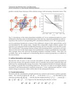
The trajectory and contour error appearing in the multi-axis machine tools are
shown in Fig. 5.3. P is the current position, and R denotes the reference point to go
to. The purpose of tracking control is to minimize the position errors of each axis, e
x
,
e
y
, which are the deviation of the current position from the reference point. On the
other hand, contour control is implemented to minimize the contour error,
ε
,which
is the error of the current position to the desired contour. Therefore, the position error
and contour error are used as the indices for evaluating the accuracy of the controlled

path.
The position error is the linear distance between the actual tool position and the
reference point, and is represented like Eq. 5.1 by using the position error of each
axis.
e =

(e
x
)
2
+(e
y
)
2
(5.1)
where, e denotes the position error and e
x
and e
y
denote the position error of X-axis
and Y-axis respectively. The contour error,
ε
, is the minimum distance between the
actual tool position and the desired path, as shown in Fig. 5.3.
Minimising the position error of each axis does not always mean the reduction of
the contour error. In the case of cutting machine tools, the accuracy of the final ma-
chined shape is the important factor, therefore reduction of the contour error should
be considered more seriously than reduction of the position error.
In general, point-to-point control is used for controlling the movement to the com-
manded position within a short settling time, regardless of the intermediate path, by

utilizing a P controller or PI controller. Compared with point-to-point control, how-
5.4 Position Control 161
X-axis
Y-axis
Reference point
R
e
y
ex
P
Actual path
E
Desired path
Tool
E: Contour error R: Reference position
e
x, ey : Axial errors P: Actual position
Fig. 5.3 Difference errors between real and reference points
ever, tracking control and contour control have many problems to be considered. Be-
cause of inherent system specific errors, including disturbance, friction force, back-
lash, distortion of table, and the characteristics of the servo system as well as dynamic
errors due to high speed operation of the servo system, acceleration or deceleration
operation, and the change of movement direction, some difference between the de-
sired path and the actual controlled path cannot be avoided during contour machining
by multi-axis machine tools.
Therefore, in the position controller of a CNC system there is a variety of control
algorithms, including the P controller, PID controller, fuzzy controller, feed-forward
controller, predictive controller, and cross-coupling controller that have been intro-
duced to support point-to-point control, tracking control, and contour control.
Compared with the P controller, feedback controllers such as the PID controller

and the Fuzzy controller decrease the position errors of each axis. The feed forward
controller is useful for reducing the multi-axis error by reducing the axial error of
each axis, and finally contributes to reduction of the contour error. The cross coupling
controller performs accurate control in real time by generating control commands to
reduce contour error based on a contour error model. In this textbook, the causes of
various errors and algorithms for reducing the position error will be addressed.
5.4 Position Control
The last task of NCK is the position control task where the reference position from
the interpolator and the actual position fed back from a servo motor (encoder) are
162 5 PID Control System
compared and control to decrease the difference between these two positions is car-
ried out.
A PID controller and a feedforward controller are typical algorithms for carrying
out the position control task and they will be described in the following sections.
5.4.1 PID Controller
Although various modern control theories have been developed, the PID controller
has been widely used in industry due to its simple architecture and ease of imple-
mentation in hardware or software. Furthermore, the PID controller can easily be
implemented, even when an accurate mathematical model of target system is un-
known, and realizes excellent control performances, including target-value following
or disturbance rejection.
However, the PID controller can only be used for time-invariant linear systems
and it is necessary to tune gains accurately based on the dynamics of the process.
When the process dynamics are changed due to change of the system weights, the
gain tuning process should be redone. In addition, the PID controller has the lim-
itation that it can be applied only for SISO (Single Input Single Output) systems.
Because CNC systems generally control more than two axes, they can be regarded
as systems with more than one input and output. However, it is possible to use an
individual PID controller for each axis because each axis of machine tools is actually
independently controlled based on the interpolated data of every tiny interpolation

time interval. Accordingly, each axis is controlled by a PID controller having a single
input and output port.
The PID controller can be utilized as a P controller for only proportional (P)
control actions, an I controller for only integral (I) control actions, and a D controller
for only derivative (D) control actions. It can also be used as a combination of single
controllers such as a PI controller, PD controller as well as PID controller. Actually,
for position control of machine tool axes, a P controller or a PI controller having a
small integral gain has been widely used.
G
c
(s)=K
p
+
K
i
s
+ K
d
s (5.2)
As shown in Fig. 5.4, a PID controller generates the output u as an input of the
process, which makes the error (difference between the process output feedback and
a reference input) zero. The transfer function of the PID controller including the
proportional control action, integral control action, and derivative control action is
represented by Eq. 5.2. Therefore, the design of a PID controller involves the deter-
mination of the proportional gain K
p
, the integral gain K
i
, and derivative gain K
d

.
The proportional control action plays the role of handling the immediate error.
Through the proportional control action, it is possible to decrease the rise time of a
5.4 Position Control 163
system and the steady-state error.However this causes overshoot increase and steady-
state error.
The derivative control action has the role of handling errors based on learning
from the past. With the derivative control action it is possible to decrease overshoot
and settling time. The integral control action has the role of handling future errors.
Using the integral control action, it is possible to remove a steady-state error and
decrease the rise time of a system. However, this causes an increase of overshoot and
settling time.
PID Controller
Process
r
+
e
u
y
Fig. 5.4 Block diagram of position control in PID
G
c
(s)=K
p
(1 +
1
T
i
s
+ T

d
s) (5.3)
The transfer function in Eq. 5.2 can be rewritten as Eq. 5.3 where the integral time
T
i
and derivative time T
d
are defined as in Eq. 5.4a and Eq. 5.4b, respectively.
T
i
= K
p
/K
i
(5.4a)
T
d
= K
d
/K
p
(5.4b)
The following gives more details about control actions of each component in a
PID controller. First, in P control, meaning proportional control, the system error
is multiplied by a constant P, called the proportional gain, in order to compensate
for the system error. Therefore, larger proportional gain typically results in faster
response of a system and decreases the time spent in going to the reference point.
However, because large proportional gain makes it impossible to regulate accurately
the system error, there is continuous vibration and abnormal noise. Therefore, the
amount of the proportional gain is restricted due to this reason.

Second, I control, meaning integral control, is used in the case of not going to
the reference point after transition to the steady state. In I control, the error is in-
tegrated over a period of time, multiplied by a constant I, called the integral gain,
to reduce the integrated errors from the past. Larger integral gain results in faster
response during transition states. Accordingly, it is necessary to use an integral gain
within an adequate range because large integral gain results in excessive overshoot
or undershoot.
Third, in D control, meaning derivative control,thefirst derivative over time (the
slope of the error) is calculated, and this derivative is multiplied by a constant D,
called the derivative gain, for damping the system and removing the vibration of
a system during a steady state. Larger derivative gain results in a faster response.
However, large derivative gain causes vibration of a system. Therefore, the amount
164 5 PID Control System
of the derivative gain should be restricted because the first derivative of position over
time is sensitive to noise.
Above, the effect of different types of gain on the PID controller is explained.
Therefore, in practice, a variety of combinations of P control, I control, and D control
has been selectively used according to the purpose for which the control is used.
Typically, the PI controller which has a relatively fast response has been widely used
because D control has difficulty in gain tuning and easily results in vibration.
The transfer functions for the proportional controller, the integral controller,
and the derivative controller defined in a continuous time domain can be approxi-
mated by the transfer functions for the discrete time domain for digital control as in
Eqs. 5.5, 5.6 and 5.7.
G(s)=K
p
⇔ G(z)=K
p
(5.5)
G(s)=

K
i
s
⇔ G(z)=
K
i
T
1 −z
−1
(5.6)
G(s)=K
d
s ⇔ G(z)=
K
d
(1 −z
−1
)
T
(5.7)
By combining the above three approximated equations, the transfer function for
the PID controller for discrete time domains can be approximated as in Eq. 5.8.
G
c
(z)=
k
0
+ k
1
z

−1
+ k
2
z
−2
1 −z
−1
(5.8)
where, k
0
= k
p
+ k
i
T +
k
d
T
, k
1
= −k
p
−
2k
d
T
,andk
2
=
k

d
T
and T denotes the iteration
time for position control. Accordingly, the output of the digital PID controller with
proportional, integral, and derivative control can be represented as the difference
equation, as in Eq. 5.9.
u
e
=
k
0
+ k
1
z
−1
+ k
2
z
−2
1 −z
−1
(5.9a)
or, u(n) −u(n−1)=k
0
e(n)+k
1
e(n −1)+k
2
e(n −2) (5.9b)
Equation 5.9b can be rewritten as Eq. 5.10.

u(n)=u(n −1)+k
0
e(n)+k
1
e(n −1)+k
2
e(n −2) (5.10)
Consequently, in the PID controller for the discrete time domain, the input of
the controller at the current time is computed based on the controller’s input at the
previous iteration time, the error at the current time, the error at the previous iteration
time (one step behind the current sampling time), and the error at the time before that
(two steps before the current sampling time).
For example, when the PID controller is used for controlling a rotary table, the
block diagram for position control of the complete system is as shown in Fig. 5.5.
5.4 Position Control 165
Assume that the transition function for the particular axis of a rotary table is defined
as in Eq. 5.11.
Gc(z)
command
err
u
pos
Gm(z)
Fig. 5.5 Block diagram for controlling rotary table system
Gm(z)=
a
1
z
−1
+ a

2
z
−2
+ a
3
z
−3
1 + b
1
z
−1
+ b
2
z
−2
+ b
3
z
−3
(5.11)
When Eq. 5.11 is expressed as the relationship between the controller output sig-
nal u and the actual position, pos, the discrete form with respect to the current itera-
tion time, k, can be denoted as in Eq. 5.13.
pos(k)=b1 ∗pos(k −1)+b2∗pos(k −2)+b3∗pos(k −3)+ (5.12)
a1 ∗u(k−1)+a2 ∗u(k−2)+a3 ∗u(k −3)
The actual position data detected from the servo is fed back as the input to the PID
controller. The actual position data is compared with the command position data from
the interpolator and the position error between the actual position and the command
position data is input to the PID controller. Finally, the PID controller generates the
output signal u for reducing the error, and signal u is fed to the controlled system

Gm(z).
According to the above example, the program for realizing the PID controller for
position control can be written as follows:
Procedure PID
Controller()
{
/ Setting process variables /
a1=0.007001; a2=0.017284; a3=0.002475;
b1=1.782; b2=-0.906; b3=0.124; /Process parameters/
tpos=0.001; / PID gain setting /
zkp=2.0; zki=0.0001; zkd=0.0;
/Here, only PI schema is applied, I gain needs to be very low./
zk0=zkp+zki*tpos+zkd/tpos;
zk1=-zkp-2*zkd/tpos;
zk2=zkd/tpos;
/ Initialisation of control variables /
err1=0.0; err2=0.0; command=0.0; feedback=0.0;
166 5 PID Control System
pos=0.0; pos1=0.0; pos2=0.0; pos3=0.0;
u=0.0 u1=0.0; u2=0.0; u3=0.0;
err=0.0; err1=0.0; err2=0.0;
begin (n=1,200)
pos
command(n)=10.0-real(n)*0.02; /Generation of position/
/command for simulation/
pos
command (n+100)=8.0+real(n)*0.02;
end / Position control loop /
begin (n=1, 300)
command= pos

command (n); /Command value for position control/
feedback=pos ; /Position feedback/
err=command - feedback; /Error/
u=u1+zk0*err+zk1*err1+zk2*err2; /PID control algorithm, Eq. 5.10/
/Transfer equation for rotary table, Gm, Real position simulation/
/by Eq. 5.10/
pos=b1*pos1+b2*pos2+b3*pos3+a1*u1+a2*u2+a3*u3;
/Update for the next position loop/
pos3=pos2; pos2=pos1; pos1=pos;
u3=u2; u2=u1; u1=u;
err2=err1; err1=err;
end
}
As shown above, it is easy to implement the PID controller for motion control.
However, the performance of the PID controller depends highly on the P, I, and D
gain according to the given environment. Whenever an operating point or the charac-
teristic of the target process changes, it is necessary to tune the gains. The way to set
the P, I, D gain is called the “gain tuning method” and an expert is typically required
for gain tuning.
In the next section, a gain tuning method for the PID controller will be introduced.
5.4.2 PID Gain Tuning
If adequate gain for the PID controller is not set, the system response may become
slow, vibration may occur, or the desired accuracy may not be achieved. Therefore,
setting adequate gains is an important design factor.
As the gain tuning method for a PID controller, there are the Ziegler–Nichols
method, where a mathematical model for the target process are not necessary, and
the Relay method. For these methods, a user with a lot of experience should tune P, I,
D gain by trial and error and, therefore, it takes a long time to complete gain tuning.
As gain tuning methods based on a target process model, there are the Frequency
response method, the Pole placement method, and the Pole-zero cancelation method.

However, because of the complication of the mathematical model for the target pro-
5.4 Position Control 167
cess, it is difficult to derive the model of a target process in practice. Furthermore,
because the experiment for obtaining frequency response is complicated and it is dif-
ficult to obtain an accurate result, the accuracy of the gains tends to decline in the
case when the degree of a system is high. Also, because of the disturbance due to
the load, the pole and zero in the system are not exactly canceled and thereby, the
performance of the system declines.
Recently a controller with an auto tuning function has been developed that tunes
the gains automatically to help users. The auto-tuning function in this controller per-
forms internally advanced gain tuning methods including those mentioned above.
5.4.2.1 The Ziegler–Nichols Method
The Ziegler–Nichols method, which is one of the experiment-based gain tuning
methods, is a method where the target process is tested as an open loop plant and
the P, I, and D gains related to the characteristic of the transient response are cal-
culated by simple formatted equations. This gain tuning method can be executed in
two ways; the first is the step response method based on the response curve of the
process and the second is the ultimate sensitivity method.
The step response method is a gain tuning method using the damping ratio of 0.25
from experiment and experience where the dominant transition diminution becomes
25% of the previous one after one cycle in the time domain. This method can be
applied to a safe system where oscillation does not occur because the main polar-
pole of the target process is not a complex conjugate, and typically a system having
an S-shaped response curve satisfies this condition.
After the step pulse is applied to the system, the S-shape response curve is
achieved. By analyzing the S-shape response curve, various characteristic param-
eters (response delay time, time constant) can be extracted, and, finally, the gains for
the PID controller are calculated by the equations shown in Table 5.1.
The ultimate sensitivity method is useful for a target process that has poles at the
origin or unstable poles resulting in system oscillation. For the the ultimate sensi-

tivity method, first set T
i
= ∞, T
d
= 0 in Eq. 5.3, and increase the proportional gain
step by step. When system oscillation is detected, a critical gain (K
u
) and critical
frequency (T
u
) can be extracted. Finally, the PID controller’s gains are obtained by
the equations shown in Table 5.1. If system oscillation does not occur, even when the
proportional gain is increased, this method cannot be applied.
The Ziegler–Nichols method is good and simple for gain tuning, but needs a fine
tuning process by a tuning expert. Also, it cannot achieve satisfactory control perfor-
mance in the case of a system having small damping characteristics.
As an automatic gain tuning method for a PID controller, a relay method is com-
bined with the Ziegler–Nichols frequencyresponse method to extract the critical gain
and critical frequency. Besides these, various techniques, including adaptive control
theory, optimization theory, and fuzzy control theory have previously been devel-
oped. Please refer to the bibliography for details of each technique. In this book, the
168 5 PID Control System
Table 5.1 Ziegler–Nichols Method
Control Step Response Ultimate Sensitivity Method
Condition Step response has S-shape As proportional gain
increases, output oscillates
Procedure 1. By inputting step pulse 1. By setting T
i
= ∞ and
to target, generate T

d
= 0 in closed loop system,
S-shaped response. activate only proportional
2. Draw tangent line on control loop.
point of inflection of 2. Until output c(t) keeps
output. From intersection oscillating, regulate K
p
points where tangent line 3. Proportional gain at
meets time axis and moment of oscillation is kept
response K, calculate to critical gain K
u
.Set
response delay time
τ
d
critical frequency T
u
to
and time constant
τ
frequency at this moment.
Output
response
t
C(t)
k
τ
d
τ
T

u
t
C(t)
Ctrl. P K
p
=
τ
/
τ
d
K
p
= 0.5K
u
eqn. PI K
p
= 0.9
τ
/
τ
d
,T
i
= 3.3
τ
d
K
p
= 0.45K
u

,T
i
= 0.8T
u
PID K
p
= 1.2
τ
/
τ
d
,T
i
= 2
τ
d
, K
p
= 0.6K
u
,T
i
= 0.5T
u
T
d
= 0.5
τ
d
T

d
= 0.125T
u
relay method that is commercially applied in the industrial field, will be explained in
detail.
5.4.2.2 Relay Gain Tuning
The Ziegler–Nichols method mentioned above has the limitation that it cannot be
applied to a system that is not critically oscillated with only proportional gain con-
trol. To overcome the non-oscillating problem, a relay gain tuning method was in-
troduced. In this method, a relay is utilized for system oscillation by force. When
oscillation occurs, the limits of frequency and amplitude are extracted from the sys-
tem response.
The circuit for the relay-based automatic gain tuning method consists of the con-
ventional PID controller, a relay, and a switch for switching reference input. The
relay and the switch are located in front of the PID controller, as shown in Fig. 5.6.
The difference between the reference input, r, and the process output, y, is input to
the relay. The output of the relay is directly input to the PID controller. At the initial
5.4 Position Control 169
stage of gain tuning, the switch is connected to contact a, thereby the reference input
bypasses the relay and is directly input to the PID controller. Therefore, a non-tuned
PID controller is operated.
At the next automatic tuning stage, the switch is connected to the contact b,and
the difference between the reference input and the process output is fed to the relay.
System oscillation due to the limit cycle phenomena is induced, and the ultimate
frequency and amplitude are extracted for automatic tuning of the PID gains.
PID Controller Process
r
a
b
+

+
e
u
y
.
.
Fig. 5.6 Circuit for relay-based automatic gain tuning
The automatic gain tuning stage can be done as shown in Fig. 5.7a. The relay is
modeled as a system with gain K
R
.Furthermore,G
C
(s) and G
P
(s) mean the transfer
transition function of the PID controller and the process, respectively. The error can
be expressed as Eq. 5.13.
e = K
R
r −y−K
R
y = K
R
r −(1 + K
R
)y (5.13)
If Fig. 5.7a is arranged as the form of the rightmost equation of Eq. 5.13, it can
be denoted as Fig. 5.7b, and the loop transfer function is (1+K
R
)G

C
(s)G
P
(s).
+
+
e
y
.
.
r
K
R
Gc
(s)
G
p
(s)
(a)
+
e
y
.
r
K
R
Gc
(s)
G
p

(s)
(b)
1+KR
Fig. 5.7 Block diagrams of gain setting
While the gain of a relay is expressed using the describing function of non-linear
system theory as Eq. 5.14.
170 5 PID Control System
K
R
=
4d
π
a
(5.14)
where, a is the amplitude of the process output and d denotes the amplitude of the
relay.
At this stage, the process transfer function is assumed to be as in Eq. 5.15 which
is used in the Ziegler–Nichols method and briefly represents the characteristics of
the process.
G
p
(s)=
e
−
τ
s
T
p
s
(5.15)

where, T
p
is the time constant and
τ
stands for the dead time.
On the other hand, the transition function of the PID controller can be represented
as in Eq. 5.16.
G
C
(s)=K
C

1 +
1
T
i
s

T
d
s+1
α
T
d
s+1

(5.16)
where, T
i
and T

d
, respectively, denote the integration time and derivative time and
α
stands for derivative gain.
If oscillation is continuously induced at the moment that the relay is connected
with the PID controller and the automatic gain tuning stage begins, the frequency
and amplitude of the induced oscillation are derived as in the following equations,
arg[(1+ K
R
)G
P
( j
ω
0
)G
C
( j
ω
0
)] = (5.17)
arg

(1 + K
R
)
e
−
τ
s
T

p
s

K
C
(T
i
s+1
T
i
s

T
d
s+1
α
T
d
s+1

s= j
ω
0
= −
π
|(1 + K
R
)G
P
( j

ω
0
)G
C
( j
ω
0
)| = (5.18)




(1 + K
R
)
e
−
τ
s
T
p
s

K
C
(T
i
s+1
T
i

s

T
d
s+1
α
T
d
s+1





s= j
ω
0
= 1
where
ω
0
is the oscillation frequency. The dead time
τ
and time constant T
p
which
show the characteristic of the process can be found using Eqs. 5.19 and 5.20.
τ
=
tan

−1
(T
i
ω
0
)+tan
−1
(T
d
ω
0
) −tan
−1
(
α
T
d
ω
0
)
ω
0
(5.19)
T
p
=
(1 + K
R
)K
C


T
2
i
ω
2
0
+ 1

T
2
d
ω
2
0
+ 1
T
i
ω
2
0

α
2
T
2
d
ω
2
0

+ 1
(5.20)
5.4 Position Control 171
In order to compute PID gains by the estimation of the dead time and time con-
stant from Eqs. 5.19 and 5.20, an ultimate gain and frequency are necessary to use
the equation of the response curve of the Ziegler–Nichols method mentioned in Ta-
ble 5.1. In the case that the Ziegler–Nichols gain tuning method is used, the rela-
tionships between those parameters, the frequency and the amplitude are given by
Eqs. 5.21 and 5.22.
arg[G
P
( j
ω
u
)G
C
( j
ω
u
)] = arg

K
u
e
−
τ
s
T
P
s


s= j
ω
u
= −
π
(5.21)
|G
P
( j
ω
u
)G
C
( j
ω
u
)| =




K
u
e
−
τ
s
T
P

s




s= j
ω
u
= 1 (5.22)
where,
ω
u
denotes an ultimate frequency. From T
u
= 2
π
/
ω
u
, the ultimate frequency
can be obtained from Eq. 5.23.
T
u
= 4
τ
(5.23)
Also, the ultimate gain is given by Eq. 5.24.
K
u
=

2
π
T
P
T
u
(5.24)
Finally, by applying Eq. 5.23 and Eq. 5.24 to the ultimate sensitivity method,
adequate PID gains can be obtained.
The automatic gain tuning method mentioned above is summarized in Fig. 5.8. It
is assumed that the gains of the PID control loop are roughly tuned manually before
executing automatic gain tuning, as depicted in the first and second steps of Fig. 5.8.
In the third step, the relay is connected at the set point input of the PID control
loop. The fourth step means that the process output induces continuous oscillation as
the response of the system when the relay is applied.
In the fifth step, the frequency and the amplitude of the induced oscillation are
measured and stored. In the sixth step, based on measured parameters, the dead time
and the time constant are computed using Eq. 5.19 and Eq. 5.20.
By substituting the dead time and the time constant for Eq. 5.23 and Eq. 5.24,
the ultimate gain and amplitude are computed. Thereby, finally, the PID gains are
computed by the equations of Ziegler–Nichols’s ultimate sensitivity method.
In the seventh step, by decoupling the relay, the set point is coupled to the input
of the PID control loop. In the eighth step, the new PID gains obtained from the sixth
step are applied to the PID control loop.
5.4.3 Feedforward Control
The feedback controller, which is widely used as a servo controller, works based
on the difference between input and output. The PID controller, being one type of
172 5 PID Control System
Crudely tune the PID control loop by any suitable method
PID control loop is running

Apply a relay at the set point input of PID loop
PID control develops a sustained oscillation with the relay
Measure period and amplitude of the sustained oscillation
Calculate new PID parameters based on the measured values
Decouple the relay and couple the set point to the input of PID
Apply the new PID parameters to the PID controller
Fig. 5.8 Automatic gain tuning method
feedback controller, mentioned in the previous section, is very stable and robust even
when there is disturbance. However, tracking error cannot be avoided when only a
PID controller is used. This problem results in a poor cutting surface or inaccurate
shape of the machined product of the CNC machine tool.
As an alternative, a feedforward controller is used together with a feedback con-
troller in order to make up for the feedback controller’s disadvantage and enable a
system to track the desired reference path. The feed-forward controller does not work
based on the difference between the commanded point and the actual point, as does
the feedback controller, but works based on a pre-specified system model. As the
feedforward controller is an open-loop type, it generates the output with calculations
based on the pre-specified system model in order to increase the response charac-
teristics of the complete system. Because of the error in the system model, perfect
control of the complete system cannot be achieved. Therefore, it is typical to use
feedback control and the feedforward control together.
The purpose of the feedforward control method is to overcome the response limi-
tations of a position control loop and feedforward control belongs to tracking control
5.4 Position Control 173
that enables the system to track the desired path by minimizing the tracking error. As
shown in Fig. 5.9, the feedforward controller directly feeds the controller output to
the inner loop by skipping the outer loop, which uses the fact that the response of the
inner loop is faster than the outer loop in a cascade loop structure. Consequently, the
feedforward scheme improves the response characteristics of the outer loop.
Feedforward

Controller
Xw
Controller
Inner Loop
X
M
+
-+
+
Fig. 5.9 Feedforward control placement
The feedforward control method can be classified into two types from the point
of view of the loop structure.
1. After modifying the reference input, the modified input is fed to the feedback
control loop, as shown in Fig. 5.10a.
2. The reference input is directly fed forward to the drive unit in the feedback control
loop, as shown in Fig. 5.10b.
In the first type, G
−1
0
(z), the inverse of the transfer function of the complete sys-
tem including the feedback loop, G(z), is set as the transfer function of the feedfor-
ward control loop. Since the total transfer function of the complete system is set as
G
−1
0
(z)G(z)=1, the actual controlled position and the desired position can become
equal. In the second type, the transfer function of the feedforward controller is set
to be the inverse of the transfer function of the drive unit, D
−1
0

(z). Therefore, the
transfer function of the entire control loop is written as Eq. 5.25.
G
C
(z)=
D
−1
0
(z)D(z)+H(z)D(z)
1 + H(z)D(z)
(5.25)
Consequently, if D
−1
0
(z)D(z)=1 is satisfied, the actual position and the desired
position have come to be the same. In the first type, the inverse transfer function
is very complex because the transfer functions of the feedback controller and the
drive module are included in the inverse transfer function. However, when the inverse
transfer function (G
−1
0
or D
−1
0
) has unstable poles, modification of the feedback con-
troller is necessary. For modification of the feedback controller, the first type is more
suitable than the second.
As typical techniques of the firsttype,ZPETC,IKF,causalFIRfilter, and non-
causal FIR filter will be described in the following subsections.
174 5 PID Control System

+PR
G
0
H(z)
(a)
1
(z)
D(z)
EU
G(z)
H(z) = Controller
D(z) = Drive unit
Feedforward
controller
+
R
D
0
H(z)
1
(z)
E
U
Feedforward
controller
(b)
+
+
D(z)
P

Fig. 5.10 Feedforward control structure
5.4.3.1 ZPETC, Zero Phase Error Tracking Control
Generally, the design of the feedforward controller is based on the transfer function
of the entire system after designing the feedback controller. In considering Fig. 5.10a,
‘R’ denotes the desired path from the interpolator and ‘E’ denotes the error, the
difference between the modified input from the feedforward controller and the output
of process.
The purpose of the feedforward controller is to make P(k) and R(k) equal, or to
minimize the difference between them if it is impossible to make P(k)=R(k).
If the feedforward controller is designed as the inverse of G(z) when G(z) is a
minimum-phase system where poles and zeroes are stable, the transfer function de-
noting the relationship between the input and the output results in 1, which means
that the system traces the desired position correctly. However, the system is not al-
ways a minimum-phase system and some systems can have unstable zeroes. Further-
more, unstable zeroes can be produced when a continuoustime system is transformed
into a discrete time system, even if the system in the continuous time domain has no
unstable zeroes.
The unstable zeroes are located in the left half of the Z-plane of the discrete time
domain. In the case of a non-minimum phase system, if the feedforward controller
is designed as the inverse of G(z), it makes the system unstable because the feed-
forward controller itself can have an unstable pole and the output of the feedforward
controller is unlimited. Therefore, for a non-minimum phase system, it is necessary
to make the transfer function of the entire system close to 1 without making the sys-
tem unstable. Since G(z) is the transfer function including the feedback controller
5.4 Position Control 175
and is designed to make the system stable, the poles of G(z) are stable, in general.
However the transfer function can include unstable zeros because the zero of G(z) is
not restricted. The unstable poles play a role in the poor performance of the system.
Therefore, the feedforward controller is an effective way of removing the unstable
zeroes. The typical algorithm for this is ZPETC (Zero Phase Error Tracking Control).

In ZPETC, the numerator term of the transfer function of a closed loop can be
divided into terms including only the stable zeroes B
s
c
(z
−1
) and terms including only
the unstable zeroes B
u
c
(z
−1
), as shown in Eq. 5.26.
B
c
(z
−1
)=B
s
c
(z
−1
)B
u
c
(z
−1
) (5.26)
Now, the ZPETC feedforward controller can be represented as follows by utilizing
the special numerator term.

G
−1
(z)=
z
d
A(z
−1
)B
u
c
(z)
B
s
c
(z
−1
)(B
u
c
(1))
2
(5.27)
In consequence, the entire transfer function can be summarized as follows,
G
zpetc
(z)=
B
u
c
(z)B

u
c
(z
−1
)
(B
u
c
(1))
2
(5.28)
We can understand that the phase difference of the transfer function from the de-
sired path to output is zero because the transfer function results in the multiplication
of two conjugating complex numbers. This means that the output traces the input
with no time delay, the gain in the steady state is one and the error in the steady state
becomes zero. When the transfer function of a closed loop has an the zeroes located
on the left half of the plane, the gain increases. This means that ZPETC can have the
gain error in the high-frequency range instead of making the phase difference zero.
On the other hand, ZPETC is a good algorithm for building good characteristic by
using small information in the low frequency range. The ZPETC requires an accu-
rate system model, which is somewhat difficult, and shows poor tracing performance
when the desired trajectory includes a fast transient shape such as at sharp corners.
Furthermore, the inverse transfer function of the feedforward controller may require
D/A converters or driving motors capable of handling high voltage, which is practi-
cally limited by the maximum output of D/A converter or the maximum voltage of
the motor.
5.4.3.2 IKF, Inverse Compensation Filter
The IKF(Inverse Compensation Filter) was introduced by Weck to solve the corner-
tracing problem of ZPETC. As shown in Fig. 5.11, a low-pass filter is added at the
front of the feedforward controller to improve traceability. Consequently the smooth

trace becomes possible by removing the high-frequency range from the input signal.
176 5 PID Control System
A(z )
Low-pass
filter
Inverse
system
Position
control loop
IK
R
R*
P
A(z )B (z)
____________
B (z )[B (1)]
+
2
z B (z )B (z )
_______________
d
+
1
1
1
1
1
Fig. 5.11 IKF filter structure
5.4.3.3 Causal/Non-causal FIR
The controllers mentioned in the previous sections require an accurate system model

and the transfer function is formulated using a complicated process. However, it is
difficult to apply these controllers to a real CNC system. Therefore, a practical tech-
nique is typically used in industry, where the position command is forwarded to the
feedback controller together with velocity and acceleration/deceleration commands,
as shown in Fig. 5.12.
_____
_____
w (k)
1
1 z
1
T
T
w (k)
1
w (k)
2
w (k)
3
V *
2
V *
3
K
y
K
p
u(k)
process
x (k)

x (k)
1
2
(a)
w (k)
1
K
y
K
p
u(k)
process
x (k)
x (k)
1
2
(b)
a + a z +a z
2
1
1
0
2
1 z
1
Fig. 5.12 Practical feedforward control
This type of controller can be represented mathematically in the two-step causal
filter as Eq. 5.29.
5.4 Position Control 177
G(z)=a

0
z
−2
+ a
1
z
−1
+ a
2
(5.29)
where, a
0
=
V
3
T
2
, a
1
= −
V
2
T
−
2V
3
T
2
, a
2

= 1+
V
2
T
+
V
3
T
2
The above causal FIR filter uses the current position data and the position data
from one and two steps before. It can also be represented in the non-causal FIR filter
form that requests future position data.
G(z)=a
0
+ a
1
z+a
2
z
2
(5.30)
The architecture of the controller can be as shown in Fig. 5.13.
w (k)
1
K
y
K
p
u(k)
process

x (k)
x (k)
1
2
a + a z +a z
0
12
2
Fig. 5.13 Non-causal FIR
In a modern CNC system, the above non-causality, asking the future status value
of CNC, can no longer be an obstacle. Since the CNC system typically stores
the future position by NC block interpretation and position interpolation (e.g. lin-
ear/circular interpolation), the future position information at the current position can
be obtained by reading the memory location. The time delay due to the degree of the
filter and position sampling time may occur between the moment that an interpreter
completes interpreting the NC block and the moment that actuation begins. However,
this does not have any effect on the control performance and, actually, this control
type is not worse than the other feedforward controller with respect to the contouring
accuracy and the traceability at corners.
In the previous sections as well as in the current section, the feedforward con-
troller that modifies the input signal and feeds the modified input to the feedback
controller has been described. The following sections describe a controller where the
input signal is fed directly to the feedback controller. A speed feedforward controller
and a torque feedforward controller are typical of this kind of controller. This type
of feedforward controller requires advanced control theories such as speed control
and torque control of the servo system. In this book, only the basic architecture will
be introduced. For other details, please read the reference on design of digital drive
systems.
Figure 5.14 shows the architecture of a speed feedforward controller where the posi-
tion command,

α
w
,isfiltered and the filtered command is input directly to the speed
control loop in a drive system in order to improve the response of the position control
loop. K
v
in Fig. 5.14 denotes the proportional gain of the position controller and only
5.4.3.4 Speed Feedforward Controller
178 5 PID Control System
proportional control is used for the position control of a CNC system. K
pn
and K
in
in Fig. 5.14 denote a propositional gain and an integral gain of the speed controller,
respectively, and it is typical that a PI control is used for the speed control of a CNC
system.
α
w
and
α
denote the desired position and the actual position respectively,
and T is the sampling time of the position control loop.
Hα
System
to be controlled
H
n
Kv
Position
Controller

Kin
z
z 1
___
K
pn
T
Simple
&
Holder
Speed Control Loop
Position Control Loop
Speed Control
Feedforward
Controller
α
α
w
Fig. 5.14 Architecture of speed feedforward controller
Figure 5.15 shows the architecture of a torque feedforward controller. In the torque
feedforward controller, a position command is directly input to the current loop (e.g.
system to be controlled) that shows the fastest system response. Therefore, in the
torque feedforward controller, the speed control loop including a current loop inside
ward controller generates the position command that is directly input to the current
loop, the speed command from an interpolator is used as an input to the feedforward
controller for stable control. Because the torque feedforward controller actuates the
motors by using the current loop with the fastest response, it generates the minimum
following error under serial control architecture.
By using the feedforward controller for machine tools, the following error of the
position control loop drastically decreases. The following error will be described in

detail in the next section.
5.4.3.5 Torque Feedforward Controller
and position control loop should fulfill the input balance. Since the torque feedfor-
5.5 Analysis of the Following Error 179
Hα
System
to be controlled
H
n
Kv
Position
Controller
Kin
z
z 1
___
K
pn
T
Simple
&
Holder
Speed Control Loop
Position Control Loop
Speed Control
Feedforward
Controller
α
H
m

Fig. 5.15 Architecture of a torque feedforward controller
5.5 Analysis of the Following Error
The following error is defined as the difference between the desired position and
the actual position of the CNC system. Since the position controller is typically a
proportional controller, large proportional gain has an influence on the short setting
time of machine tools. However, it has a limitation due to the steady-state error and
overshoot.
5.5.1 The Following Error of the Feedback Controller
In a typical position control loop, a Unit Feedback System can be represented as in
the block diagram shown in Fig. 5.16.
The transfer function of an open loop, G(s), is generally represented as follows.
G(s)=
K
s
l
·
(1 + sT

1
)(1 + sT

2
) (1 + sT

m
)
(1 + sT
1
)(1 + sT
2

) (1 + sT
n
)
(5.31)
where, l + n ≥ m and K denotes the gain of the controller.
In this case, the position error is defined as the difference between the desired
position and the output position.
E(s)=U(s)−Y(s) (5.32)
180 5 PID Control System
Position
command
Position
error
Open-loop
Transfer function
E(s)
U(s)
Y(s)
Motor
position
G(s)
+
-
Fig. 5.16 Unit feedback controller
The transfer function of a closed loop, W(s), can be written as follows,
W(s)=
Y(s)
U(s)
=
G(s)

1 + G(s)
(5.33)
From Eq. 5.32 and Eq. 5.33, E(s) is summarized as follows,
E(s)+
1
1 + G(s)
U(s) (5.34)
where the steady state error is denoted by e(∞),beinge(t) as t → ∞, and it can be
calculated by using the Final Value Theorem for Laplace transformations,
e(∞)=lim
t→∞
e(t)=lim
s→0
sE(s) (5.35)
If we consider the steady-state error e(∞) when the input is a step input.
The steady state error e
p
for the step input u(t)=A or U(s)=
A
s
is summarized
as follows by using Eqs. 5.31, 5.34, and 5.35.
e
p
= lim
s→0
sE(s)
= lim
s→0
s·

1
1 +
K
s
l
·
(1+sT

1
)(1+sT

2
) (1+sT

m
)
(1+sT
1
)(1+sT
2
) (1+sT
n
)
·
A
s
= lim
s→0
s·
1

1 +
K
s
l
·
A
s
= lim
s→0
A
1 +
K
s
l
(5.36)
Consequently, the steady state error is obtained from Eq. 5.36 as follows,
if l = 0thene
p
=
A
1+K
if l ≥ 1, then e
p
= 0
5.5 Analysis of the Following Error 181
wherein, l = 1 means that G(s) or the controlled system includes the integral element
1
s
. If the number of the integral elements is more than one, e
p

is equal to zero then
the steady-state error does not occur.
Now find the normal error, e(∞), if the input is a Ramp input.
In the case of u(t)=At or U(s)=
A
s
2
, the steady-state error e
p
can be expressed
as follows,
= lim
s→0
s·
1
1 +
K
s
l
·
(1+sT

1
)(1+sT

2
) (1+sT

m
)

(1+sT
1
)(1+sT
2
) (1+sT
n
)
·
A
s
2
= lim
s→0
s·
1
1 +
K
s
l
·
A
s
2
= lim
s→0
A
1 +
K
s
l−1

(5.37)
Finally,
if l = 0thene
p
= ∞.
if l = 1thene
p
=
A
K
.
if l ≥ 2thene
p
= 0.
By utilizing the same method, if the steady state error e
p
due to the acceleration
input u(t)=
A
2
t
2
is considered the result is expressed as:
If l = 0,1, then e
p
= ∞.
If l = 2, then e
p
=
A

K
.
If l ≥ 3, then e
p
= 0.
In this moment, the steady state errors of the feedback controller with respect to
the inputs can be summarized as Table 5.2.
Consequently, if we assume that the input command is a function of time, u(t)=
Vt×t (where,Vt is the commanded feedrate in the CNC system), the following error
is typically as in Eq. 5.38.
e
fbc
=
V
t
K
v
(5.38)
Therefore, we conclude that the following error is inversely proportional to the
gain of the position controller and is proportional to the feedrate when only feedback
control is used. In consequence, it is necessary to increase the gain of the position
controller or decrease the feedrate in order to decrease the following error.
182 5 PID Control System
Table 5.2 Normal error summary
Input u(t)
Desired position Step input
u(t) = A
Desired position
Ramp input
u(t) = at

t
t
Desired position
Acceleration input
u(t) = t
b
__
2
2
ep
=
l = 0:
l >= 1: 0
A
_____
1+k
Desired position
if l = 0
A
_____
1+k
t
Steady state error
Example of steady state error
e
p
=
l = 0:
l >= 2: 0
l = 1:

a
___
K
ep
=
l = 0, 1:
l >= 3: 0
l = 2:
b
___
K
Desired position
if l = 2
b
___
K
if l = 1
Desired position
a
___
K
t
t
t
5.5.2 The Following Error of the Feedforward Controller
If we summarize the following error of the speed feedforward without the compli-
cated derivation process, it can be expressed in short form as Eq. 5.39.
e
v
ffc

= V
t
T
en
(5.39)
The following error of the torque feedforward controller can written as Eq. 5.40.
e
t
ffc
= V
t
(T
ei
+ T/2) (5.40)
where V
t
, T
en
, T
ei
,andT stand for the feedrate, the time constant of the speed control
loop, the time constant of the current loop, and the sampling time, respectively.
Without the feedforward control we already know that the following error in-
creases in proportion to the feedrate and is inversely proportional to the gain of the
position controller, K
v
. Now, when the speed feedforward control is applied, the fol-
5.5 Analysis of the Following Error 183
lowing error is in proportion to the feedrate V
t

and the time constant of the speed
control loop, T
en
.ThismeansthatK
v
, the gain of the position controller does not
have any effect on the following error and plays the role of regulator against external
disturbance when the speed feedforward controller is used. In the case of the torque
feedforward controller, the following error of the system is in proportion to the fee-
drate, time constant of the current loop and the sampling time of the position control
loop.
5.5.3 Comparison of Following Errors
In the previous section, the main factors of the following errors of the feedback
controller, the speed feedforward controller, and the torque feedforward controller
were discussed. These main factors will be simulated by using actual machine tools,
and the result of the simulation will be addressed in this section.
Figure 5.17a shows the commanded position data (the desired position) and actual
position data after simulating without the feedforward controller. As shown in the
figure, the actual position data follows the desired position with a time delay and the
difference between them is called the following error. Figure 5.17b shows only the
amount of the following error and we can investigate whether the following error
converges to the value derived from Eq. 5.38. This following error is multiplied by
K
v
, the gain of the position controller, and the multiplied value is fed to the speed
control loop.
Commanded
position
Actual
position

050
100
150
200
250 300
5
10
15
20
25
30
35
40
45
Time (ms)
Position (mm)
050
100
150
200
250 300
0.5
0.1
1.5
2.0
2.5
3.0
3.5
4.0
4.5

Time (ms)
Following error (mm)
Fig. 5.17 Comparison of following errors
In the case of the speed feedforward controller, it is assumed that the gain of the
position controller and feedrate are equal to the previous simulation, and the time
constant of the speed control loop, T
en
, is assumed to be 4 ms for the simulation.
When the speed feedforward controller is used, the divergence of the following
error can be calculated from Eq. 5.39 as follows,
e
v
ffc
= V
t
T
en
= 0.6667[mm]
184 5 PID Control System
Figure 5.18a shows the following errors when the speed feedforward controller is
used and when the speed feedforward controller is not used. As shown in the figure,
the following error decreases appreciably when the speed feedforward controller is
used. We can also verify that the following error converges to the above calculated
value when speed feedforward control is applied.
In the torque feedforward controller, the command data for actuating the axis is
directly input to the current control loop. Because the current control loop has the
fastest response, theoretically this architecture makes it possible to build a system
with the smallest following error. When the torque feedforward controller is used,
the convergence of the following error can be calculated from Eq. 5.40.
e

t
ffc
= V
t
(T
ei
+ T/2)=0.771[mm]
Figure 5.18b shows the following errors when the speed feedforward controller is
used and when the torque feedforward controller is used. For the simulation, the time
constant of the speed control loop for the speed feedforward controller is specified
as 4 ms and the time constant of the speed control loop for the torque feedforward
controller is specified as 0.4 ms. As shown in the figure, it is possible to decrease the
following error by using the torque feedforward controller.
050
100
150
200
250 300
0.5
0.1
1.5
2.0
2.5
3.0
3.5
4.0
4.5
Time (ms)
Following error (mm)
Speed

Feedforward
No Feedforward
0
50
100
150
200
250 300
0.1
0.2
0.3
0.4
0.5
0.6
0.7
Time (ms)
Following error (mm)
Speed
Feedforward
Torque
Feedforward
Fig. 5.18 Following errors when using speed feedforward
The following error of the position control system is not a critical problem in the
case of a one-axis system. However, in the case of multi-axis systems, the follow-
ing error is reflected in the accuracy of the machined shape. Therefore, it is very
important to decrease the following error for machine accuracy.
As a summary, for the control of a CNC system, the PID controller is a typical
feedback controller for decreasing the position error of each axis. The feedforward
controller is used for decreasing the following error of the PID controller alone.
The feedback controller and the feedforward controller are mutually combined to

decrease the position error of each axis for multi-axis systems.