Rules of Thumb for Mechanical Engineers 2010 Part 2 ppt

Fluids
15
Open-Channel
Flow
Measurements
A
weir
is
an
obstruction in the flow path, causing flow to
back up behind it and then flow over or
through
it (Figure
7).
Height of the upstream fluid is a function
of
the
flow
rate.
Bernoulli’s equation establishes the weir relationship:
the head
of liquid above the weir. Usually,
a
correction co-
efficient is multiplied to account for the velocity head. For
a V-notch weir, the equation may be written as:
8
15
Qkomticd
=
-

J2g
tan
For a 90-degree V-notch weir, this equation may be ap-
H2.’
Q
=
CaL
ds
=
C,LH’.’
where
C,
is
the contraction coefficient
(3.33
in
U.S.
units
and
1.84
in
metric units),
L
is
the width
of
weir, and h is
proximated
to
Q

=
CvH?.5,
where
C,
is
2.5
in U.S. units and
1.38
in metric units.
Figure
7.
Rectangular and
V-notch
weirs.
Viscosity
Measurements
Three
types
of
devices
are
used
in
viscosity measure-
ments: cap-
tube viscometer, Saybolt viscometer, and
1-0-
tating viscometer.
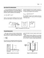
In
a capillary

tube
arrangement (Figure
8),
The reservoir level is maintained constant, and
Q
is deter-
mined by measuring the volume of flow over a specific time
Figure
8.
Capillary tube viscometer.
period. The Saybolt viscometer operates under the same
principle.
In the rotating viscometer (Figure 9), two concentric
cylinders of which one is stationary and the other is rotat-
ing (at constant rpm)
are
used. The torque
transmitted
from
one to the other is measured through spring deflection.
Constant
Temperature
Bath
Figure
9.
Rotating viscometer.
16
Rules
of
Thumb

for
Mechanical Engineers
The shear
stress
z
is
a
function of this torque T. Knowing
shear
stress, the dynamic viscosity may be calculated from
Newton’s law of viscosity.
Td
=
2n~3ho
OTHER
TOPICS
Unsteadv
Flow.
Surre. and Water Hammer
Study of
unsteadyflow
is essential in dealing with hy-
draulic transients that cause noise, fatigue, and wear. It deals
with calculation of pressures and velocities. In closed cir-
cuits, it involves the unsteady linear momentum equation
along with the unsteady continuity
equation.
If
the
nonlinear

friction terms
are
introduced, the system of equations be-
comes too complicated, and
is
solved using iterative, com-
puter-based algorithms.
Surge
is the phenomenon caused by turbulent resistance
in pipe systems
that
gives rise to oscillations.
A
sudden
re-
duction in velocity due to flow constriction (usually due to
valve closure) causes the
pressure
to
rise.
This is
called
water
hammer:
Assuming
the
pipe material to
be
inelastic, the time
taken for the water hammer shock wave from

a
fitting to the
pipe-end and back is determined by: t
=
(2L)/c; the com-
sponding pressure rise is given by: Ap
=
(pcAv)/g,.
In open-channel systems, the surge wave phenomenon
usually results from a gate or obstruction in the flow path.
The problem needs to be solved through iterative solution
of continuity and momentum equations.
Boundary Layer Concepts
For most fluids we know (water or
air)
that have low vis-
cosity, the Reynolds number
pU
Up
is quite high.
So
in-
ertia forces
are
predominant over viscous ones. However,
near
a
wall,
the
viscosity will cause the fluid to slow down,

and have zero velocity at the wall. Thus the study of most
real
fluids can
be
divided
into two regimes:
(1)
near the wall,
a thin viscous layer called the
boundary
layer;
and (2)
outside of it, a nonviscous fluid. This boundary layer may
be laminar or turbulent. For the classic case
of
a flow over
a flat plate,
this
transition takes place when the Reynolds
number reaches a value of about a million. The boundary
layer thickness
6
is given
as
a function of
the
distance
x
from
the leading edge

of
the plate
by:
where
U
and
p
are the fluid velocity and viscosity, respec-
tively.
lift and
Drag
Lifi
and
drag
are
forces experienced
by
a body
moving
through a fluid. Coefficients of lift and drag (CL and C,)
1
2
D
=
-pV2AC,
are
used
to determine the effectiveness
of
the object in

producing these two principal forces:
L
=
-~v*Ac,
where
A
is the reference
area
(usually projection
of
the
ob-
ject’s area either parallel or
normal
to the flow direction),
p
is the density, and V
is
the flow velocity.
1
2
Fluids
17
~~ ~ ~ ~~
Oceanographic
Flows
The pressure change in the ocean depth is dp
=
pgD, the
same

as
in any static fluid. Neglecting salinity, compress-
ibility, and thermal variations, that is about
44.5
psi per
100
feet of depth.
Far
accurate determination, these effects must
be considered because the temperature reduces nonlinear-
ly
with depth, and density increases linearly with salinity.
The
periods
of an ocean wave vary from less than
a
second to about 10 seconds; and the wave propagation
speeds vary from a
ft/sec
to about
50
ft/sec.
If
the wave-
length is
small
compared to the water depth, the wave
speed is independent of water depth and is a function only
of the wavelength:
Tide

is caused by the combined effects of solar and
lunar
gravity. The average interval between successive high wa-
ters
is
about 12 hours and
25
minutes, which is exactly one
half
of the
lunar
period
of
appearance
on the
earth.
The
lunar
tidal forces
are
more
than
twice that of the solar ones. The
spring
tides
are
caused
when
both
are

in
unison,
and the neap
tides
are
caused when they are
90
degrees out of phase.
Heat
Transfer
Chandran
6
.
Santanam. Ph.D.,
Senior Staff Development Engineer. GM Powertrain Group
J
.
Edward Pope. Ph.D.,
Senior Project Engineer. Allison Advanced Development Company
Nicholas P
.
Cheremisinoff. Ph.D.,
Consulting Engineer
Introduction

19
Conduction

19
Single Wall Conduction

19
Composite Wall Conduction

21
The Combined Heat Transfer Coefficient
22
Critical Radius
of
Insulation
22
Convection

23
Dimensionless Numbers

23
Correlations

24
Radiation

26
Emissivity

27
View Factors

27
Radiation Shields

29
Finite Element Analysis

29
Boundary Conditions

29
2D Analysis

30
Evaluating Results 3
1
Typical Convection Coefficient Values

26
Transient Analysis

30
Heat Exchanger Classification

33
Types of Heat Exchangers

33
Shell-and-Tube Exchangers
36
Tube Arrangements and Baffles

38

Shell Configurations

40
Miscellaneous Data

42
Heat Transfer

42
Flow Regimes

42
Flow Maps

46
Estimating Pressure Drop

48
Flow Regimes and Pressure Drop in 'Itvo-Phase
18
Heat Transfer
19
INTRODUCTION
This
chapter will cover the three basic types of heat
transfer: conduction, convection, and radiation. Addition-
al sections will cover finite element analysis, heat ex-
changers, and two-phase heat transfer.
Table
2

Physical Constants Important in Heat Transfer
Constant
Name
Value
Units
Parameters commonly used
in
heat transfer analysis
are
Avagadro's
number
6.0221 69*1
Om
Kmor
ft-lb/lbml"F
Gas
constant
53.3
listed in Table
1
along with their symbols and units. Table
constant
6.6261 96'10-34
J.s
2
lists relevant physical constants.
Bolkmann constant
1.38062Pl
P
JIK

Speed
of
light
in
vacuum
91
372300
Wsec
Stefan-Boltzmann constant
1.71 2"l
P
Btu/hr/sq.W~
latmpressure
14.7
psi
Table
1
Commonly
Used
in Heat Transfer Analysis Parameters
Paramgters
Length
Mass
lime
Current
Temperature
Acceleration
Velocity
Density
Am

Volume
Viscosity
FOW
Kinematic viscosity
Specific
heat
Thermal conductivity
Heat energy
Convection coefficient
Hydraulic diameter
Gravitational
constant
Units
feet
pound
mass
hour or
seconds
ampere
Fahrenheit or Rankine
feeVsecs2
Wsec
poundlcu.
ft
sq.
feet
cubic
feet
IbmlWsq.
see

pound
feetVsec2
Btu/hr/lbPF
Btu. in/ft2/hrPF
Btu
Btu/sq. fVhrPF
feet
Ibm.ft/lbf.sec*
Symbols
L
m
I
T
a
V
P
A
CI
F
CP
k
Q
h
g
z
V
u
Dh
Single
Wall

Conduction
(TI
-
T2)
Area
If
two sides of a flat wall
are
at different temperatures,
k
conduction will occur (Figure
1).
Heat will flow from the
hotter location to the colder point according to the equation:
=
michess
T1
t9t.
For
a
cylindrical system, such as in pipes (Figure
2),
the
equation becomes:
(To
-
Ti
1
Q
=

2n;
(k)
(length)
In (ro/ri)
+X
Figure
I.
Conduction through
a
single
wall.
20
Rules
of
Thumb for Mechanical Engineers
Figure
2.
Conduction through
a
cylinder.
The equation for cylindrical coordinates is slightly dif-
ferent because the area changes as you move radially out-
ward. As Figure 3 shows, the temperature profde
will
be
a straight line for a flat wall. The profile for the pipe will
flatten as
it
moves radially outward. Because area increases
with radius, conduction will increase, which reduces the

thermal gradient.
If
the thickness of the cylinder is small,
relative to the radius, the Cartesian coordinate equation
will give
an
adequate answer. Thermal conductivity is a ma-
terial property, with units of
Btu
FLAT
WALL
CYLINDER
Temp.
X
Radius
Figure
3.
Temperature profile for
flat
wall
and cylinder.
Tables
3
and
4
show conductivities for metals and com-
mon building materials.
Note
that the materials
that

are
good
electrical conductors (silver, capper, and
aluminum),
are
also
good conductors of heat. Increased conduction
will
tend to
equalize temperatures within a component.
Example.
Consider a flat wall with:
Thickness
=
1
foot
Table
3
Thermal Conductivity
of
Various
Materials
at
0°C
Metals:
silver
(pure)
copper
(pure)
Aluminum

(pure)
NiCkel(pure)
0
Carbon
steel,
1
%
C
Lead
(Pure)
Chrome-nickd
SM
(18%
a,
8%
NO
Quartz,polralleltOaxis
wte
Marble
sandstone
Glass,
window
Maple or
oak
sawdust
Glasswool
Liquids:
Mercury
Water
Lubricating

oil,
WE
50
Freon
12,
CQzFs
Hydrogen
Helium
Air
Water
vapor
(saturated)
Carbon
dioxide
Nonmetatlic
solids:
Om:
wwc
410
385
93
73
43
35
16.3
202
41.6
4.15
208-2.94
1.83

0.78
0.17
0.059
0.038
8.21
0.5%
0.540
0.147
0.073
0.175
0.141
0.m
0.0206
0.0146
237
223
117
54
42
25
20.3
9.4
24
2.4
1.21.7
1.06
0.45
0.096
0.034
0.022

4.74
0.327
0.312
0.085
0.042
0.101
0.081
0.0139
0.01 19
0.00844
Source:
Holman
[l].
Reprinted
with
permission
of McGraw-Hill.
Area
=
1
foot2
Q
=
1,000
Btu/hour
For aluminum,
k
=
132,
AT

=
7.58"F
For stainless steel,
k
=
9,
AT
=
1
11.1
OF
Sources
1.
Holman,
J.
P.,
Heat Transfez
New York: McGraw-Hill,
2.
Cheremisinoff,
N.
P.,
Heat Transfer Pocket Handbook
1976.
Houston: Gulf Publishing Co., 1984.
Heat Transfer
21
Table
4
Thermal Conductivities

of
Typical Insulating
and Building Materials
Thermal
(kcavm-hr-
"C)
conductivity
-
Matelial
("0
Asbestos
0
0.13
Glass
wool
0
0.03
300
0.09
cork
in
slabs
0 0.03
50
0.04
Magnesia
50
0.05
slag
wool

0
0.05
200
0.M
Common
brick
25
0.34
pbrcelain
95
0.89
1,100 1.70
CtmCEtL?
0
1.2
Fresh
earth
0
2.0
Glass
15
0.60
Rerpencllcular
fibers
15 0.13
Parallel
fibers
u)
0.30
Burnt

clay
I5
0.80
Car-
600
16.0
Sourn:
Chmmisinoff
p]
Mod
-1:
Composite
Wall
Conduction
For the multiple wall system in Figure
4,
the heat trans-
fer rates are:
Obviously,
Q and Area
are
the same for both walls. The
term
thermal
resistance
is often used:
kl
(T,
-
T~)

Area
Thickness,
41-2
=
k2
(T2
-T3)
Area
Thickness,
42-3
=
Q'-2
I
thickness
k
R,
=
High values
of
thermal resistance indicate a good insula-
tion. For the entire system
of
walls in Figure
4,
the over-
all heat transfer becomes:
The effective thermal resistance
of
the entire system is:
thicknessi

R,
=ZR~
=E
ki
Th
ickness=5'
I
k=.
1
Thickness4
"
k=l
Figure 4.
Conduction through
a
composite
wall.
For
a
cylindrical
system, effective thermal resistance
is:
22
Rules
of
Thumb
for
Mechanical
Engineers
Note that the temperature difference across each wall is

proportional to the thermal effectiveness of each wall.
Also
note that the overall thermal effectiveness is dominated
by the component with the largest thermal effectiveness.
Wall
1
Thickness
=
1.
foot
k
=
1.
Btu/(Hr*Foot*F)
R
=
1.h.
=
1.
Wall
2
Thickness
=
5.
foot
k
=
.1
Btu/(Hr*Foot*F)
R

=
5J.1
=
50.
The overall thermal resistance is
5
1.
Because only
2%
of the total is contributed by wall 1,
its effect could be ignored without a significant
loss
in ac-
curacy.
The Combined Heat Transfer Coefficient
TI
-
T3
An
overall heat transfer coefficient may be used to ac-
count for the combined effects of convection and conduc-
tion. Consider the problem shown in Figure
5.
Convection
=
1
/(
hA)
+
thickness

/(kA)
Overall heat transfer may be calculated by:
1
(1
/
h)
+
(thickness
/
k)
U=
Heat transfer
may
be calculated by:
Q
=
UA
(TI
-
T3)
Although the overall heat transfer coefficient is simpler
to
use,
it does not allow for calculation of
TP.
This
approach
is particularly useful when matching test
data,
because all

uncertainties may be rolled into one coefficient instead
of
adjusting
two
Figure
5.
Combined convection
and
conduction through
a
wall.
Critical Radius
of
Insulation
Consider the pipe in Figure
6.
Here, conduction
occurs
through a layer
of
insulation, then convects to the envi-
ronment. Maximum heat transfer occurs when:
k
route.,
-
-
h
-
This
is

the critical
radius
of
insulation.
If
the outer
radius
is less than
this
critical value, adding insulation will cause
an increase in heat transfer. Although the increased insu-
lation reduces conduction,
it
adds surface area, which
in-
creases convection.
This
is most likely
to
occur when con-
vection
is
low
(high
h), and the insulation is poor (high
k).
Figure
6.
Pipe
wrapped

with insulation.
HeatTransfer
23
While conduction calculations
are
straightforward, con-
vection calculations
are
much
more
difficult.
Numerous
cor-
relation types are available, and good judgment must be ex-
ercised in selection. Most correlations are valid only for a
specific range of Reynolds numbers. Often, different rela-
tionships
are
used for various ranges. The user should note
that these may yield discontinuities in the relationship be-
tween convection coefficient and Reynolds number.
Dimensionless Numbers
Many correlations
are
based on dimensionless numbers,
which are used to establish similitude among cases which
might seem very different. Four dimensionless numbers
are
particularly significant:
Reynolds

Number
The Reynolds number is the
ratio
of flow momentum rate
(i.e.,
inertia force) to viscous force.
The Reynolds number is used
to
determine whether flow
is laminar or turbulent. Below a critical Reynolds number,
flow will be laminar. Above a critical Reynolds number, flow
will be turbulent. Generally, different correlations will be
used
to determine the convection coefficient in the laminar
and turbulent regimes. The convection coefficients
are
usu-
ally significantly higher in the turbulent regime.
Nusselt Number
The Nusselt number characterizes the similarity of heat
transfer at the interface between wall and fluid in different
systems.
It
is basically a ratio of convection to conductance:
hl
N=-
k
Prandtl
Number
The Prandtl number is the ratio of momentum diffusiv-

ity to thermal diffusivity of a fluid:
Pr=-
PCP
k
It is solely dependent upon the fluid properties:
For gases, Pr
=
.7
to
1.0
For water,
Pr
=
1
to
10
For liquid metals,
Pr
=
.001 to
.03
For oils,
Pr
=
50.
to
2000.
In most correlations, the Prandtl number is raised to the
.333
power. Therefore, it is not a good investment to spend

a lot of
time
determjning Prandtl number for a gas. Just using
.85
should be adequate for most analyses.
Grashof
W
umber
The Grashof number is
used
to determine the heat
trans-
fer coefficient under free convection conditions.
It
is basi-
cally a ratio between the buoyancy forces and
viscous
forces.
Heat transfer
reqks
circulation, therefore, the Grashof
number (and heat transfer coefficient)
will
rise as the buoy-
ancy forces increase and the viscous forces decrease.
24
Rules
of
Thumb for Mechanical Engineers
Correlations

Heat transfer correlations are empirical relationships.
They
are
available for a wide range of configurations.
This
book will address only the most common types:
Pipe flow
Average flat plate
Flat plate at a specific location
Free convection
*Tubebank
Cylinder in cross-flow
The last two correlations are particularly important for
heat exchangers.
Plpe
Flow
This correlation
is
used to calculate the convection co-
efficient between a fluid flowing through
a
pipe and the pipe
wall
[l].
For turbulent flow (Re
>
10,000):
h
=
.023KRe.8

x
FY
n
=
.3
if surface is hotter than the fluid
=
.4
if
fluid is hotter than the surface
This correlation
[
11 is valid for 0.6
I
P,
I
160 and
L/D
2
10.
For laminar flow [2]:
N
=
4.36
NxK
h=-
Dh
Average Flat Plate
This correlation is used to calculate
an

average convec-
tion
coefficient for a fluid flowing across a flat plate [3].
PVL
P
Re=-
For turbulent flow (Re
>
50,000):
h
=
.037
me8
x
Pr33/L
For laminar flow:
h
=
.664KRe5
x
Pr33/L
Flat Plate
at
a
Specific location
This
correlation is used to calculate a convection coef-
ficient for a fluid flowing across
a
flat plate at a specified

distance
(X)
from the
start
[3].
Re=-
PVX
P
For
turbulent
flow
(Re
>
50,000):
h
=
.0296KRe.*
x
Pr33/X
For laminar flow:
h
=
.332KRe.5
x
Pr33/X
Static Free Convection
Free convection calculations
are
based on
the

product of
the Grashof and Prandtl numbers. Based on
this
product,
the Nusselt number can be read from Figure
7
(vertical
plates) or Figure
8 (horizontal cylinders) [6].
Tube
Bank
The following correlation is useful for in-line banks of
tubes, such as might occur in a heat exchanger [SI:
It
is valid for Reynolds numbers between
2,000
and
40,000
through tube
banks
more than
10
rows deep. For less than
10
rows, a correction factor must be applied
(.64
for
1
row,
.80

for 2 rows,
.90
for 4 rows) to the convection co-
efficient.
Obtaining
C
and CEXP from the table (see
also
Figure
9,
in-line tube rows):
Heat
Transfer
25
H
=
(CWD)
(Re)CEXP (p1Y.7)~~~
SnID
1.25 1.50
2.00
3.00
SplD
C CEXP C CEXP C CEXP C CEXP
1.25 .386
592 .305
.608 .111
.704
.0703 .752
1.5 .407

586 .278
.620 .112 .702 .0753
.744
2.0 .464
570 .332
.602 .254 .632 ,220
,648
3.0 .322
.601 .396
.584 .415 581 ,317
,608
(a)
log
IGr,
Pr,l
Cylinder in Cross-flow
5
-3
1
+l
3
5
7
log
(Grt
Prfl
Figure
8.
Free convection heat transfer correlation for
horizontal cylinders

[6].
(Reprinted with permission of
McGra w- Hill.)
The following correlation is useful for any case
in
which
a fluid
is
flowing around a cylinder
[6]:
Re
=
pV2r/y
Re<4 C
=
.989 CEXP
=
.330
CEXP
=
,385
c
=
.911
C
=
.683 CEXP
=
.466
CEXP

=
.618 C
=
.193
CEXP
=
.BO5
C
=
.0266
4
<
Re
<
40
40
<
Re
<
4000
4000
<
Re
<
40,000
40,000
<
Re
<
400,000

Sources
1.
Dittus,
E
W.
and Boelter,
L. M.
K.,
University
of
Cali-
fornia Publications on Engineering, Vol.
2,
Berkeley.
1930,
p.
443.
26
Rules
of
Thumb
for
Mechanical Engineers
2.
Kays,
W.
M. and Crawford,
M.
E.,
Convective Heat and

Mass Transfer.
New York: McGraw-Hill, 1980.
3.
Incmpera,
F.
P.
and
Dewitt,
D.
P.,
Fundmnentals
of
Hear
mzd
Mass
Transfer:
New York
John
Wdey and
Sons,
1990.
4. McAdams,
W.
H.,
Heat Transmission.
New York Mc-
Graw-Hill, 1954.
5. Grimson,
E.
D., “Correlation and Utilization of New

Data on Flow Resistance and Heat Transfer for
Cross
Flow of Gases over Tube
Banks,”
Transactions
ASME,
6. Holman,
J.
P.,
Heat Transfer:
New York McGraw-Hill,
Vol. 59, 1937, pp. 583-594.
1976.
Typical Convection Coefficient Values
After calculating convection coefficients, the analyst
Air, free convection 14
should always check the values and make sure they
are
rea-
sonable. This table shows representative values:
Water,
free
convection
Air
or
steam,
forced convection
Oil
or
oil mist,

forced
convection
Water,
forced
convection
50-2,000
Boiling water 500-1
0,000
Condensing water vapor
900-1
00,000
5-20
5-50
10400
RADIATION
The radiation heat transfer between two components is
calculated by:
Q
=
A1F1-
20
(ElTf
-
EzV)
o
is
the Stefan-Boltzmann constant and
has
a value of 1.7 14
x

lo4
Btu
/(hr
x
ft2
x
OR4).
Ai is the area of component
1,
and F1
-
is the view factor (also called a shape factor),
which represents the fraction of energy leaving component
1
that strikes component
2.
By the reciprocity theorem:
El and E2 are the emissivities of surfaces
1
and
2,
respec-
tively. These values will always be between 1 (perfect ab-
sorption) and
0
(perfect reflection).
Some
materials,
such
as glass, allow transmission of radiation.

In
this
book, we
will neglect this possibility, and assume that all radiation
is either reflected or absorbed.
Before spending much time contemplating radiation
heat transfer, the analyst should
first
decide
whether it is sig-
nificant. Since radiation is a function of absolute temper-
ature to the fourth power, its significance increases rapid-
ly as temperature increases. The following table shows
this
clearly. Assuming emissivities and view factors of
1,
the equivalent h column shows the convection coefficient
required to give the same heat transfer. In most cases, ra-
diation can
be
safely ignored at temperatures below 500°F.
Above 1,00O”F, radiation must generally be accounted for.
Temperatures Equivalent
h
2-1
00
1.57
500400
5.1
8

1,000-900
19.24
1,500-1
PO0
47.80
2,000-1,900
96.01
Heathnsfer
27
Emissivity
Table
5
shows emissivities of various materials. Esti-
mation of emissivity is always difficult, but several gen-
eralizations can be made:
Highly polished metallic
surfaces
usually have very low
emissivities.
Emissivity increases with temperature for all metallic
surfaces.
Emissivity for nonmetallic surfaces
are
much higher
than
for metallic
surfaces,
and
decrease
with

temperature.
Emissivity is very dependent upon surface conditions.
The formation of oxide layers and increased surface
roughness increases emissivity. Therefore, new com-
ponents will generally have lower emissivities than
ones that have been in service.
Source
Cheremisinoff,
N.
P.,
Heat
Transfer
Pocket
Handbook.
Houston: Gulf Publishing
Co.,
1984.
Table
5
Normal
Total
Emissivities
of
Different Surfaces
snrfaoe
t
(OF)
Bmissivity
Metah3
Alurmioum

(highly
polished,
98.3%
pure)
Brass
(highly
polished)
CoPW
440
-
1070 0.039
-
0.057
73.2%
Cu,
26.7%
Zn
476
-
674 0.028
-
0.031
82.9%
Cn,
17.0%
Zn
530
0.030
pblished
242 0.023

Plate
heated
@
lll0"P 390
-
1110 0.57
MOlbl-Stak
1970
-
2330 0.16
-
0.13
aold
440
-
1160
0.018
-
0.035
IrOndsteel:
lwidled,
electrolytic
iron
350
-
440
0.052
-
0.064
pblishediron

800
-
1800 0.144
-
0.377
sheetiron
1650
-
1900
0.55
-
0.60
Cast
iron
1620
-
1810 0.60
-
0.70
Lead
(unoxidized)
260
-
440
0.057
-
0.075
Menxrry
32
-

212
0.09
-
0.12
Nickel
(technically
pure,
polished)
440
-
710
0.07
-
0.087
Platinum
(pure)
440
-
1160
0.054
-
0.104
Silver
(pure)
440
-
1160 0.0198
-
0.0324
aefraetor%sdmiscellaneous

materials
ASbeStOS
74
-
700
0.93-0.96
Brick,
red
70
0.93
Carbon
Pilament
1900
-
2560 0.526
Candle
soot
206
-
520
0.952
Glass
72
0.937
70 0.903
Gypsum
Plaster
-,glazed
72
0.924

Rubber
75 0.86
-
0.95
Mter
32
-
212 0.95
-
0.963
Lampblack
100
-
700
"01945
50
-
190
0.91
View
Factors
Exact calculation of view factors is often difficult, but
they can often be estimated reasonably well.
Concentric Cylinders
Neglecting end effects, the view factor from the inner
cylinder to the outer cylinder is always 1, regardless of radii
(Figure 10). The view factor from the outer cylinder to the
inner one is the ratio of the radii rime,./router. The radiation
which
does

not
strike
the
inner cylinder
1
-
(rinner/router)
strikes
the outer cylinder.
All
radiation from inside
cylinder strikes outside cylinder
Radiation from outside cylinder
strikes inside cylinder and
outside cylinder.
Figure
10.
Radiation
view
factors
for concentric cir-
28
Rules of Thumb for Mechanical Engineers
Parallel Rectangles
Figure
11
shows the view factors for parallel rectangles.
Note that the view factor increases as the size of the rec-
tangles increase, and the distance between them decreases.
Perpendicular Rectangles

Figure
12
shows view factors for perpendicular rectan-
gles.
Note that the view factor increases as
AI
becomes long
.15
P!
and thin
(Y/X
=
.I)
and
A2
becomes large
(Z/X
=
10).
In
this arrangement, the view factor can never exceed
.5,
be-
cause at least half of the radiation leaving
A,
will
go
towards
the other side, away from
A,.

Source
Holman,
J.
P.,
Heat
TranTfel:
New
York:
McGraw-Hill,
1976.
N
&L
0.1
0.01

Figure
1 1.
Radiation view factors for
1
.a
10
2o
parallel rectangles. (Reprinted with
0.1
permission
of
McGraw-Hill.)
Ratio
X/D
Figure

12.
Radiation view factors for
perpendicular rectangles. (Reprinted with
permission
of
McGraw-Hill.)
xtangles. (Reprinted with
prt
t,tloolm
of
McGraw-Hill.)
0.1
1
.o
Ratio
Z/X
HeatTransfer
29
Radiation Shields
In many designs, a radiation shield can be employed to
reduce heat transfer. This is typically a thin piece of sheet
metal which blocks the radiation path from the hot surface
to the cool surface. Of course, the shield will heat up and
begin to radiate to the cool surface. If we assume the
two
surfaces and the shield all have the same emissivity, and
all view factors are
1
,
the overall heat transfer will be cut

in half.
FINITE ELEMENT ANALYSIS
With today’s computers and software, finite element
analysis
(FEA)
can
be
used for most heat transfer analysis.
Heat transfer generally does not require as fine a model as
is
required
for
stress
analysis (to obtain
stresses,
derivatives
of deflection must be calculated, which is an inherently in-
accurate process). While
FEA
can accurately analyze com-
plex geometries,
it
can also generate garbage if used im-
properly. Care should be exercised in creating the finite el-
ement model, and results should be checked thoroughly.
~
Boundary Conditions
Convection coefficients must be assigned to all element
faces where convection
will

occur.
Temperatures may
be
as-
signed in two ways:
Fixed temperature
Channels
Channels
are
flowing
streams
of fluid.
As
they exchange
heat with the component, their temperature will increase
or
decrease. The channel temperatures will be applied
to
the
element faces exposed to that channel. Conduction prop-
erties for
all
materials must be provided. Material density
and specific heats must also be provided for a transient
analysis. Precise calculation of radiation with
FEA
may
be
difficult, because view factors must be calculated between
every set of radiating elements.

This
can add up quickly,
even for a small model. Three options are available:
Software is available to automatically calculate view
factors for finite element models.
Instead
of
modeling interactive radiation between
two
surfaces, it
may
be possible to have each radiate to an
environment with a known temperature. Each envi-
ronment temperature should be an average temperature
of the opposite surface. This
may
require an iteration
or two to get the environment temperature right. This
probably is not a good option for transient analysis,
be
cause the environment temperatures will be constant-
ly changing.
For problems at low temperatures, or with high con-
vection coefficients, radiation
may
be eliminated from
the model with little loss in accuracy.
Some problems require modeling internal heat genera-
tion. The most common cases
are

bearing
races, which gen-
erate heat due to friction, and internal heating due to elec-
tric currents.
Where two components contact, the conduction across
this boundary is dependant upon the contact pressures,
and the roughness of the two surfaces. For most finite el-
ement analyses, the two components may be joined
so
that full conduction occurs across the boundary.
30
Rules of
Thumb
for Mechanical Engineers
2D
Analysis
For many problems, 2D or axisymmetric analysis is used.
This
may
require
adjusting the heat transfer coefficients. Con-
sider the bolt hole in Figure 13. The total surface
area
of the
bolt hole
is
nDL, but in the finite element model, the sur-
face area is only DL. In FEA, it is important the total hA
product is correct. Therefore, the heat transfer coefficient
should be multiplied by

K.
Similarly, for transient analysis,
it is necessary to model the proper mass. If the wrong mass
is modeled, the component will react too quickly (too little
mass), or too slowly (too much mass) during a transient.
The user should keep in mind the limitations of
2D
FEA.
Consider the turbine wheel in Figure
14. The wheel is a solid
of revolution, with
40
discontinuous blades attached to it.
These blades absorb heat from the hot gases coming out of
the combuster and conduct it down into the wheel.
2D
FEA assumes that temperature does not
vary
in the tan-
Multiply
Circumference
is
2aD
Figure
13.
Convection coefficients must be adjusted for
holes in
20
finite element models.
gential direction.

In
reality, the portions of the wheel directly
under the blades will be hotter than those portions be-
tween the blades. Therefore, Location A will be hotter
than Location
B
.
Location A will
also
respond more quick-
ly during a transient. If accurate temperatures in this region
are desired, then
3D
FEA is required. If the analyst is only
interested in accurate bore temperatures, then
2D analysis
should be adequate for this problem.
Blades
Wheel-
\ /
Wheel
Rim
Looking
Forward
Figure
14.2D
finite element models cannot account for
variation in the third dimension. Point
A
will actually be

hotter than point
B
due to conduction from the blades.
Transient
Analysis
Transient
FEA
has an added degree
of
difficulty, be-
cause boundary conditions vary with time. Often this can
be accomplished by scaling boundary temperatures and
convection coefficients.
Consider the problem in Figure 15.
A plate
is
exposed
to air in a cavity. This cavity is fed by 600°F air and 100°F
air. Test data indicate that the environment temperatures
range from
500°F
at the top to
400°F
at the bottom. The en-
vironment temperatures at each location
(1-8)
may be con-
sidered to be a function of the source (maximum) and
sink
(minimum) temperatures:

Here, the source. temperature is
600°F
and the sink tem-
perature
is
100°F. The environment temperatures at loca-
tions
l,
2,
3,
and
4
are
90%,
SO%,
70%, and 60%, respec-
tively, of this difference. These percentages may be assumed
to be constant, and the environment temperatures through-
out the mission may be calculated by merely plugging in
the source and sink temperatures.
(TSCJ",,
Heat
Transfer
31
200°F
Water
600°F
Air
J
I

H
G
F
E
D
C
B
G
140
2W"F
Water
H
130
\
(1)55O"F
(2)
500°F
0
(3)45OoF
(4)400"F
100°F
Air
/
Figure
15.
The environment temperatures
(1
-4)
may
be

considered to
be
a
function
of
the source
(600°F)
and the
sink
(1
00°F)
temperatures.
For greater accuracy, Fi may
be
allowed to vary from one
condition to another (Le., idle to
max),
and linearly inter-
polate in between.
Two approaches are available to account for the varying
convection coefficients:
h
may
be scaled by changes in flow and density.
The parameters on which h is based (typically flow,
pressure, and temperature) are scaled, and the appro-
priate correlation is evaluated at each point in the
mission.
Evaluating
Results

While
FEA
allows the analyst to calculate temperatures
for complex geometries, the resulting output may be dif-
ficult to interpret and check for errors. Some points to
keep in mind
are:
Heat always flows perpendicular to the isotherms on a
temperature plot. Figure
16
shows temperatures of a
metal rod partially submerged in 200°F water. The
rest
of
the rod is exposed to 70°F air. Heat is flowing
upward through the rod.
If
heat were flowing from
side to side, the isotherms would be vertical.
Channels often show errors in a
finite
element model
more clearly than the component temperatures. Tem-
peratures within the component
are
evened out by con-
duction and
are
therefore more difficult to detect.
Temperatures should be viewed as a function of source

and sink temperatures (Fi
=
pi
-
Tsid/[T,,,
-
T,*l).
Figure
17
shows
a
plot
of
these values
for
the problem
in Figure
18.
These values should always
be
between
0
and
1.
If
different conditions
are
analyzed (Le.,
max
and idle), Fi should generally not vary greatly from one

condition to the other. If
it
does, the analyst should ex-
amine why, and make sure there
is
no error in the
70°F
Alr
Directiin
of
Heal
Flow
ip
A
200
70'F
Air
B
190
c
180
D
170
E
160
F
150
*
Max2w.o
0

Min
100.0
I
120
J
110
K
100
Figure
10.
Finite dement model of a cylinder in
200°F
water and 70°F air. Isotherms are perpendicular to the
direction
of
heat flow.
32
Rules
of
Thumb for Mechanical Engineers
I
-
H
G
F
E
D
C
B
A

70°F
Air
70°F
Air
200'F
Water
2W'F
Water
Maxi.00
0
Min
23
A
1.00
B
.90
C
.80
D
.70
E
.60
F
.50
G
.40
H
.30
I
20

Figure
17.
Component temperatures should always be
between the sink and source temperatures.
X
Usx
730.6
0
Min
41B.b
model. When investigating these differences, the analyst
should keep two points in
mind
1.
Radiation effects increase dramatically
as
tempera-
ture increases.
2.
As
radiation and convection effects decrease, con-
duction becomes more significant, which tends to
even out component temperatures.
For transients,
it
is recommended that selected com-
ponent and channel temperatures be plotted against
time. The analyst should examine the response rates.
Those regions with high surface area-to-volume ra-
tios and high convection coefficients should respond

quickly.
To
check a model for good connections between com-
ponents, apply different temperam to
two
ends
of
the
model. Veri@ that the temperatures on both sides
of
the
boundaries
are
reasonable. Figures 18a and 18b show
two cases in which
1,000
degrees has been applied on
the left, and 100 degrees
on
the right. Figure
18a
shows
a flange where contact has been modeled along the mat-
ing surfaces, and there is little discontinuity
in
the
isotherms across the boundary. Figure 18b shows the
same
model where contact has been modeled along only
the top

&cm
of the mating
surfaces.
Note
that
the tem-
perabms
at
the
lower mating
surfaces
differ
by over 100
degrees.
A740
cm
D
710
BiQl
Prn
am
Hml
I
660
164)
K610
LQO
M62l
W
610

om
PPM
Qm
Brn
s
5.s
T
550
u+u)
vm
w510
x
510
zulo
b470
~m
480
Figure
18a.
1,OOO"F
temperatures
were applied to the
left
flange and
d
450
100°F
to the right flange. Shown
here is good mating
of

the
two
*
flanges with little temperature
i
4~
difference
across
the boundary.
*uo
4M
h
410
HeatTransfer
33
x
Max
787.8
0
Min
351.3
A800
E780
c
760
D
740
Ern
FlW
(f

680
A
660
1640
1620
xm
L
580
M
560
NYO
om
P
500
QW
R460
SM
T
420
urn
V
380
w
360
xm
HEAT EXCHANGER CLASSIFICATION
Figure
18b.
1,OOO"F
temperatures

were applied to the left flange and
100°F
to the right flange. Shown here
is poor mating with a large
temperature difference across the
Qpes
of
Heat
Exchangers
Heat transfer equipment can be specified by either ser-
vice or type
of
construction. Only principle types are
briefly described here. Table
6
lists major types of heat ex-
changers.
The most well-known design is the
shell-and-tube heat
exchanger:
It has the advantages of being inexpensive and
easy to clean and available in many sizes, and it can be de-
signed for moderate
to
high pressure without excessive
cost. Figure
19
illustrates its design features, which in-
clude a bundle of parallel tubes enclosed in a cylindrical cas-
ing called a shell.

The basic types of shell-and-tube exchangers are the
fixed-tube sheet unit and the partially restrained tube sheet.
In the former, both tube sheets
are
fastened to the shell. In
this type
of
construction, differential expansion of the shell
and tubes due to different operating metal temperatures
or
different materials of construction may require the use
of
an expansion joint
or
a packed joint. The second type has
only one restrained tube sheet located at the channel end.
Differential expansion problems
are
avoided by using
a
freely riding floating tube sheet
or
U-tubes at the other end.
Also, the tube bundle of this type is removable for main-
tenance and mechanical cleaning
on
the shell side.
Shell-and-tube exchangers are generally designed and
fabricated to the standards
of

the Tubular Exchanger Man-
ufacturers Association
(TEMA)
[
11.
The TEMA standards
list three mechanical standards classes
of
exchanger con-
struction:
R,
C,
and
B.
There are large numbers
of
applications that
do
not
re-
quire this type
of
construction. These are characterized by
low fouling and low corrosivity tendencies. Such units
are
considered low-maintenance items.
Services falling in this category
are
water-to-water ex-
changers, air coolers, and similar nonhydrocarbon appli-

34
Rules of Thumb for Mechanical Engineers
Table
6
Summary of Types of Heat Exchangers
Shell and tube
Air cooled heat
exchangers
Double pipe
Extended surface
5Pe Major Characteristics Application
Bundle of tubes encased Always the first type of
in a cylindrical shell
exchanger to consider
Rectangular tube bundles Economic where cost of
mounted on frame, with cooling water is high
air
used as the cooling
medium
Pipe within a pipe; inner
pipe may be finned or
plain
Externally finned tube
For small units
Services where the outside
tube resistance is
appreciably greater than
Brazed plate fin
Spiral wound
Scraped surface

Bayonet tube
Falling film coolers
Worm coolers
Barometric
condenser
Cascade coolers
Impervious
graphite
Series of plates
separated by corrugated
fins
Spirally wound tube
coils within a shell
Pipe within a pipe, with
rotating blades scraping
the inside wall of
the
inner pipe
’hbe element consists of
an outer and inner tube
Vertical units using a
thin film of water in
tubes
Pipe coils submerged in
a box of water
Direct contact of water
and vapor
Cooling water flows
over series of tubes
Constructed of graphite

for corrosion protection
the inside resistance.
Also
used
in
debottlenecking
existing units
Cryogenic services: all
fluids must be clean
Cryogenic services: fluids
must be clean
Crystallization cooling
applications
Useful for high
temperature difference
between shell and tube
fluids
Special cooling applications
Emergency cooling
Where mutual solubilities
of water and process fluid
permit
Special cooling applications
for very corrosive process
fluids
Used in very highly
corrosive heat exchange
services
cations, as well as some light-duty hydrocarbon services
such as light ends exchangers, offsite lube oil heaters, and

some tank suction heaters. For such services, Class C con-
struction is usually considered. Although units fabricated
to either Class
R
or Class C standards comply with all the
requirements
of
the pertinent codes
(ASME
or other national
codes), Class C units are designed for maximum economy
and may result in a cost saving over Class
R.
Air-cooled heat exchangers
are another major type com-
posed of one or more fans and one or more heat transfer bun-
dles mounted on a frame
[2].
Bundles normally consist of
finned tubes. The hot fluid passes through the tubes, which
are cooled by air supplied by the fan. The choice of air cool-
-5
1.
SHELL
8.
FLOATINGHEADFLANGE
2.
SHELL COVER
0.
CHANNEL PARTITION

3.
SHELL CHANNEL
IO.
STATIONARY TUBESHEET
1.
SHELL COVER END FLANGE 11. CHANNEL
5.
SHELL NOZZLE
12. CHANNELCOVER
6. FLOATING TUBESHEET
13.
CHANNEL NOZZLE
7.
FLOATING HEAD
14
TIE ROW
AN0
SPACERS
15.
TRANSVERSE BAFFLES
MI
t6.
IMPINGEMENT BAFFLE
17.
VENTCONNECTION
18.
DRAIN CONNECTION
19.
TEST CMlNECTlON
20.

SUPPORT SADDLES
21. LIFTING RING
SUPPORT PLATES
Figure
19.
Design features of shell-and-tube exchang-
ers
[3].
ers or condensers over conventional shell-and-tube equip-
ment depends on economics.
Air-cooled heat exchangers should be considered for
use in locations requiring cooling towers, where expansion
of
once-through cooling water systems would be required,
or where the nature of cooling causes frequent fouling
problems. They arf: frequently used to remove high-level
heat, with water cooling used for final “trim” cooling.
These designs require relatively large plot areas. They
are frequently mounted over pipe racks and process equip-
ment such as drums and exchangers, and it is therefore im-
portant to check the heat losses from surrounding equip-
ment to evaluate whether there is an effect on the air inlet
temperature.
Double-pipe exchangers
are another class that consists of
one or more pipes or tubes inside a pipe shell. These ex-
changers almost always consist of two straight lengths con-
nected at one end to form a
U
or “hair-pin.’’ Although some

double-pipe sections have bare tubes, the majority have
longitudinal fins on the outside of the inner tube. These units
are
readily dismantled for cleaning
by
removing
a
cover
at
the return bend, disassembling both front end closures, and
withdrawing the heat transfer element out the rear.
This design provides countercurrent or true concurrent
flow, which may be of particular advantage when very
close temperature approaches or very long temperature
ranges are needed. They are well suited for high-pressure
applications, because of their relatively small diameters. De-
HeatTransfer
35
signs incorporate small flanges and thin wall sections,
which are advantageous over conventional shell-and-tube
equipment. Double-pipe sections have been designed for
up to
16,500
kPa gauge on the shell
side
and up to 103,400
kPa gauge on the tube side. Metal-to-metal ground joints,
ring joints, or confined O-rings
are
used in the front end clo-

sures at lower pressures. Commercially available single tube
double-pipe sections range from
50-mm
through
100-mm
nominal pipe size shells, with inner tubes varying from
20-
mm
to
65-mm
pipe size.
Designs having multiple tube elements contain up to
64
tubes within the outer pipe shell. The inner tubes, which
may
be either bare
or
finned, are available with outside di-
ameters of
15.875
mm
to
22.225
mm. Normally only bare
tubes are used in sections containing more than 19 tubes.
Nominal shell sizes vary from 100 mm to
400
mm
pipe.
Extended sui$ace exchangers

are
composed of tubes
with either longitudinal or transverse helical fins. An ex-
tended surface
is
best employed when the heat transfer
properties
of
one fluid result in a high resistance to heat
flow
and those of the other fluid have a low resistance. The fluid
with the high resistance
to
heat flow contacts the fin surface.
Spiral tube heat exchangers consist of a group of con-
centric spirally wound coils, which
are
connected to tube
sheets. Designs include countercurrent flow, elimination of
differential expansion problems, compactness, and provi-
sion for more than two fluids exchanging heat. These units
are generally employed in cryogenic applications.
Scraped-surjizce exchangers consist of a rotating element
with a spring-loaded scraper to wipe the heat transfer
sur-
face. They are generally used in plants where the process
fluid crystallizes
or
in units where the fluid
is

extremely foul-
ing
or
highly viscous.
These units
are
of double-pipe construction. The inner
pipe houses the scrapers and is available in
150-,
200-,
and
300-mm
nominal pipe sizes. The exterior pipe forms
an
an-
nular passage for the coolant or refrigerant and is sized as
required.
Up to ten
300
mm sections or twelve of the small-
er individual horizontal sections, connected in series or se-
riedparallel and stacked in two vertical banks on
a
suitable
structure, is the most common arrangement. Such an
arrangement is called a “stand.”
A
buyonet-type exhanger consists of an outer and inner
tube.
The

inner
tube
serves to supply
the
fluid to the
annulus
between
the
outer and inner tubes, with the heat transfer
oc-
curring through the outer tube only. Frequently, the outer
tube is an expensive alloy material and the inner tube is car-
bon steel. These designs are useful when there
is
an ex-
tremely high temperature difference between shell side
and tube side fluids, because all parts subject to differen-
tial expansion are free to move independently of each
other. They
are
used for change-of-phase service where two-
phase flow against gravity is undesirable. These units
are
sometimes installed in process vessels for heating and
cooling purposes. Costs per unit area for these units
are
rel-
atively high.
Worm
coolers

consist of pipe coils submerged in a box
filled
with water. Although
worm
coolers
are
simple
in
con-
struction, they
are
costly on
a
unit area basis. Thus they
are
restricted to special applications, such as a case where
emergency cooling
is
required and there
is
but one water-
supply source. The box contains enough water to cool
liquid pump-out in the event of a unit upset and cooling
water failure.
A
direct contact condenser is a small contacting tower
through which water and vapor pass together. The vapor is
condensed by direct contact heat exchange with water
droplets.
A

special type of direct contact condenser is a
baro-
metric condenser that operates under a vacuum. These
units
should
be
used only where coolant and process fluid mutual
solubilities are such that no water pollution
or
product con-
tamination problems are created. Evaluation of process
fluid loss in the coolant
is
an important consideration.
A
cascade cooler is composed of a series of tubes mount-
ed horizontally, one above the other. Cooling water from
a distributing trough drips over each tube and into a
drain.
Generally, the hot fluid flows countercurrent to the water.
Cascade coolers
are
employed only where the process fluid
is highly corrosive, such
as
in sulfuric acid cooling.
Impervious graphite heat exchangers
are
used only in
highly corrosive heat exchange service.

meal
applications
are in isobutylene extraction and in dimer and acid con-
centration plants. The principal construction types are
cubic graphite, block type, and shell-and-tube graphite ex-
changers. Cubic graphite exchangers consist of a center
cubic block of impervious graphite that
is
cross drilled to
provide passages for the process and service fluids. Head-
ers
are
bolted to the sides of the cube to provide for fluid
distribution.
Also,
the cubes can be interconnected to ob-
tain additional surface area. Block-type graphite exchang-
ers consist of an impervious graphite block enclosed in a
cylindrical shell. The process fluid (tube
side)
flows
though
axial passages in the block, and the service fluid (shell
side) flows through cross passages in the block. Shell-
and-tube-type graphite exchangers are like other shell-
and-tube exchangers except that the tubes, tube sheets,
and heads are constructed
of
impervious graphite.
36

Rules
of
Thumb
for
Mechanical Engineers
Sources
1.
Standards
of Tubular Exchanger Manufacturer’s Associa-
2. API Standard 661, “Air-Cooled Heat Exchangers for
3.
Cheremisinoff,
N.
P.,
Heat Transfer Pocket Handbook.
General Refinery Services.”
Houston: Gulf Publishing
Co.,
1984.
tion,
7th
Ed.,
TEMA, Tarrytown, NY, 1988.
Shell-and-Tube Exchangers
This section provides general information on shell-and-
tube heat exchanger layout and flow arrangements. Design
details
are
concerned with several issues-principal ones
being the number of required shells, the type and length of

tubes, the arrangement of heads, and the tube bundle
arrangement.
The total number of shells necessary is largely deter-
mined by how far the outlet temperature of the hot fluid
is
cooled below the outlet temperature of the other fluid
(known as the “extent of the temperature cross”). The
“cross” determines the value of
F,,
the temperature cor-
rection factor; this factor must always be equal to or
greater than
0.800.
(The value of F, drops slowly between
1
.OO
and
0.800,
but then quickly approaches zero. A value
of
F,
less than 0.800 cannot be predicted accurately from
the usual information used
in
process designs.) Increasing
the number of shells permits increasing the extent of the
cross andor the value of
F,.
The total number of shells also depends on the total
sur-

face area since the size of the individual exchanger is usu-
ally limited because
of
handling considerations.
Exchanger tubes are commonly available with either
smooth or finned outside surfaces. Selection of the type of
surface
is
based on applicability, availability, and cost.
The conventional shell-and-tube exchanger tubing
is
the
smooth surface type that is readily available
in
any material
used in exchanger manufacture and in a wide range of wall
thicknesses. With low-fm tubes, the fins increase the outside
area to approximately 2% times that of a smooth tube.
Tube length is affected by availability and economics.
Tube lengths up to 7.3 m
are
readily obtainable. Longer
tubes (up to 12.2 m for carbon steel and 21.3 m for copper
alloys)
are
available in
the
United States.
The cost of exchanger surface depends upon the tube
length, in that the longer the tube, the smaller the bundle

diameter for the same area. The savings result from a de-
crease in the cost of shell flanges with only a nominal in-
crease in the cost of the longer shell.
In
the practical range
of
tube lengths, there
is
no
cost penalty for the longer
tubes since length extras are added for steel only over 7.3
rn
and for copper alloys over
9.1
m.
A disadvantage of longer tubes in units (e.g., condensers)
located
in
a structure is the increased cost of the longer plat-
forms and additional structure required. Longer tube bun-
dles also require greater tube pulling area, thereby possi-
bly increasing the plot area requirements.
Exchanger tubing is supplied on the basis of a nominal
diameter and either a minimum
or
average wall thickness.
For exchanger tubing, the nominal tube diameter
is the
outside tube diameter. The inside diameter varies with the
nominal tube

wall
thickness and wall thickness tolerance.
Minimum wall tubing has only a
plus
tolerance
on
the
wall thickness, resulting in the nominal wall thickness
being the minimum thickness. Since average wall tubing
has a plus-or-minus tolerance, the actual wall thickness can
be greater
or less than the nominal thickness. The allow-
able tolerances vary with the tube material, diameter, and
fabrication method.
Tube inserts
are short sleeves inserted into the inlet end of
a tube. They
are
used
to
prevent erosion of the tube itself due
to the inlet turbulence when erosive fluids
are
handled, such
as
streams containing solids. When it
is
suspected that the
tubes
will be subject to erosion by

solids
in
the tube side
fluid,
tube inserts should be specified. Insert material, length, and
wall thickness should be given. Also, inserts
are
occasion-
ally used in cooling-water service to prevent oxygen attack
at the tube ends. Inserts should be cemented in place.
The recommended
TEMA
head
types
are shown
in
Figure
20. The
statioizaryj-ont head
of shell-and-tube exchangers is
commonly referred to
as
the channel. Some common TEMA
stationary head types and their applications
are
as
follows:
Type A-Features a removable channel with
a
removable

cover plate. It
is
used with fixed-tube sheet, U-tube,
and removable-bundle exchanger designs. This is
the
most common stationary head type.
Type B-Features a removable channel with an integral
cover. It is used with fixed-tube sheet, U-tube, and
re-
movable-bundle exchanger design.
Types
C
and N-The channel with a removable cover is in-
tegral with the tube sheet. Type C is attached to the
shell by a flanged joint and
is
used for U-tube and re-
Heat
Transfer
37
SPMAL
HIGH PRESSURE
CLOSUPE
SHEU
NPES
T
1
ONE
PASS
SHELL

DCXlslE
SPUT FLOW
DIVIDED FLOW
U-J)
KTnLE
TYPE
REBOILER
CROSS
FLOW
REAR
END
I
HEAD
NPES
FIXED TUBESHEET
FIXED TUBESHEET
FIXED TUBESHEET
LIKE
W'
SIATKINARY HEAD
Figure
20.
TEMA
heat exchanger
head
types.
(Copyright
Q
1988
by

Tubular
Ekchanger Manufacturers Association.)
movable bundles. Trpe N is integral with the shell and
is used with fixed-tube sheet designs. The use
of
Type
N heads with U-tube and removable bundles is not rec-
ommended since the channel is integral with the tube bun-
dle, which complicates bundle maintenance.
Trpe D-This is a special high pressure head used when
the tube-side design pressure exceeds approximately
6,900
Wa gauge. The channel and tube sheet are inte-
gral forged construction. The channel cover is attached
by special high pressure bolting.
The
TEMA
rear
head
nomenclature defines the exchanger
tube bundle type and common arrangements
as
follows:
Trpe Mimilar in construction to the me
A
stationary
head. It
is
used with fixed-tube sheet exchangers when
mechanical cleaning of the tubes is required.

Type M-Similar in construction to the Trpe
B
stationary
head. It is used with fixed-tube sheet exchangers.
Type N-Similar
in
construction to the Type
N
stationary
head. It is used with fixed-tube sheet exchangers.
Trpe P-Called an outside packed floating head. The de-
sign features an integral rear channel and tube sheet
with a packed joint seal (stuffing box) against the shell.
It
is not normally used due to the tendency
of
packed
joints to leak. It should not be used
with
hydrocarbons
or toxic fluids on the shell side.
Type SPonstructed with a floating tube sheet contained
between a split-ring and a tube-sheet cover. The tube sheet
assembly is
free
to
move within the shell cover. (The shell
cover must be a removable design to allow access to the
floating head assembly.)
Type TPonstructed with

a
floating tube sheet bolted
di-
rectly
to
the tube sheet cover. It can be used with either
an
integral
or
removable (common) shell cover.
38
Rules
of
Thumb
for
Mechanical Engineers
Type U-This head type designates
that
the tube bundle is
constructed of U-tubes.
Type W-A floating head design
that
utilizes a packed joint
to separate the tube-side and shell-side fluids. The pack-
ing is compressed against the tube sheet by the shelVrear
cover bolted joint. It should
never
be used with hydro-
carbons or toxic fluids on either side.
Tube bundles

are
designated by TEMA rear head nomen-
clature (see Figure
20).
Principal types are briefly de-
scribed below.
Fixed-tube sheet exchangers
have both tube sheets at-
tached directly
to
the shell and
are
the most economical ex-
changers for low design pressures. This type of construc-
tion should be considered when no shell-side cleaning or
inspection is required, or when in-place shell-side chemi-
cal cleaning is available or applicable. Differential thermal
expansion between tubes and shell limits applicability to
moderate temperature differences.
Welded fixed-tube sheet construction cannot be used in
some cases because
of
problems in welding the tube sheets
to the shells. Some material combinations that rule out
fixed-tube sheets for this reason are carbon steel with alu-
minum or any of the high copper alloys (TEMA-Rear
Head Types
L,
M, or
N).

U-tube exchangers
represent the greatest simplicity of de
sign, requiring only one tube sheet and no expansion joint
or seals while permitting individual tube differential ther-
mal
expansion. U-tube exchangers are the least expensive
units for high tube-side design pressures. The tube bundle
can
be
removed fmm the shell, but replacement of individual
tubes (except for ones on the outside of the bundle) is im-
possible.
Although the U-bend portion of the tube bundle provides
heat transfer surface,
it
is ineffective compared to the
straight tube length surface area. Therefore, when the ef-
fective surface area for U-tube bundles is calculated, only
the surface area of the straight portions of the tubes is in-
cluded (TEMA-Rear Head Type U).
A
pull-throughfloatingouting
head exchanger
has a fixed tube
sheet at the channel end and a floating tube sheet
with
a
sep-
arate cover
at

the
rear
end. The bundle can
be
easily removed
from the shell by disassembling only the front cover. The
floating head flange
and
bolt design
require
a relatively large
clearance between the bundle and shell, particularly
as
the
design pressures increase. Because of this clearance, the
pull-through bundle
has
fewer tubes per given shell
size
than
other types of construction do. The bundle-to-shell clear-
ance, which decreases shell-side heat transfer capability,
should be blocked by sealing strips or dummy tubes to re
duce shell-size fluid bypassing. Mechanical cleaning of both
the shell and tube sides is possible (TEMA-Rear Head
A
split-ring floating head exchanger
has a fixed-tube
sheet at the channel end and a floating tube sheet that is
sandwiched between a split-ring and a separate cover.

The floating head assembly moves inside a shell cover of
a
larger diameter than that of the shell. Mechanical clean-
ing of both the shell and tube
is
possible (TEMA-Rear
Head Type
S).
There
are
two variations of
outside packedfloatingoating head
designs:
the lantern ring type and the stuffing box type.
In
the lantern ring design, the floating head slides against a
lantern ring packing, which is compressed between the
shell flange and the shell cover. The stuffing box design is
similar to the lantern ring type, except that the seal is
against an extension of the floating tube sheet and the tube
sheet cover is attached to the tube sheet extension by means
of a split-ring. (TEMA-Rear Head Types P or
W).
me TI.
Sources
1.
Standards
of
Tubular Exchanger Manufacturer's
Asso-

2.
Cheremisinoff,
N.
P.,
Heat Transfer Pocket Handbook.
ciation,
7th Ed., TEMA, Tarrytown,
NY,
1988.
Houston: Gulf Publishing
Co.,
1984.
Tube Arrangements and Baffles
The following are some general notes on tube layout and
baffle arrangements for shell-and-tube exchangers. There
are four types of tube layouts
with
respect to the shell-side
crossflow direction between
baffle
tips:
square
(W"),
rotated
square
(45"),
triangular
(30"),
and rotated triangular
(60").

The four types are shown in Figure
2
1.
Use of triangular layout
(30")
is preferred (except in
some reboilers). An exchanger with triangular layout costs
less per square meter and transfers more heat per square
meter than one with a square
or
rotated square layout. For
this reason, triangular layout is preferred where applicable.
Heat Transfer
39
Rotated square layouts are preferable for laminar flow,
because of a higher heat transfer coefficient caused by in-
duced turbulence. In turbulent flow, especially for pressure-
drop limited cases, square layout is preferred since the
heat transfer coefficient is equivalent to that of rotated
square layout while the pressure drop is somewhat less.
Tube layout for removable bundles may be either square
(90”),
rotated square
(45”),
or triangular
(30”).
Nonre-
movable bundles (fixed-tube sheet exchangers) are
always
triangular

(30”)
layout.
The
tube pitch
(PT)
is defined as the center-to-center dis-
tance between adjacent tubes (see Figure
21).
Common
pitches used
are
given in Table
7.
Figure
21.
Tube layouts
[2].
Table
7
Common Tube Pitch Values
Heaviest
Triangular
square
Recommended
mbe
size
(mm)
(mm)
-1
(-1

19.05
mm
O.D.
23.81
-
2.41
19.05
mm
O.D.
25.40 25.40 2.77
25.4
mm
O.D.
31.75 31.75 3.40
38.1
mm
O.D.
47.63 47.63 4.19
>
38.1
mm Use
1.25
times the
outside
di-
ameter
The column “Heaviest Recommended Wall” is based on
the maximum allowable tube sheet distortion resulting
from rolling the indicated tube into a tube sheet having the
minimum permissible ligament width at the listed pitch. The

ligament is that portion of the tube sheet between two ad-
jacent tube holes.
Tubes are supported by baffles that restrain tube vibra-
tion from fluid impingement and channel fluid flow on the
shell side.
Tho
types of baffles are generally used: segmental
and double segmental. Types are illustrated in Figure
22.
-02
SEGMENTAL
,’*-
*c
,PIED
DISK DONUT)
Figure
22.
Types
of
shell baffles
[2].
The
bufle
cut
is the portion of the baffle “cut” away to
provide for fluid flow past the chord of the baffle.
For
segmental baffles, this is the
ratio
of the chord height to shell

diameter in percent. Segmental baffle cuts are usually
about
25%,
although the maximum practical cut for tube
support
is
approximately
48%.
Double segmental baffle cut is expressed
as
the ratio of
window area to exchanger cross sectional area in percent.
Normally the window areas for the single central baffle and
the area of the central hole in the double baffle are equal
and are
40%
of the exchanger cross-sectional area. This al-
lows a baffle overlap of approximately
10%
of the ex-
changer cross-sectional area on each side of the exchang-
er. However, there must be enough overlap
so
that at least
one row of tubes is supported by adjacent segments.
Bufle pitch
is defined as the longitudinal spacing between
baffles. The maximum baffle pitch is a function of tube size