Freshwater Bivalve Ecotoxoicology - Chapter 8 ppsx

8
Toxicokinetics of Environmental
Contaminants in Freshwater
Bivalves
Waverly A. Thorsen, W. Gregory Cope, and Damian Shea
INTRODUCTION
Bivalves have been used for decades as sentinel organisms to monitor pollution in the aquatic
environment (Foster and Bates 1978;Farrington et al. 1983;Colombo et al. 1995;Peven, Uhler, and
Querzoli1996; Blackmore and Wang 2003). Many different classes of chemicals have been studied
in this way includinghydrophobic organic contaminants (HOCs),suchaspolycyclicaromatic
hydrocarbons(PAHs), polychlorinated biphenyls(PCBs), andorganochlorine(OC)pesticides,
as well as inorganiccontaminantssuchasthe heavymetals cadmium(Cd),lead (Pb) and
mercury(Hg) and the radionuclides plutonium (
239,240
Pu) and cesium (
137
Cs). Theuse of bivalves
for biomonitoring of environmental pollution addresses difficulties associated with determining
aqueouscontaminant concentrations (Farrington et al. 1983). Many HOCs exhibit very low water
solubilities (e.g., coronene:1.4! 10
K 4
mg/L,at25 8 C),which require largesamplesizes for
adequate instrumental analysis. Moreover, trace metals require “ultraclean” techniques and are
also frequently found in very low concentrations in the aqueousphase, sometimes at levels close
to instrument detection limits(i.e., pg/L). Additionally, randomwater sampling may not capture
real trends in pollutant concentrations over an integratedtimescale.
In an attempt to overcome these obstacles, native bivalves are frequently collected worldwide,
extracted, and analyzed for pollutant tissue burdens to provide preliminaryinformation at sites
suspected of contamination or to monitor chemical and waste discharge effluents. However, to
effectively understand and correlate the relationship betweenconcentrations of pollutantsinthe
aquatic environment to concentrations in bivalve tissue and potential toxic effects, it is best to have

an understandingofthe kinetics involved in the uptake, distribution, and elimination of pollutants
by/from mussel tissues. Additionally, this information is required to understand and predict concen-
trations in otherenvironmental compartments, such as predictingaqueousorsediment exposure
concentrations from bivalve tissue burdens (Neffand Burns 1996).
Traditionally,marine bivalves such as thebluemussel, Mytilusedulis ,havebeen used for
environmental monitoring due to concern for pollution in coastal and estuarine areas (Farrington
et al. 1983; Salanki and Balogh 1989; Beliaeffetal. 2002). However, more recently (1980s)fresh-
water bivalves have been increasingly utilizedtoassess the quality of lakes, rivers, and streamsof
concern, not only for the protectionofhumanhealth, but alsotobetter explain recent major declines
of manyNorth American freshwater mussel populations (e.g., Keller and Zam 1991; Naimo1995;
Jacobson et al. 1997). Generally, information gleaned from freshwater bivalveshas demonstrated
similarities to marinebivalves; however,physiologies can vary greatly between species,age, body
size, ingestion rate, reproductive state, stress,and location, among other factors(Landrumetal. 1994;
4284X—CHAPTER 8—17/10/2006—14:53—KARTHIA—XML MODEL C–pp. 169–213
169
© 2007 by the Society of Environmental Toxicology and Chemistry (SETAC)
Naimo1995; Morrison et al. 1996). Therefore, in an attempt to better evaluate pollutant fate and to
effectively protect and remediatethe natural environment, it would be beneficial to understand the
toxicokinetics of both marine and freshwater mussels. The intent of this chapter is to present back-
ground information and to assess the toxicokinetic information available for freshwater bivalves
(mussels and clams). Where data are limited, information on marine bivalveswill be presented and, in
some cases, will be presentedintandemwithfreshwaterbivalve informationinacomparative
context. This chapter is not meant to be an exhaustive review of the literature pertaining to these
issues, but rather it is meant to aid researchers, managers, and others, in understanding the bioaccu-
mulation of organic and inorganic contaminants in freshwater bivalves.
U PTAKE AND E LIMINATION
Bivalves are exposedtoand take up pollutants in tandem with their primary respiratory and feeding
mechanisms; chemicals entermussels actively and passivelyasthey filter water through their gills
for respiration and feeding (dietary exposure), or in the case of inorganiccontaminants such as
metals,through facilitated diffusion,active transport,orendocytosis (Marigomezetal. 2002).

Additionally, somebivalve species are exposedtopollutants through pedal feeding or gut ingestion
of sediment (McMahon and Bogan 2001). Therefore, chemical uptake can occur in adirect fashion
whenmusselsdraw large quantities of water (up to 11 L/mussel/day for Unionidae, Naimo1995)
into their gills or, in an indirect fashion, when ingestion of sediment occurs and chemicalsdesorb
(passively or through facilitated desorption) from the sediment particlesinto the bivalve gut and
become assimilated. Once chemicalsenter theorganism,theypartition into or associate with
tissues. For example, heavy metalswill accumulate primarily in muscles and organ (soft) tissues
(Plette et al. 1999; Markich, Brown, and Jeffree2001; Marigomez et al. 2002)and organic pollu-
tants will accumulateinthe lipid (Farrington et al. 1983; Di Toro et al. 1991). Generally, uptake is
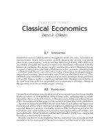
very rapidwhenthe bivalve is first exposed and then levels off, sometimes requiring extensive time
periods foranequilibriumstate to be reached (Figure8.1a). Asimilar trend(Figure8.1b) is
observedfor theeliminationprocess, which may be rapid at first and then leveloff,some
compounds never being fully eliminated (i.e., somecompounds with half-lives of 20 years).
Uptake and elimination rates for both HOCs and metalscan be determined through field and/or
laboratory studies. One potential concern in these types of studies is the possibility that the bivalves
stop siphoning. Although this is morelikely to influence studies of shorter duration, it shouldbe
taken into consideration when analyzing the data.Atypical uptake/elimination experiment consists
of “clean” bivalves (referenced or depuratedprior to commencement of the study) exposedtoa
constant chemical concentration in water,and sampledatincreasing time intervals, to determinethe
chemical concentrations in tissue over time. For example, bivalves can be collected from arela-
tivelyuncontaminated field reference site, and deployed at acontaminated field site, or brought
back to the laboratory for contaminant exposure. After sufficient exposure time,the organisms are
removed and placed in clean water for measurement of the elimination (depuration) rate of the
compounds. In the natural environment, elimination of certain chemicals might require extensive
time periods. In locationswhere exposure levels areconstantorincreasing, bivalvesmay not
eliminate the chemicals. In manyinstances, bivalves will accumulate contaminants to levels sig-
nificantly higher than those in the water column. This can pose toxicity risks to the mussel and
predatoryanimals or canresultinbiomagnificationand subsequent increases in contaminant
concentrations progressively up the food web.
B IOCONCENTRATION

The accumulation of contaminants from the water column by bivalves is referred to as “bioconcen-
tration.” Bioconcentration is defined as the partitioningofacontaminant from an aqueous phase
into an organism andwill occurwhenthe contaminantuptakerate is greaterthanthatfor
Freshwater BivalveEcotoxicology170
4284X—CHAPTER 8—17/10/2006—14:54—KARTHIA—XML MODEL C–pp. 169–213
© 2007 by the Society of Environmental Toxicology and Chemistry (SETAC)
elimination. Typically, thisleads to high concentrations of chemicals in bivalve tissues. For HOCs,
partitioning generally occurs betweenthe dissolved phase of the water and the organism lipid. The
most basic example of partitioning is defined as the octanol–water partition coefficient, or K
ow
:
K
ow
Z ½ contaminant
octanol
= ½ contaminant
water
The K
ow
is ameasurement of achemical’s affinity for octanolversus water. In manycases,
octanol is used as asurrogatefor the organism lipid. Achemical with alesser K
ow
value(less than
100) will partition less into the lipid than achemical with agreater K
ow
(greater than 1,000).This type
of partitioning will occur between the aqueousphase and bivalve lipid until asteady-state condition
has been reached (i.e., the concentration in the organism relative to the exposure system is unchan-
ging with time). Once steady-state or equilibrium has been reached, it is generally referred to as
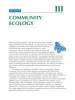
“equilibriumpartitioning.” In asimplesystem, equilibriumpartitioning can be modeledby

comparing theaffinities (i.e.,solubilitiesand fugacities) of achemical forbivalvelipid versus
water (Figure 8.2). To determine the extent of bioconcentration of achemical in tissues, a“biocon-
centration factor”orBCF can be calculated. TheBCF is defined as the pollutant concentration in the
bivalveltissue ( C
tissue
)divided by the dissolved aqueouspollutant concentration ( C
water
)atsteady-
state:
BCF Z C
tissue
= C
water
0
2
4
6
8
10
12
14
0100
(a)
(b)
200 300 400 500
0100 200 300 400 500
Time (hours)
Mussel concentration (ng/g)
0
2

4
6
8
10
12
14
Time (hours)
Mussel Concentration (ng/g)
FIGURE 8.1 Hypothetical uptake (a) and elimination (b) curve in afreshwater mussel. Note in this example,
the rapid uptake that initially occurs, followed by aleveling offofthe concentration of the contaminant in
mussel tissue. The leveling offisconsidered steady-state and, in this example, is reached following about
100 hours of exposure. The rate of elimination is also rapid and is essentially the reverse of the uptake curve.
When placed in clean water, the mussels initially depurate the contaminant rapidly from their tissues and then
reach aplateau, where no further elimination occurs on this time scale.
Toxicokinetics of Environmental Contaminants in Freshwater Bivalves 171
4284X—CHAPTER 8—17/10/2006—14:54—KARTHIA—XML MODEL C–pp. 169–213
© 2007 by the Society of Environmental Toxicology and Chemistry (SETAC)
TheBCF can alsobedetermined by dividing the empirically derived contaminantuptake rate
constant ( k
1
)bythe empirically derived elimination rate constant ( k
2
):
BCF Z k
1
= k
2
In general,the BCF is related to the hydrophobic character of the contaminant. In this way, BCF
values typically correlate in alinear fashion to K
ow

values (Geyer et al. 1982; Mackay 1982; Hawker
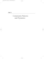
and Connell1986; Pruell et al. 1986; Schuurmann and Klein 1988; Thorsen2003)(Figure8.3).
In many cases, asteady state bioconcentration regression equationcan be developed by linearly
regressing alog BCF versusalog K
ow
plot. The resulting equation for the linetakes the form of
log BCF Z m log K
ow
C b
where m and b are the slope and y -interceptofthe line, respectively. This equation can modelthe
bioconcentrationofhydrophobic organic pollutants by bivalves and can be used to predict aqueous
exposure concentrations.
C
water-
dissolved
C
mussel
C
water-
particulate
FIGURE 8.2 Diagram of theequilibriumpartitioning approach.The hydrophobic organiccontaminant
partitions between the dissolved phase in the water column, the particulate phase in the water column, and
the mussel lipid/tissues. According to Le Chaltelier’s principle, when asystem at equilibrium is disrupted
(e.g., contaminantremoved from particulatephase by amussel),itwillshift to re-establish equilibrium
(e.g.,systemresponds to change by contaminant fromdissolved phase binding to particulatephase).
This model assumes all rates are relatively rapid.
y =1.024 x − 1.8183
R
2
=0.8741

0
1
2
3
4
5
6
3456
log K
ow
log BCF
7
FIGURE 8.3 Example of alinear regression plot of log BCF versus log K
ow
,based on empirical data (From
Thorsen, W. A., Bioavailability of particulate-sorbed polycyclic aromatic hydrocarbons, PhD Thesis, North
Carolina State Univ., Raleigh, NC, 2003). Linear regression has been performed and the resultant regression
equation takes the form: log BCFZ m log K
ow
C b .This regression equation (through simple mathematical
procedures) can be used to predict aqueous exposure concentrations based on tissue residues.
Freshwater BivalveEcotoxicology172
4284X—CHAPTER 8—17/10/2006—14:54—KARTHIA—XML MODEL C–pp. 169–213
© 2007 by the Society of Environmental Toxicology and Chemistry (SETAC)
The “partitioning” of metals, however, generally refers to the adsorption of metalsonto active
sites in/on target tissues, such as anionic sites on bivalve gills (Kramer et al. 1997;Marigomez et al.
2002), rather than absorption into abivalve lipid. Abioconcentration factor, though slightly less
utilitarian than for HOCs due to very slow uptake rate constants, can similarly be computed by
BCF
metal

Z C
tissue
= C
water
where C
tissue
is the moles of metal per gram of soft weight tissue and C
water
is the moles of metal
dissolved per mL (or L) of water. This BCF value must also be calculated when the system has
reached steady-state. More complexequations existfor predicting bioconcentration (and uptake,
elimination rates) whenasystem is not at steady state and are discussedelsewhere (Russell and
Gobas 1989; Butte 1991). Thebioconcentration of metals is affected by many factors, including
water pH, hardness, alkalinity, conductivity, and dissolved organic and inorganic matter, which will
be discussed in following sections.
B IOACCUMULATION
While bioconcentration refers only to the uptake of chemicals directly from the water, the term
bioaccumulation does not differentiate betweenuptakemedia and includeschemical accumulation
into organisms from both abiotic (i.e., water and sediment) and biotic (i.e., food) sources. For
example, bivalves canbioaccumulate chemicals andmetals from thewatercolumnand the
sediment phase in the natural environment.Typically, scientists may model this relationship by
calculating either abioaccumulation factor (BAF) or abiota-sediment accumulation factor (BSAF).
The BAF includesexposure due to water and food sources, whereasthe BSAF (onlyused for
HOCs) models the partitioning/association of achemical betweenthe lipid phasesinthe organism
and the sediment, where the sediment “lipid”phase is considered to be organic carbon. The BAF is
represented by
BAF Z C
tissue
= C
food

C C
water
C C
other exposures
whereasthe BSAF is mathematically defined as
BSAF Z ð C
tissue
= lipid fractionÞ = ð C
sediment
= organic carbon fractionÞ
where the chemical concentration in the bivalve ( C
tissue
)and sediment ( C
sediment
)are normalized
to the mass fraction of organism lipid and sediment organic carbon, respectively. Similar to the
BCF calculation, aBSAF valueiscalculated when the chemical has reached asteady-state
within the studysystem. Theoretically, BSAF values will equal unity or one. However, BSAF
values may be less than one if the bivalve metabolizes the chemical or the system has not
reached steady-state (chemicals may not be fully available to the organism due to very slow
desorption or very strong binding).BSAF values can alsobegreater than one because organic
carbon is generally less“lipid-like” than the organism lipid due to hydrophilic components
of natural organic matter (DiToroetal. 1991).The calculationofBSAFvalues canlend
informationabout aparticular chemical’s bioavailability(see Bioavailabilityand Biotic
LigandModels).
Metalsdonot interact with organisms in the environment in the same way that HOCs do. As
previously mentioned, while HOCsgenerally partition ( absorb) into the lipid phase of abivalve,
metals adsorb to the gill and other anionic sites on tissue surfacesorare actively transported via
membranepumps.For example, metals such as cadmiumcan enter abivalvebybinding to
Toxicokinetics of Environmental Contaminants in Freshwater Bivalves 173

4284X—CHAPTER 8—17/10/2006—14:54—KARTHIA—XML MODEL C–pp. 169–213
© 2007 by the Society of Environmental Toxicology and Chemistry (SETAC)
membrane transport ligands.Bioaccumulation of metals, including filtration of water and ingestion
of food particles, in bivalves can be similarly measured through the use of aBAF:
BAF Z C
tissue
= C
water; dissolved
Bioaccumulation factors for metalsare more difficult to interpret than for organics because the
interactions between atarget site (biological organism) and the metal are complicated by compe-
tition for binding sites and many moreenvironmental variables than simply dissolved or particulate
organic carbon. For all chemicals and metals, bioaccumulation is the balance betweenall means of
chemical uptake and all means of elimination.
M ETABOLISM AND B IOTRANSFORMATION
For those contaminants that bivalvesare capable of metabolizing, BCF, BAF, and BSAFvalues
will be decreased. In general, the lesser metabolic capacities in bivalvesmakes them adequate
sentinels of aquatic environmental pollution (James 1989); however, bivalveshave been shown to
metabolize certain classes of compounds better than others. For example, mussels possess only
minimal abilities to biotransform PAHs, and therefore, are good sentinels of the accumulation of
PAHs.Somemarinemussels ( M. edulis), however,havebeenshowntometabolizethe PCB,
hexachlorobiphenyl (HCBP) (Bauer, Weigelt, and Ernst 1989), and therefore, will exhibit lower
BCF values. Additionally, bivalves have been showntopossess detoxification systems including
lowmolecular weight proteins like metallothionein (MT) andlysosomal granules that make
metals complexand chelate, therebyalteringthe metaluptake/distribution/elimination
kinetics (Naimo 1995;Tessier andBlais 1996; Vesk andByrne 1999; Byrne andVesk2000;
Baudrimont et al. 2002).
B IOAVAILABILITY AND B IOTIC L IGAND M ODELS
Underlying all of the previous concepts is the notion of bioavailability. Bioavailabilitycan be
defined as thepercentageofachemical fullyavailable foruptakebyanorganism.Different
chemicals and inorganiccontaminants have uniquebioavailabilites, which will depend on many

factorsincluding water conditions such as hardness, pH, temperature, and turbidity, as well as the
physical–chemical characteristics of the compound such as water solubility, vapor pressure, and
speciation (ionic state). For example, chemicals that exhibit very low water solubilities readily sorb
to organic carbon phasesinthe water column, such as particulate or dissolved organic carbon (POC,
DOC).The rate of desorptionand co-occurrence of themussel with theparticle(s) partially
determines the chemical’s bioavailability. If the rate of desorption is rapid relative to the co-occur-
renceofthe particle and the organism, the chemical may be fully bioavailable. However, if the rate
of desorption is very slow,the chemical maynot be readilyavailable.HOCsmay frequently
become associated with naturalorganic matter in theaqueous andsedimentphases, whereas
metals may become complexed to various organic (DOC) and inorganiccompounds present in
the water such as calcium and potassium carbonates (CaCO
3
,KCO
3
).
Thebioavailability of achemical is important to understand both to ensure the protectionof
aquatic organismsand to implementeffectiveand cost-efficient remediationtechniques. This
is particularly important because underpredictions of toxicity can result in unacceptable risks to
organisms, whereasoverpredictions of toxicity canrequire costly practicesfor clean-up. For
instance, bivalve tissue burdens are traditionally compared directly to total aqueousorsediment-
contaminant concentrations,without regard for the bioavailable fraction. This method can over-
predict the actual exposure concentrations bivalves (and other aquatic organisms) receive and may
result in costly, yet ineffective, remediation of asite. Moreover, sediment concentrations of total
Freshwater BivalveEcotoxicology174
4284X—CHAPTER 8—17/10/2006—14:54—KARTHIA—XML MODEL C–pp. 169–213
© 2007 by the Society of Environmental Toxicology and Chemistry (SETAC)
metal do notalways correlate well with bivalve tissue burdens. Rather, it may be the speciation of
the metal (e.g., Hg
2 C
versus CH

3
Hg),orratio of metal concentration to the amountofacid-volatile
sulfate in the sediment (DiToro et al. 1992), that best determines the metal concentration in and
subsequent toxicity to the bivalve. One can see the problemsthat may arise when regulatory and
remediation techniques are based on incorrect assessmentsofchemical bioavailability.
HYDROPHOBIC ORGANIC CONTAMINANTS
U PTAKE
As previously stated, HOCs primarily partition into abivalve lipid, which is considered essentially an
“infinite sink” whereby saturation of the pool does not occur. Theuptake of ahydrophobic organic
chemical into bivalve tissues can be defined mathematically as
d C
tissue
= d t Z k
1
C
water
K k
2
C
tissue
where d C
tissue
/dt is the change in bivalve contaminant concentration over change in time ( t ), k
1
is the
uptake rate constant of the chemical, C
water
is the aqueouschemical concentration, k
2
is the elimin-

ation rate (see Elimination), and C
tissue
is the concentration of chemical in the bivalve (see Landrum,
Lee, and Lydy 1992 for areview of toxicokinetic models). If the concentration of the pollutant in the
water column changes, this change will be mirrored in the bivalve over several days to weeks. This
processisconsidered first-order on anatural log(ln)basis. By integration,the above equation
becomes
C
tissue
Z ð k
1
= k
2
Þ C
water
ð 1 K e
K k
2
t
Þ :
Bivalves primarily take up HOCs directly from the water column (Thomann and Komlos 1999;
Birdsall, Kukor,and Cheney 2001) through theirgills,although some studies have suggested
additional chemical inputs from dietaryexposure (Brieger and Hunter 1993; Gossiaux, Landrum,
and Fisher 1996; Bjork and Gilek 1997; Raikow and Hamilton 2001), and direct sediment ingestion
via pedal feeding mechanisms (McMahon and Bogan 2001; Raikow and Hamilton 2001). There is
debate in the literature over the relative contribution of each of these uptake routes; however, it should
be noted that once the system has attained steady-state (dC /dt Z 0), the route of contaminant exposure
is irrelevant(Di Toro et al. 1991). Becauseoftheir minimal metabolic capabilitiesfor metabolizing
the majority of HOCs (Farrington et al. 1983;James 1989), bivalves accumulatethesecontaminants
to high levels in their lipid tissues, which can often reach manyorders of magnitude greater than the

corresponding concentrations in water or sediment phases. Despite the common use of freshwater
bivalvesfor monitoring aquatic environments, relatively little information is knownregarding HOC
uptake rate constants, comparedwith that for marinebivalves. Moreover, much of the freshwater and
marinedata represent only afew species. For instance, the majority of the freshwater uptake studies
focus on Dreissena polymorpha,whereasthe majority of marineuptake studies use M. edulis.
There are various ranges in reported k
1
values for freshwater bivalves depending on species,and
study variablessuchastemperature,exposureenvironment, mussel size, andlipid content
(Table 8.1a,b;Table 8.2a,b for study summaries, Fisheretal. 1993; Bruner, Fisher, and Landrum
1994; Gossiaux, Landrum, and Fisher1996; Fisheretal. 1999). However, based on the available data,
most k
1
values compare well,with only afew exceptions (Table 8.1a). Many studies demonstrate
initial rapid uptake during initial exposure for both freshwater and marine species (Lee,Sauerheber,
and Benson 1972; Obana et al. 1983; Bjork and Gilek1997; Birdsall, Kukor, and Cheney 2001). For
example, Birdsall, Kukor, and Cheney (2001) reportedrapid uptake of the PAHs naphthalene (N0),
anthracene (AN), and chrysene (C0) by Elliptio complanata gills. Their data demonstrated that the
Toxicokinetics of Environmental Contaminants in Freshwater Bivalves 175
4284X—CHAPTER 8—17/10/2006—14:54—KARTHIA—XML MODEL C–pp. 169–213
© 2007 by the Society of Environmental Toxicology and Chemistry (SETAC)
TABLE 8.1a
Published Uptake and Elimination Rate Constantsfor Various Freshwater and Marine BivalveSpecies as aFunction of Chemical Class
and Water Solubility
Species Chemical Class
a
Log K
ow
k
1

(mL/g day) k
2
(day
L 1
)References
Freshwater
E. complanata PAH (34) 3.37(N0)–7.64(CO) Thorsen (2003)
PAH (38) 3.37(N0)–7.64(CO)
PAH (45) 3.37(N0)–7.64(CO) 0.0400(PE)–
0.2600(26DMN0)
E. complanata PAH (14) 3.92(AC)–6.75(DA) 0.0370(BkF)–0.0217(F0) Gewurtz et al. (2002)
D. polymorpha PCP 5.12 369.0–2,133.00.8600–1.5600Fisher et al. (1999)
C. fluminea PCP 5.12 0.3900–0.4000Basack et al. (1997)
C. leana Pesticides (3)3.22(OX)–4.22(TBC) 24.2(TBC)–338.0(CNF) 0.0450(CNF)–0.0600(TBC)Uno et al. (1997)
D. polymorpha PAH (2) 5.18(PY)–6.04(BaP)672.0(BaP)–32,737.0(BaP) 0.0240–0.3840(BaP) Gossiaux, Landrum, and
Fisher(1996)
PCB (2)5.90(PCP)–6.90(HCBP) 2,280.0(PCP)–
26,448.0(HCBP)
0.0240(HCBP)–
0.1920(PCP)
D. polymorpha TCBT (8)6.73(28)–7.54(25)683.3(52)–848.7(80) 0.0052(27)–0.0226(21)Van Haelst et al. (1996a)
D. polymorpha PCB (36) 5.60(42)–7.36(180) 0.0420(183)–0.1720(64) Morrison et al. (1995)
A. anatina PCP 5.12 Makelaand Oikari (1995)
P. complanata PCP 5.12
D. polymorpha PAH (2) 5.18(PY)–6.04(BaP)7,680.0(PY)–31,200.0(BaP)0.1920(BaP)–0.5760(PY) Bruner, Fisher, and Landrum
(1994)
PCB (2)5.9(TCBP)–6.9(HCBP) 9,120.0–40,320.0(HCBP) 0.1200(HCBP)–
0.5040(TCBP)
D. polymorpha PAH (2) 5.18(PY)–6.04(BaP)10,272.0(PY)–
20,112.0(BaP)

0.0090(PY, BaP) Fisher et al. (1993)
PCB (2)5.90(TCBP)–6.90(HCBP) 4,008.0–25,752.0(HCBP) 0.0040(HCBP)–
0.0170(TCBP)
OC (1)6.19(DDT)2,976.0–17,664.0(DDT) 0.0070–0.0080(DDT)
D. polymorpha PCB (2)6.36(77)–7.42(169) 551.0(77)–1,480.0(169) 0.0340(169)–0.0350(77) Briegerand Hunter (1993)
E. complanata HCB, OCS 5.45(HCB)–6.29(OCS) 650.0(HCB)–1,010.0(OCS) 0.4100(HCB)–0.1600(OCS) Russell andGobas (1989)
Freshwater BivalveEcotoxicology176
4284X—CHAPTER 8—17/10/2006—14:54—KARTHIA—XML MODEL C–pp. 169–213
© 2007 by the Society of Environmental Toxicology and Chemistry (SETAC)
Marine
M. edulis PCB (3)5.67(31)–6.92(153) 2,160.0–168,000.0(153)0.0288(153)–0.1368(31) Bjork and Gilek (1997)
C. virginica PAH (7) 4.57(P0)–7.0(IP) 0.0200(FL)–0.0770(BaP) Sericano, Wade, and Brooks
(1996)
PCB (9)0.0053(149)–0.01540(110)
M. mercenaria PAH (9) 3.37(N0)–6.04(BaP) ND over 45 days Tanacredi and Cardenas
(1991)
C. virginica PAH (14) 4.57(P0)–6.50(BghiF) 330.0(P0)–2,365.0(MPY) 0.0090(BF)–0.1180(FL)Benderetal. (1988)
M. mercenaria PAH (14) 4.57(P0)–6.50(BghiF) 187.0(MP0)–2,842.0(BaA) 0.0870(BaP)–0.2130(FL)
M. edulis PAH (6) 3.90–6.100.0231(FL)–0.0578(BkF)Pruell et al. (1986)
PCB (4)5.00–6.600.0150(HCBP)–
0.0420(TCBP)
Short-necked clam PAH (4) 4.42(D0)–5.89(D3) 0.1000(D3)–0.2400(D2)Ogata et al. (1984)
Oyster PAH (4) 4.42(D0)–5.89(D3)
Mussel PAH (4) 4.42(D0)–5.89(D3)
Abbreviations:AC=acenaphthene; BaP=beazo[a]pyrene; BghiF=benzo[ghi]fluoranthene;BkF=benzo[k]fluoranthene; C0=chrysene; CNF=chlornitrofen; D0=dibenzothiophene; DA=diben-
zanthracene; D2=dimethyldibenzothiophene;D3=trimethyldibenzothiophene; 2,6DMN0=2,6-dimethylnaphthalene; F0=fluorene; FL=fluoranthene; HCB=hexachlorobenzene;
IP=indenopyrene; N0=naphthalene; OC=organochlorine; OCS=octachlorostyrene;OX=oxadiazon;PAH=polycyclic aromatic hydrocarbon; PCB=polychlorinated biphenyl (number in
parenthesesreferstoIUPAC PCB congener); PCP=pentachlorophenol; PE=perylene; PY=pyrene; TBC=thiobencarb; TCBP=tetrachlorobiphenyl; TCBT=tetrachlorobenzyltoluene.
a
Number in parentheses referstototal number of chemicals studied within the chemical class.

Toxicokinetics of Environmental Contaminants in Freshwater Bivalves 177
4284X—CHAPTER 8—17/10/2006—14:54—KARTHIA—XML MODEL C–pp. 169–213
© 2007 by the Society of Environmental Toxicology and Chemistry (SETAC)
TABLE 8.1b
Published Solubility Values, Bioconcentration Factors, and Half-Livesfor Various Freshwater and Marine Bivalves as aFunction of
Chemical Class
Species Chemical Class log K
ow
log BCF T
1/2
(days) References
Freshwater
E. complanata PAH (34) 3.37(N0)–7.64(CO) 1.54(N0)–4.66(PE)Thorsen (2003)
PAH (38) 3.37(N0)–7.64(CO) 1.90(N0)–5.20(CO)
PAH (45) 3.37(N0)–7.64(CO) 1.60(AN)–5.51(C4) 2.60(26DMN0)–16.50(PE)
E. complanata PAH (14) 3.92(AC)–6.75(DA) 3.20(F0)–18.70(BkF) Gewurtz et al. (2002)
D. polymorpha PCP 5.12 2.60–3.10 0.44–0.81Fisher et al. (1999)
Corbicula fluminea PCP 5.12 1.73–1.78Basack et al. (1997)
C. leana Pesticides (3)3.22(OX)–4.22(TBC) 2.34(OX)–4.14(CNF)11.60(TBC)–15.40(CNF)Uno et al. (1997)
D. polymorpha PAH (2) 5.18(PY)–6.04(BaP)4.34(PY)–5.43(BaP) 1.75(BaP)–28.80(BaP) Gossiaux, Landrum, and
Fisher(1996)
PCB (2)5.90(PCP)–6.90(HCBP) 4.00(PCP)–5.74(HCBP) 3.60(PCP)–28.80(HCBP)
D. polymorpha TCBT (8)6.73(28)–7.54(25)4.43(80)–5.19(27)18.60(80)–71.80(22)Van Haelst et al. (1996a,
1996b)
D. polymorpha PCB (36) 5.60(42)–7.36(180) 4.00(64)–16.50(183) Morrison et al. (1995)
A. anatina PCP 5.12 1.90–2.10 Makelaand Oikari (1995)
P. complanata PCP 5.12 1.80–1.90
D. polymorpha PAH (2) 5.18(PY)–6.04(BaP)4.11(PY)–4.92(BaP) 1.20(PY)–3.60(BaP) Bruner, Fisher, and Landrum
(1994)
PCB (2)5.90(TCBP)–6.90(HCBP) 4.32(TCBP)–5.38(HCBP)1.40(TCBP)–5.80(HCBP)

D. polymorpha PAH (2) 5.18(PY)–6.04(BaP)4.65(PY)–4.88(BaP) 2.60(BaP)–3.00(PY) Fisher et al. (1993)
PCB (2)5.90(TCBP)–6.90(HCBP) 4.62(HCBP)–5.43(HCBP) 1.70(TCBP)–7.20(HCBP)
OC (1)6.19(DDT)4.72–5.03(DDT) 3.60–4.30(DDT)
D. polymorpha PCB (2)6.36(77)–7.42(169) 4.02(77)–4.45(169) 19.80(77)–20.40(169) Briegerand Hunter (1993)
E. complanata HCB, OCS 5.45(HCB)–6.29(OCS) 3.56(HCB)–4.16(OCS) 1.70(HCB)–4.30(OCS) Russell andGobas (1989)
Marine
M. edulis PCB (3)5.67(31)–6.92(153) 4.70(49)–6.80(153)BAFs 5.00(31)–24.20(153) Bjork and Gilek (1997)
C. virginica PAH (7) 4.57(P0)–7.00(IP)9.00(BaP)–26.00(FL) Sericano, Wade, and Brooks
(1996)
Freshwater BivalveEcotoxicology178
4284X—CHAPTER 8—17/10/2006—14:54—KARTHIA—XML MODEL C–pp. 169–213
© 2007 by the Society of Environmental Toxicology and Chemistry (SETAC)
PCB (9)22.00(26)–130.00(149)
M. edulis PCB (21) 5.07(8)–7.42(169) About 5.30–7.10 Bergen,Nelson, and Pruell
(1996)
C. virginica PAH (14) 4.57(P0)–6.50(BghiF) 3.20(P0)–4.90(BF) 5.90(FL)–77.00(BF) Benderetal. (1988)
M. mercenaria PAH (14) 4.57(P0)–6.50(BghiF) 3.20(MP0)–4.40(BghiF) 3.30(FL)–8.00(BaP)
M. edulis PAH (6) 3.90–6.102.00–4.40 11.90–29.80 Pruell et al. (1986)
PCB (4)5.00–6.604.50–6.60 16.30–45.60
Short-necked clam PAH (4) 4.42(D0)–5.89(D3) 2.17(D0)–2.58(D3) 2.90(D2)–6.90(D3) Ogata et al. (1984)
Oyster PAH (4) 4.42(D0)–5.89(D3) 3.12(D0)–4.45(D3)
Mussel PAH (4) 4.42(D0)–5.89(D3) 2.87(D1)–3.62(D3)
Abbreviations:AC=acenaphthene; BaP=beazo[a]pyrene; BghiF=benzo[ghi]fluoranthene;BkF=benzo[k]fluoranthene; C0=chrysene; CNF=chlornitrofen; D0=dibenzothiophene; DA=diben-
zanthracene; D2=dimethyldibenzothiophene;D3=trimethyldibenzothiophene;2,6DMN0=2,6-dimethylnaphthalene;F0=fluorene; FL=fluoranthene; HCB=hexachlorobenzene;
IP=indenopyrene; N0=naphthalene; OC=organochlorine; OCS=octachlorostyrene;OX=oxadiazon;PAH=polycyclic aromatic hydrocarbon; PCB=polychlorinated biphenyl (number in
parenthesesreferstoIUPAC PCB congener); PCP=pentachlorophenol; PE=perylene; PY=pyrene; TBC=thiobencarb; TCBP=tetrachlorobiphenyl; TCBT=tetrachlorobenzyltoluene.
Toxicokinetics of Environmental Contaminants in Freshwater Bivalves 179
4284X—CHAPTER 8—17/10/2006—14:54—KARTHIA—XML MODEL C–pp. 169–213
© 2007 by the Society of Environmental Toxicology and Chemistry (SETAC)
TABLE 8.2a

SummaryofExposure andTest Duration for Toxicokinetic Studies in the Peer-Reviewed
Reference with Various HOC Classes and Freshwater and MarineBivalves
Species ExposureChemical Class Duration References
Freshwater
D. polymorpha Reeders, Bij de Vaate,
and Slim (1989)
E. complanata HCB, OCS Russel and Gobas
(1989)
D. polymorpha PAH, PCB Fisher et al. (1993)
D. polymorpha Water, sediment,
food
PCB, 321- to 100-day
exposure, rapid
elemination
Brieger and Hunter
(1993)
D. polymorpha Water only PAH, PCB 6-hour uptake Bruner,Fisher, and
Landrum (1994)
A. anatina, P.
complanata
Water only PCP Steady-state reached
in 16 h
Makela and Oikari
(1995)
D. polymorpha Water and field PCB, 36 2-day exposure,
16-day elimination
Morrison et al. (1995)
D. polymorpha Water only PAH, PCB 6-hour uptake, 15-day
elimination
Gossiaux, Landrum,

and Fisher (1996)
D. polymorpha Water only PCBs, OCs Chevreuil et al. (1996)
D. polymorpha Water only TCBTs, 821-day uptake, no
steady-state
reached
Van Halest et al.
(1996a, 1996b)
C. flumina Water only PCP 96-hour uptake,
72-hour elimination
Basack et al. (1997)
C. leana River water Pesticides 14-day uptake, 15-day
elimination
Uno et al. (1997)
D. polymorpha Water only PAH, PCB Fisher et al. (1999)
E. complanata Water only PAH, pesticides Used excised gills Birdsall, Kukor, and
Cheney (2001)
E. complanata Water only PAH, 14 5-day uptake, 32-day
elimination
Gewurtz et al. (2002)
E. complanata Water only and
sediment
PAH, 34–48 20-day exposure,
20-day elimination
Thorsen(2003)
Marine
Oysters No. 2Fuel oil 60-day uptake, 180-
day elimination
Blumer, Souza, and
Sass (1970)
M. edulis Water only PAH Lee, Sauerheber, and

Benson (1972)
Oysters No. 2Fuel oil 49-day uptake, 28-day
elimination
Stegman and Teal
(1973)
M. edulis PAH Clark and Findley
(1975)
Mussels PAH, BaP Dunn and Stich
(1976)
Clams Chronic pollution 120-day elimination Boehm and Quinn
(1977)
M. edulis PAHs Hansen et al. (1978)
(continued)
Freshwater BivalveEcotoxicology180
4284X—CHAPTER 8—17/10/2006—14:54—KARTHIA—XML MODEL C–pp. 169–213
© 2007 by the Society of Environmental Toxicology and Chemistry (SETAC)
average uptake of AN (log K
ow
4.54) and C0 (log K
ow
5.86) was similar, and both were greater than
that for N0 (log K
ow
3.37), which was explained by its lower lipid affinity.
Differencesin k
1
can be observed whencomparing the sameanalyte among studies,aswell as
when comparing different analytes with similar physico-chemical parameters. However, with afew
exceptions, the differencesappeartoberelatively small, considering the many variables that can
exist betweenstudies.For example, k

1
values measured for benzo(a)pyrene (BaP) and HCBP in
both the field and laboratory over the course of three years and at different temperatures (5–248 C)
in D. polymorpha compare well (Table 8.1a). Specifically, for BaPthe range of uptake rates is from
9,960 to 32,736 mL/g day, afactor of 3difference.The differences betweenhighest and lowest
update rate constants for HCBP, pentachlorophenol (PCP), and pyrene(PY) are even less, at factors
of 2.0, 2.6, and 2.0, respectively. Data from two collection timepoints have been omitted for this
comparison due to very low uptake rate constants, which the authors believedwas from over-
wintered musselsexperiencing stress (bothoccurredfor musselscollectedat48 Cinthe field;
however,when mussels were fed while being acclimated to 4 8 Cinthe laboratory, these effects
were not observed) (Gossiaux, Landrum, and Fisher 1996). Therefore, it is important to consider
that larger differencescan occur based on the physiologicalstate of the organism. Laboratory-
derived k
1
sfor PCP increased from 3,960 mL/g day at 4 8 Cto5,928 mL/g day at 158 C, whereas
field-derived k
1
sshowed even less difference with amore dramatic temperature increase from 4to
248 C(3,240 versus 2,640 mL/g day, respectively) (Gossiaux, Landrum, and Fisher 1996). These
TABLE 8.2a (Continued)
Species ExposureChemical Class Duration References
Ostrea edulis Flow-through system PAH, N0 Riley et al. (1981)
Tapes japonica Water and field PAH, 97-to14-day exposure Obana et al. (1983)
Clam, oyster, mussel Water only PAH, D0-D3 Ogata et al. (1984)
Oysters PAH 15-day uptake Pittinger et al. (1985)
M. edulis Sediment dosed PAH, PCB 40-day uptake, 40-day
elimination
Pruell et al. (1986)
M. edulis PAHs Broman and Ganning
(1986)

Mutiple aquatic
organisms
Multiple HOCs Hawker and Connell
(1986)
P. viridis Field PCB, 54 17-day uptake, 32-day
elimination
Tanabe, Tatsukawa,
and Phillips (1987)
C. virginica,
M. mercenaria
Field and laboratory PAH, 14 28-day uptake, 28-day
elimination
Bender et al. (1988)
Clams PAH 2-day uptake, 45-day
elimination
Tanacredi and
Cardenas (1991)
Oysters Water only PCB, 77 Sericano et al. (1992)
M. edulis Field PCBs 28-day exposure Bergen, Nelson, and
Pruell (1996)
M. edulis Water and food PCBs Gilek, Bjork, and
Naef (1996)
M. edulis Water and algae PAH, P0 20-day exposure,
14-day elimination
Bjork and Gilek
(1996)
C. virginica Field PAH, PCB 28- to 50-day uptake,
50-day elimination
Sericano, Wade, and
Brooks (1996)

M. edulis Water and food PBCs Bjork and Gilek
(1997)
Toxicokinetics of Environmental Contaminants in Freshwater Bivalves 181
4284X—CHAPTER 8—17/10/2006—14:54—KARTHIA—XML MODEL C–pp. 169–213
© 2007 by the Society of Environmental Toxicology and Chemistry (SETAC)
TABLE 8.2b
SummaryofVariables Measured and PrimaryFindingsfor Various Bivalves Published in
the Peer-Reviewed References
Species Variables Measured PrimaryFindings References
Freshwater
D. polymorpha No change in k
1
within a
season, but change between
seasons
Reeders, Bij de Vaate, and
Slim (1989)
E. complanata BCF, k
2
Russell and Gobas (1989)
D. polymorpha k
1
Fisher et al. (1993)
D. polymorpha k
1
, k
2
,BCF/BAF Brieger and Hunter (1993)
D. polymorpha k
1

, k
2
,BCF, T
1/2
k
2
depends on the lipophilicity
of achemical
Bruner, Fisher, and Landrum
(1994)
A. anatina,
P. complanata
BCF Makela and Oikari (1995)
D. polymorpha k
2
, T
95
Morrison et al. (1995)
D. polymorpha k
1
, k
2
,BCF, T
1/2
Temperature effects,
monophasic elimination
Gossiaux, Landrum, and
Fisher (1996)
D. polymorpha Responses to change in
aqueous OC concentrations

within 7days
Chevreuil et al. (1996)
D. polymorpha Bivalves: have MFO but
capabilities are/ fish
Van Haelst et al. (1996b)
D. polymorpha k
1
, k
2
,BCF, T
1/2
Log K
ow
versus k
2
:
independent; mussel lipid
decrease over time
Van Haelst et al. (1996a)
C. flumina k
2
No extensive phase I
metabolism
Basack et al. (1997)
C. leana k
1
, k
2
,BCF Measured pesticide
concentrations in musselsin

rice patties
Uno et al. (1997)
D. polymorpha k
1
, k
2
,BCF, T
1/2
Temperature and pH effects Fisher et al. (1999)
PAH uptake due to partitioning
from water to animal across
gill surface
Thomann and Komlos (1999)
E. complanata Average uptake of ANZ
COO N0
Birdsall, Kukor, and
Cheney (2001)
E. complanata k
2
Linear relationshipbetween
log K
ow
and k
2
Gewurtz et al. (2002)
E. complanata k
2
,BCF, T
1/2
Stressed mussels: lower k

2
sThorsen (2003)
Marine
Oysters Little eliminationafter
180 days
Blumer, Souza, and Sass
(1970)
M. edulis Rapid N0, BaP uptake but no
metabolism; k
2
depends on
lipophilicity of chemical
Lee, Sauerheber, and
Benson (1972)
Oysters Elimination nearly complete
after 28 days
Stegman and Teal (1973)
M. edulis k
2
dependent on chemical
lipophilicity
Clark and Findley (1975)
(continued)
Freshwater BivalveEcotoxicology182
4284X—CHAPTER 8—17/10/2006—14:54—KARTHIA—XML MODEL C–pp. 169–213
© 2007 by the Society of Environmental Toxicology and Chemistry (SETAC)
authors notedthat others (e.g., Reeders, Bij de Vaate,and Slim1989)have documented alack of
substantial change in D. polymorpha filtrationactivity over atemperature range of 5–208 C, which
helpstoexplaintheir data (Gossiaux,Landrum,and Fisher 1996). While k
1

sfor some of
thecompounds in this studyincreased proportionallywithincreasingtemperatureinthe field
Table 8.2b (Continued)
Species Variables Measured PrimaryFindings References
Mussels k
2
dependent on chemical
lipophilicity
Dunn and Stich (1976)
Clams Slight eliminationafter
120 days
Boehm and Quinn (1977)
M. edulis High lipid tissues Z rapid
elimination versus low lipid
tissuesZ slower
elimination: biphasic
Hansen et al. (1978)
O. edulis Gill: primary site: uptakeC
accumulation
Riley et al. (1981)
T. japonica Rapid PAH accumulationObana et al. (1983)
Clam, oyster, mussel k
1
, k
2
,BCF Ogata et al. (1984)
Oysters Analytes below detectionlimit
within 4days of elimination
Pittinger et al. (1985)
M. edulis k

2
,BCF, T
1/2
Slow elimination observed and
k
2
depends on liophilicity of
chemical
Pruell et al. (1986)
M. edulis High lipid tissues Z rapid
elimination versus low lipid
tissuesZ slower
elimination: biphasic
Broman and Ganning (1986)
Mutiple aquatic
organisms
Log BCF vs log K
ow
relationship; k
2
dependent
on chemical lipophilicity
Hawker and Connell (1986)
P. viridis k
2
, T
1/2
, T
90
Rapid uptake, release of lower

K
ow
PCBs
Tanabe, Tatsukawa, and
Phillips (1987)
C. virginica M.
mercenaria
k
1
, k
2
,BCF Clams k
2
[ oyster k
2
Bender et al. (1988)
Clams No eliminationobserved in
45 days
Tanacredi and Cardenas
(1991)
Oysters Equilibrium attained in 30 days Serciano et al. (1992)
M. edulis BCF CoplanarPCBs reach steady-
state faster (7 days) than
nonplanar PCBs (14–
28 days)
Bergen, Nelson, and
Pruell (1996)
M. edulis k
2
Body size affects

bioaccumulation because of
influences on k
1
s
Gilek, Bjork, and Naef (1996)
M. edulis k
2
k
2
unaffected by [POC], and
initial uptake rapid
Bjork and Gilek (1996)
C. virginica k
2
, T
1/2
Sericano, Wade, and
Brooks (1996)
M. edulis k
1
, k
2
,BAF, T
1/2
Physioligically-based model of
bioaccumulation, food
ration affected k
1
,but not k
2

Bjork and Gilek (1997)
Toxicokinetics of Environmental Contaminants in Freshwater Bivalves 183
4284X—CHAPTER 8—17/10/2006—14:54—KARTHIA—XML MODEL C–pp. 169–213
© 2007 by the Society of Environmental Toxicology and Chemistry (SETAC)
(e.g., BaP and HCBP), the trend was not consistently exhibited over the three-year time frame and
ledthe authorstosuggest that uptake kineticsdonot change in aproportionalmannerwith
temperature (Gossiaux,Landrum,and Fisher 1996), at least acrossthe range tested. Although
Reeders,Bij de Vaate, andSlim (1989) reported no significantchangeinuptakerates in
D. polymorpha within aseason, asignificant change betweenseasons was documented.
Variations in uptake rates with D. polymorpha body sizeand lipid content were reportedby
Bruner,Fisher, andLandrum (1994) forHCBP, tetrachlorobiphenyl (TCBP),BaP,and PY.
Theaverage uptake rate constantfor HCBP over varyingmussellipid andsize was
23,680 mL/g day (Bruner,Fisher, and Landrum1994), which compared well with k
1
sreported
by Gossiaux, Landrum, and Fisher(1996) for D. polymorpha over varying temperatures, aver-
aging18,624 mL/g day in the laboratory and 21,000 mL/g day in the field. When varying pH is
considered in combinationwith changing temperatures, differencesin k
1
sincreasebut are still
within afactor of lessthan five on average, which translates into about an order of magnitude
difference in BCF values.The reported field andlaboratory k
1
sin D. polymorpha forPCP
(log K
ow
5.12) are 2,760 and 4,120 mL/gday (Gossiaux, Landrum, and Fisher1996), whereas
thosereported for varying pH (and averaged over temperature) are lower:1,657 (pH 6.5), 1,218
(pH 7.5), and 868 (pH 8.5) (Fisher et al. 1999). Thelesser k
1

smay be due to the dissociable nature
of PCP in the range of ambient pH (pK
a
Z 4.74) or to acombination of effects causedbychanging
pH andtemperature on mussel filtration ratesand subsequent uptakerates.Whenindividual
values are compared, rather than averages, the variation in k
1
is increased. For instance, the
smaller the mussel size (measured in shell length),the faster the uptake rate (Bruner,Fisher,
and Landrum1994). Large (21 mm) zebra mussels with high lipid content (greater than 9%) had
TCBP uptake rate constants of 10,080 mL/g day, whereassmaller (15 mm) but also higher lipid
contentmussels (greater than 9%), hadTCBPuptakerateconstants twicethatofthe larger
mussels at 23,760 mL/g day (Bruner, Fisher, and Landrum1994).
In general, uptake rates were directly proportional to compound K
ow
;as K
ow
increased, k
1
increased as well.For example, as log K
ow
values increased from 5.18 for PY to 6.90 for HCBP,the
averageuptakerateconstantincreased from10,480to23,680mL/gday,respectively.An
additionalstudy reported k
1
sranging from 2,976 to 25,752 mL/g dayin D. polymorpha for
PAHs, PCBs, and OCs (DDT) spanning asimilar log K
ow
range of 5.2–6.7 (Fisher et al. 1993).
This range is comparable to the other k

1
spreviously listed,when values for DDT are omitted
(lowest values). Moreover, k
1
values reported for HCB (hexachlorobenzene)and OCS (octachlor-
ostyrene) in E. complanata also increased with increasing log K
ow
;from 650/day for HCB (log K
ow
5.45) to 1,010/day for OCS (log K
ow
6.29) (Russell and Gobas 1989). However, thesevalues are
substantially less than those reportedfor D. polymorpha.
In contrast to the linear relationship between k
1
and K
ow
reported by some (Russelland Gobas
1989; Bruner, Fisher, and Landrum1994; Gossiaux, Landrum, and Fisher 1996), uptake rates for
eightdifferent TCBT congeners in D. polymorpha were independent of K
ow
(Van Haelstetal.
1996a). As log K
ow
increased from 6.73 (TCBT#28) to 7.54 (TCBT #25), k
1
svaried little, from
772 to 803 mL/gday (Van Haelst et al. 1996a), respectively. However, whenall TCBT congeners
were includedinthe log K
ow

range, the k
1
values demonstrated larger variation and rangedfrom
683.3 to 848.8 mL/gday. This may be partially explained by the high K
ow
values or the decreased
ability of highly hydrophobic compoundstopermeate membranes (Van Haelst et al. 1996a). More-
over, the uptake rates reportedfor D. polymorpha for TCBT congeners are lower than those for
PAHs or PCBs with similar hydrophobicity (see previous values).Uptake rate constantsfor PCB
congener 153 (Bruner, Fisher, and Landrum1994)and TCBT (tetrachorobenzyltoluene)congener
28 (Van Haelstetal. 1996a), which have similar log K
ow
values (6.92 and 6.73, respectively), differ
by as muchasafactor of 50, from as low as 771 mL/g day for TCBT congener 28 (Van Haelst et al.
1996a)tobetween9,120 and 38,592 mL/g day for congener 153 (Bruner,Fisher, and Landrum
1994), both for D. polymorpha.
Freshwater BivalveEcotoxicology184
4284X—CHAPTER 8—17/10/2006—14:54—KARTHIA—XML MODEL C–pp. 169–213
© 2007 by the Society of Environmental Toxicology and Chemistry (SETAC)
Bjork and Gilek(1997) reported k
1
sfor three PCB congeners (PCBs 31, 49,153) in the marine
mussel, M. edulis,that rangedfrom 2,160 (PCB153) to 168,000 mL/g day (PCB153). While the
upperrange is quite large,and is aboutfourtimes greaterthanthe upperrange reported for
D. polymorpha,the freshwatermussel k
1
sare still withintheselimits. The larger k
1
values in
M. edulis are probably due to the addition of contaminated food in the study conducted by Bjork

and Gilek (1997).Incontrast, Ogata et al. (1984) reported k
1
sfor parent and various alkylated
dibenzothiophenes in amarine short-neckedclam, which were significantly less ranging from 33/
day for dibenzothiophene to 66/dayfor dialkylated dibenzothiophene. It should be noted that some
authors (e.g., Ogata et al. 1984; Russell and Gobas1989)have reported k
1
values in reciprocal days,
which is assumed to be equivalent to mL/g day (where 1mL Z 1g). However, this assumption may
not always be valid, which may explain someofthe differencesobserved in k
1
values.
Uptake ratesfor variouspesticides in theAsian clam Corbicula leana (Uno et al.1997)
are muchlower than those reported in D. polymorpha for compounds with similar K
ow
s. While
the log K
ow
for the pesticides thiobencarb, oxadiazon,and chlornitrofen are less than the HOCs, the
uptakerateconstantsare more than proportionallyless, ranging from 24.2 forthiobencarb to
626.0 mL/g day for chlornitrofen in the field and 140 for thiobencarb to 338 mL/g day for chlorni-
trofeninthe laboratory (Uno et al. 1997).The authorsattributed thelow uptakerate(s) for
thiobencarb to atemperature decrease of 2 8 Cover the course of ayear causing slower ventilation
rates in the mussels. In contrast, reports with D. polymorpha show that atemperature range of 208 C
does notcause substantial changesinuptake rates (Reeders, Bij de Vaate,and Slim 1989; Gossiaux,
Landrum, and Fisher1996).The large differences in uptake rates for C. leana versus D. polymorpha
and M. edulis are probably due to acombination of species and chemical differences.
In summary, uptake rate constants were remarkably similar across temperature, season, pH,
chemical, and study variables, although somedifferences were observed, particularly when
comparing chemicals of similar log K

ow
(TCBTs versus PCBs), lowversushighlipid
content,and bivalves of differing size and species. Large variation in k
1
was demonstrated
for stressed mussels (Gossiaux, Landrum, and Fisher 1996), suggesting that bivalve physiology
must be considered whenmeasuring empirical uptake rates or BCFs under adverse conditions
such as very low temperatures. Moreover, k
1
sweregreater forcombined food andwater
exposures (Bjork and Gilek1997). The uptake rate constantsreported in this chapter represent
only those for afew freshwater mussel and clam species, which demonstrates the need for
further research in this area. For instance, while D. polymorpha uptake rate constantsmay not
vary substantially with increases or decreasesintemperature (over a20 8 Crange)(Gossiaux,
Landrum, and Fisher1996), this may not be the case for other freshwater bivalve species
(e.g., Corbicula)(Uno et al. 1997).
B IOCONCENTRATION
Gossiaux, Landrum, and Fisher(1996)reported bioconcentration factorsin D. polymorpha for
BaP(log K
ow
6.04) that rangedfrom4.38 to 5.28 logbioconcentration in field exposures at
temperatures from 4to24 8 C. The BaP log BCF values had asimilar range in the laboratory for
temperatures from 4to20 8 C(4.60 (48 C) to 5.43 (158 C), Table 8.1b). Thelog BCF values for PY
(log K
ow
5.18) in both the field and laboratory ranged from 4.34 to 4.89, over asimilar temperature
range. However, the authors were not convinced that steady-state had been reached due to afactor
of 100 difference betweenBCF values calculated from C
tissue
/ C

water
and those calculated from k
1
/
k
2
.Thisimplies BCF values in reality would be larger than those reported or that the organisms
possess some capacity for metabolism of PY. In comparison, Bruner,Fisher, and Landrum(1994)
reportedsimilar log BCF values also in D. polymorpha for both BaP, ranging from 4.61 to 4.92 and
PY, ranging from 4.11 to 4.54, depending on mussel lipid and size. These values compare well,
especially when considering the variation in temperature, lipid content,and size.
Toxicokinetics of Environmental Contaminants in Freshwater Bivalves 185
4284X—CHAPTER 8—17/10/2006—14:54—KARTHIA—XML MODEL C–pp. 169–213
© 2007 by the Society of Environmental Toxicology and Chemistry (SETAC)
In contrast, log BCF values reportedbyThorsen(2003) for E. complanata are lower for both
PAHs, ranging from 3.50 to 4.66 for BaP, and 2.29 to 3.79 for PY, depending on exposure source
(water-only versus sediment). Thedifferencesbetweenthese data may be partially explained by lipid
content of D. polymorpha and E. complanata; D. polymorpha were generally 7–15% lipid on adry
weight basis(Gossiaux, Landrum, andFisher1996) whereas E. complanata were much lower,
typically3–4%lipid (Thorsen2003).The contributionofalipidcan be partly confirmedby
resultsfrom Bruner, Fisher,and Landrum(1994)who reportedanincrease in BCF values with
subsequent increaseinmussel lipid content.However, this effect was only observed for the higher
K
ow
compounds (HCBP and BaP) and notfor the lower K
ow
compounds (TCBP and PY). While
bivalve BCF values are not traditionally normalized to lipid content,itwould be helpful to report lipid
values for conversion and comparison.The addition of lipid-normalized BCF values may help to
explain variationsinbivalve bioconcentration. Furthermore, log BCF values determined for HCB

and OCS in E. complanata (log K
ow
s5.49 and 6.29, respectively) compare well with those for PAHs
of similar hydrophobicity, rangingfrom 3.56 to 4.16 (e.g., 3.58 and 3.64 for C2-dibenzothiophenes
with log K
ow
5.50,and 4.23 and4.54 forbenzo(e)pyrenewith log K
ow
6.20)(Thorsen2003).
Additionalvariations in BCFs maybefurther explainedbyphysiologicaldifferences between
E. complanata and D. polymorpha,differencesinstudydesign, or acombination of environmental
and physiological factors.
Makela and Oikari(1995) reported BCF values for PCP in two freshwater mussels, Anodonta
anatina and Pseudanodontacomplanata,which range from 1.9 to 2.1 and 1.8 to 1.9, respectively.
These BCF values are much lower than those reported by Gossiaux, Landrum, and Fisher (1996) for
PCP in D. polymorpha,which ranged from 4.00 to 5.27, depending on the studytemperature. In
contrast,log BCFvalues reported forPCP in adifferent study for D. polymorpha with varying
temperature and pH are mid range betweenthose reported for A. anatina, P. complanata (witha
range of 2.60–3.13)(Fisheretal. 1999), and D. polymorpha (4.00–5.27) (Gossiaux, Landrum, and
Fisher1996,Table 8.1b).
Thelog BCF values for HCBP determined in two separate studies on D. polymorpha compare
well,ranging from 4.79 to 5.38 in one study (Bruner,Fisher, and Landrum 1994)and from 5.24 to
5.74 in thesecond (Gossiaux, Landrum,and Fisher 1996). Briegerand Hunter (1993) reported
log BAFvalues for D. polymorpha of 4.02 and4.45 fortwo PCB congeners, 77 (log K
ow
6.36)
and169 (log K
ow
7.42), whichwerelower relativetotheir K
ow

values than thosereported for
similar log K
ow
compounds such as TCBT congener 28 (log K
ow
6.73, log BCF 4.83) (Van Haelst
et al. 1996a, 1996b), HCBP (log K
ow
6.9, log BCF range 4.8–5.7) (Bruner,Fisher, and Landrum
1994; Gossiaux, Landrum, and Fisher1996), and TCBT congener 22 (log K
ow
7.43, log BCF 4.71)
(Van Haelst et al. 1996a, 1996b). These differencesmay simply suggestalack of steady state, as BAF
values wouldbeexpected to be largerthanBCF values from increasedexposure to
contaminated food.
The values of logBCF forvariouspesticides includingchloronitrofen,thiobencarb,and
oxadiazon have been reportedfor C. leana ranging from 2.34 for oxadiazon (log K
ow
3.89) to
4.14 forchlornitrofen in thefield, andfrom3.79for chlornitrofento3.45for thiobencarb
(log K
ow
4.22) in the laboratory (Uno et al. 1997). It should be notedthat the log BCF values for
oxadiazon and thiobencarb increasewith corresponding increases in hydrophobicity.
Bioconcentration factors determined for PAHsin M. edulis (Pruell et al. 1986)and amarine
short-necked clam, oyster, and mussel (Ogata et al. 1984)compare well to those for E. complanata
(Thorsen 2003)but are lessthan thosereportedfor D. polymorpha (see previous comparison between
E. complanata and D. polymorpha). Forexample, across alog K
ow
range of 3.9–6.1, log BCF values

for M. edulis rangedfrom 2.0 to 4.4 (Pruell et al. 1986), whereasacross asimilar log K
ow
range of
3.37–7.60 for E. complanata,log BCF values ranged from 1.5 to 5.2 (Thorsen 2003). Moreover, the
log BCFs reported for dibenzothiophene (D0) in marine clam, oyster, and mussel were 2.17, 3.12,
and 3.13, respectively (Ogata et al. 1984), which are near the range reported for E. complanata of
Freshwater BivalveEcotoxicology186
4284X—CHAPTER 8—17/10/2006—14:54—KARTHIA—XML MODEL C–pp. 169–213
© 2007 by the Society of Environmental Toxicology and Chemistry (SETAC)
2.69–2.93 (Thorsen2003)and similar to thosereportedfor thiobencarb (of similar log K
ow
to D0:
4.22 versus 4.49) in C. leana of 3.25–3.48 (Uno et al. 1997,Table 8.3).
Similar to uptake rateconstant data, empirically derived BCF values generally increase with
increasing K
ow
of the compound (Pruell et al. 1986; Brieger and Hunter 1993; Bruner, Fisher, and
Landrum1994; Gossiaux, Landrum, and Fisher 1996; Thorsen 2003). Forexample, as the log K
ow
is increasedfrom5.18 (PY) to 6.90 (HCBP),the averagelog BCFvaluesfor D. polymorpha
increase from 4.28 to 5.14 (Bruner, Fisher,and Landrum 1994).However, exceptions to this
trend have been observed. The BCFs for compounds with log K
ow
values greater than 6–7 tend
to level offdue to factorssuch as steric hinderance (reduction of membrane permeation), lack of
steady state (very long times required to reach equilibrium), and growth dilution. Van Haelstetal.
(1996a,1996b) foundnocorrelationbetween log BCF values foreight TCBT congeners and
log K
ow
.They suggested that this was due to the small range of log K

ow
(6.73–7.54) compounds
used, as well as the fact that the TCBT congeners all have log K
ow
s O 6(i.e., may be in the linear
part of the curve).
The values of log BCF for PCBs of similar hydrophobicity reportedfor M. edulis were higher
than thosefor PAHs:ranging fromabout5.0 to 5.7for acorresponding PCBlog K
ow
range
of approximately 6.0–7.0 (Pruell et al. 1986). This log BCF range fits withinthat reportedfor
D. polymorpha (Bruner,Fisher, and Landrum 1994; Gossiaux, Landrum, and Fisher1996)for
various PCBs over the same log K
ow
range of 4.0–6.9.However, the differencesbetweenPAH
and PCBs for freshwater musselsappeartobeless pronounced (Bruner, Fisher, and Landrum1994;
Gossiaux, Landrum,and Fisher 1996).Moreover, alinearrelationship betweenlog K
ow
and
log BCF was observed for both PAHs and PCBs in M. edulis (Pruell et al. 1986), E. complanata
(Thorsen 2003), and D. polymorpha (Bruner,Fisher, and Landrum1994). Comparisons of steady-
state bioconcentration regression equations (Table 8.4)demonstrate reasonable agreement in PAH
accumulation, with few exceptions. For example, Pruell et al. (1986) reportedaslope of 0.965 and a
y -interceptof K 1.41 for M. edulis,whereas Thorsen (2003)reported aslope of 0.895and a
y -intercept of K 1.21 ( r
2
Z 0.8325) for E. complanata.However,Ogata et al.(1984) reported
regressionequations with slopes much less than one(0.16 forshort-neckedclams, 0.49 for
oysters, and 0.31 formussels) and positive y -intercepts (1.54, 1.03, 1.63,respectively). The
differencesmay be duetothe fact that theregressionequationsofOgata et al.(1984)were

based on the parent and alkyated homologues of dibenzothiophene only, whereas thoseofPruell
et al. (1986) and Thorsen(2003) were based on data setscontaining greater numbers of PAHs.
These data suggest agood correlation betweenmarineand freshwater BCF values, for M. edulis,
E. complanata,and Mya arenaria.
E LIMINATION
The elimination rateconstant(k
2
)can be calculated from an elimination plot of thelipid
normalized, natural log (ln)ofthe contaminant concentration in bivalve versus time.Inafirst-
order, one-compartment kinetic model, k
2
is the absolutevalueofthe slope of the line, based on the
equation
ln C
tissue
Z K k
2
t C ln C
tissue; 0
where C
tissue,0
is the tissue chemical concentration at elimination time zero (Figure 8.4).
Bivalve elimination rate constants are alsofairly consistent, depending on compound, study,
and species (Table 8.1a). Elimination rates for HOCs are generally much lower than their counter-
part uptake rates but similarly are dependent upon the hydrophobic character of the compounds
(Dunn and Stich 1976; Bruner, Fisher, and Landrum1994; Morrison et al. 1995; Gewurtz et al.
2002; Thorsen et al. 2004a). Gewurtz et al. (2002),who calculated k
2
sfor nine PAHs in
E. complanata,showedvariationfrom 0.037/dayfor benzo(k)fluoranthene (BkF)to0.217/day

Toxicokinetics of Environmental Contaminants in Freshwater Bivalves 187
4284X—CHAPTER 8—17/10/2006—14:54—KARTHIA—XML MODEL C–pp. 169–213
© 2007 by the Society of Environmental Toxicology and Chemistry (SETAC)
TABLE 8.3
Comparison of Bioconcentration/Bioaccumulation Factors and Uptake and Elimination Rate Constants for Similar Solubility HOC
Analytes in the Peer-ReviewedReference
Analyte Log K
ow
Species Log BCF/BAF k
1
(mL/g day) k
2
(day
L 1
)Exposure References
Phenanthrene 4.54 E. complanata 3.02 Water, laboratory Thorsen (2003)
Phenanthrene 4.54 E. complanata 3.44 Sediment,
laboratory
Thorsen (2003)
Phenanthrene 4.57 E. complanata 3.06 Sediment, fieldThorsen (2003)
Phenanthrene 4.57 M. edulis 2.90 Water, food Bjork and
Gilek (1997)
Phenanthrene 4.57 C. virginica 3.21 330
a
0.206 Sediment Bender et al. (1988)
Phenanthrene 4.57 M. mercenaria 3.29 224
a
0.114 Sediment Bender et al. (1988)
Dibenzothiophene 4.49 E. complanata 2.86 Water, laboratory Thorsen (2003)
Dibenzothiophene 4.49 E. complanata 2.69 Sediment,

laboratory
Thorsen (2003)
Dibenzothiophene 4.49 E. complanata 2.93 Sediment, fieldThorsen (2003)
Dibenzothiophene 4.49 Marineclam 2.17 Water Ogata et al. (1984)
Dibenzothiophene 4.49 Marineoyster 3.12 Water Ogata et al. (1984)
Dibenzothiophene 4.49 Marinemussel 3.13 Water Ogata et al. (1984)
Methyldibenzothiophene 4.86 E. complanata 3.43 Water, laboratory Thorsen (2003)
Methyldibenzothiophene 4.86 E. complanata 3.38 Sediment,
laboratory
Thorsen (2003)
Methyldibenzothiophene 4.86 E. complanata 3.07 Sediment, fieldThorsen (2003)
Methyldibenzothiophene 4.86 Marineclam 2.38 Water Ogata et al. (1984)
Methyldibenzothiophene 4.86 Marineoyster 3.40 Water Ogata et al. (1984)
Methyldibenzothiophene 4.86 Marinemussel 3.12 Water Ogata et al. (1984)
Pentachlorophenol 5.20 C. fluminea 0.390–0.400 Water Basack et al. (1997)
Pentachlorophenol 5.20 D. polymorpha 2.60–3.208,856–51,192 0.860–1.560 Water Fisher et al. (1993)
Pentachlorophenol 5.20 D. polymorpha 4.00–4.602,280–5928 0.140–0.190 Water Gossiaux, Landrum,
and Fisher (1996)
Pentachlorophenol 5.20 A. anatine 1.90–2.10Water Makelaand
Oikari (1995)
Freshwater BivalveEcotoxicology188
4284X—CHAPTER 8—17/10/2006—14:55—KARTHIA—XML MODEL C–pp. 169–213
© 2007 by the Society of Environmental Toxicology and Chemistry (SETAC)
Pentachlorophenol 5.20 P. complanata 1.80–1.90Water Makelaand
Oikari (1995)
Benzo[a]pyrene 6.04 D. polymorpha 4.40–5.409,960–32,736 0.020–0.380 Water Gossiaux, Landrum,
and Fisher (1996)
Benzo[a]pyrene 6.04 D. polymorpha 4.60–4.907,920–18,240 0.190–0.410 Water Bruner, Fisher, and
Landrum (1994)
Benzo[a]pyrene 6.04 E. complanata 3.50–4.70Water, sedimentThorsen (2003)

Benzo[a]pyrene 6.04 M. edulis 4.50 0.045 Sediment Pruelletal. (1986)
Benzo[a]pyrene 6.04 C. virginica 4.29 639
a
0.032 Sediment Bender et al. (1988)
Benzo[a]pyrene 6.04 M. mercenaria 3.62 361
a
0.087 Sediment Bender et al. (1988)
Hexachlorobiphenyl 6.90 D. polymorpha 5.20–5.7013,536–26,4480.024–0.960 Water Gossiaux, Landrum,
and Fisher (1996)
Hexachlorobiphenyl 6.90 D. polymorpha 4.80–5.409,120–38,592 0.120–0.680 Water Bruner, Fisher, and
Landrum (1994)
PCB 153 6.90 M. edulis 4.90–6.802,160–168,0000.029 Water, food Bjork and
Gilek (1997)
Indenopyrene 7 Elliptio complanata 4.40–4.56Water, sedimentThorsen (2003)
Dibenzanthracene6.75 Elliptio complanata 4.80–5.20Water, sedimentThorsen (2003)
PCB 169 7.42 Dreissena
polymorpha
4.50 Water, food Brieger and
Hunter (1993)
TCBT 28 6.73 Dreissena
polymorpha
4.80 Water Van Haelst et al.
(1996a)
TCBT 52 7.26 Dreissena
polymorpha
4.50 Water Van Haelst et al.
(1996a)
PCB Mytlius edulis 5.70 Sediment Pruelletal. (1986)
a
Units not specified in reference.

Toxicokinetics of Environmental Contaminants in Freshwater Bivalves 189
4284X—CHAPTER 8—17/10/2006—14:55—KARTHIA—XML MODEL C–pp. 169–213
© 2007 by the Society of Environmental Toxicology and Chemistry (SETAC)
for fluoranthene (FL). An inverse linear relationship was observed betweenanalyte elimination rate
constant and corresponding log K
ow
,which the authors attributed to potential passive elimination of
PAHs(Gewurtz et al. 2002). This type of response is characteristic of monophasic, first-order
elimination, which has also been reported in D. polymorpha for lower K
ow
compounds (Gossiaux,
Landrum, and Fisher1996). Additional k
2
values reportedfor 45 PAHsin E. complanata exposed to
sediment during the uptake phase rangedfrom 0.04 to 0.22/day (Thorsen et al. 2004a). Theauthors
further noted that these elimination rate constantswere less than thosefrom awater-only exposure
studyand suggestedthat it may have been due to increased stress on the musselsfrom an unknown
fungalorbacterial growth,and subsequently, increased handling (Thorsenetal. 2004a). The k
2
values for OCS and HCB in E. complanata rangedfrom 0.16 to 0.41/day and were slightly higher
whencompared to similar log K
ow
PAHs (Russell and Gobas 1989).
Moreover, Gossiaux, Landrum, and Fisher (1996) demonstrated slow elimination rateconstants
for D. polymorpha in field studies, ranging from 0.024 to 0.096/day for HCBP to 0.024 to 0.384/day
for BaP. For the lower hydrophobic compounds in this study (PCP and PY), elimination was rapid
during the first 24 hours and then leveled off, while elimination of HCBP and BaP was minimal over
the first 24 hours, increased during the following 48–168 hours, and then slowed,suggestive of a
biphasic, two-compartment model. These authors, however, classified theelimination
as monophasic.

Furthermore, k
2
sfrom the studies of Gossiaux, Landrum, and Fisher(1996) and Gewurtz et al.
(2002),in D. polymorpha and E. complanata,comparedwell amongHOCs of similar log K
ow
.For
example, Gewurtz et al. (2002) reported a k
2
for PY of 0.144/day, and this is within the range also
TABLE 8.4
Comparison of Steady-State Bioconcentration Regression Equations forOrganic
Contaminants in Freshwater and Marine Mussels
Species
Chemical
Class ExposureSlope y -Intercept r
2
References
Freshwater
E. complanata PAH (34) Water,
laboratory
0.895 K 1.21 0.83 Thorsen (2003)
E. complanata PAH (35) Sediment,field 0.786 K 0.98 0.78 Thorsen (2003)
E. complanata PAH (45) Sediment,lab 0.807 K 1.12 0.73 Thorsen (2003)
Marine
M. edulis PAH (6) Sediment,
laboratory
0.965 K 1.40 Pruell et al.
(1986)
M. edulis Multiple HOCs Water,
laboratory

0.858 K 0.81 0.96 Geyer et al.
(1982)
M. arenaria PAH Water, field 1.097 K 1.54 0.85 Thorsen (2003)
M. arenaria PAH Sediment,field 1.042 K 1.28 0.85 Thorsen (2003)
Multiple
marine
Multiple HOCs 0.844 K 1.23 0.83 Hawker and
Connell
(1986)
Marine clam PAH (4, all D0) Water,
laboratory
0.163 1.52 0.71 Ogata et al.
(1984)
Marine oyster PAH (4, all D0) Water,
laboratory
0.494 1.03 0.62 Ogata et al.
(1984)
Marine mussel PAH (4, all D0) Water,
laboratory
0.311 1.63 0.64 Ogata et al.
(1984)
Freshwater BivalveEcotoxicology190
4284X—CHAPTER 8—17/10/2006—14:55—KARTHIA—XML MODEL C–pp. 169–213
© 2007 by the Society of Environmental Toxicology and Chemistry (SETAC)
reportedfor PY by Gossiaux, Landrum,and Fisher (1996)of0.048–0.312/day. Moreover,
acomparison of dibenzo(a,h)anthracene(DA,log K
ow
6.8, Thorsen2003)and HCBP (log K
ow
6.9, Gossiaux, Landrum, andFisher1996) revealedsimilar k

2
values;0.068/dayfor DA and
0.024–0.096/dayfor HCBP. The k
2
values reported by Bruner,Fisher, and Landrum (1994) were
generally higherthan thoseofGewurtz et al. (2002) and Gossiaux, Landrum, and Fisher(1996).
The k
2
sfor PCP in D. polymorpha were about two to three times less than those reportedfor
Corbicula fluminea ,ranging from 0.140to0.192/dayin D. polymorpha (Bruner, Fisher,and
Landrum 1994)to0.39to0.40/dayin C. fluminea (calculated with data from Basacketal.
1997).However,bothwereless than other k
2
sfor PCPs reported for D. polymorpha,which
ranged from 0.86 to 1.56/day (Fisher et al. 1999), which may have been due to the combination
of changing pH and temperature in that study. However, the overall consistency in k
2
values among
species and studies further suggests that elimination of HOCs is highly dependent upon compound
hydrophobicity,ratherthanother factorssuchasorganismphysiology, andcan be generally
described by afirst order, one-compartment kinetic model (Morrison et al. 1995).
Smaller k
2
values were observed for HOCs with log K
ow
values greater than seven. Van Haelst
et al. (1996a)reportedarange of 0.005–0.037/dayin D. polymorpha for TCBT congeners ranging
in log K
ow
from 6.73 to 7.54, which were approximatelytwo to three times less than otherliterature

k
2
s. For the same K
ow
range, Morrison et al. (1995) demonstrated a k
2
range of 0.042–0.098/dayfor
D. polymorpha,whereas Briegerand Hunter(1993) reportedanelimination rate constantof0.034/day
for PCB congener169 (log K
ow
7.42) in D. polymorpha.There seems to be aplateauing effectof
k
2
values observed forHOCs with log K
ow
sgreater than aboutsix (Morrisonetal. 1995;
Gewurtz et al. 2002;Thorsen et al. 2004a).
The k
2
rates reported in C. leana for the pesticideschlornitrofen and thiobencarb were small
and varied little betweenlaboratory and field studies, ranging from 0.045 (field) to 0.054/day
(lab) for chlornitrofen and 0.049 (lab) to 0.060/day (field) for thiobencarb (Uno et al. 1997).
However, these k
2
values do not follow the trend seen with K
ow
,asthe pesticide K
ow
sare less
than those for the TCBT congeners. These compounds may be metabolized to someextent by

the mussels.
Elimination of HOCs in marine musselswas found to be moderately variable, ranging from
rapid elimination (less than 4days) (Pittinger et al. 1985)tonomeasureable depuration in 45 days
(Tanacredi and Cardenas 1991). However, elimination rate constants for M. edulis (calculated from
y = − 0.0555 x +7.5373
R
2
=0.9157
0
1
2
3
4
5
6
7
8
9
01020
t (d)
ln C mussel
30
FIGURE 8.4 Example of aplot of the natural log (ln) of the lipid normalized mussel tissue concentrations
versus time (Adapted from Thorsen, W. A., 2003). The absolute value of the slope of the linear regression
represents the elimination rate constant, k
2
,for this particular compound. The equation for the line follows the
form: ln C
mt
Z ( k

2
) t C ln C
m0
,where C
mt
is the contaminant concentration in mussel tissue at time t ,and C
m0
is
the contaminant concentration in mussel tissue at time t Z 0(initial).
Toxicokinetics of Environmental Contaminants in Freshwater Bivalves 191
4284X—CHAPTER 8—17/10/2006—14:55—KARTHIA—XML MODEL C–pp. 169–213
© 2007 by the Society of Environmental Toxicology and Chemistry (SETAC)
data in Pruell et al. 1986), ashort-necked clam (speciesnot identified) (Ogata et al. 1984)and
Crassostrea virginica (Sericano, Wade,and Brooks 1996)exhibited similar rangesfor PAHsand
PCBs as those reported for freshwater bivalves. The consistency in regression equations between
freshwater and marinebivalves, PAH, and PCB classes and field and laboratory studies is remark-
able. Awider range in slopes and y -intercepts was observed, however,ifall data for C. virginica
(Easternoyster) and Mercenaria mercenaria (HardClam) were included, which demonstrated
negativeslopes and little depuration in some instances (Tanacredi and Cardenas 1991). Further
researchisrequired for amore robust comparison of freshwater and marine bivalvesand for amore
complete understandingofwhy differencesinelimination rates occur.
A TTAINMENT OF S TEADY -STATE
While most bivalve uptake kinetics are generally rapid for HOCs, there is abroad range of time
requiredtoreachsteady-state (Table 8.2a, b). Forexample, Thorsen (2003) found that steady-state
wasreachedbetweenthe water column andmussel tissuefor most PAHswithin thefirst
24–48 hours of exposure and that all PAHsreached steady-state within 10 days. Likewise, the
uptake kinetics of D. polymorpha are rapid (Bruner,Fisher, and Landrum 1994; Morrison et al.
1995; Gossiaux, Landrum, and Fisher1996), which enables them to reach steady-state quickly
(within afew hours,for lower hydrophobicity chemicals). In contrast, Pruell et al. (1986) reported a
longertime interval to steady-state of 20 days for M. edulis,which may have been due to slow

contaminant desorption from the sediment slurry sourceinto the water. Moreover, Brieger and
Hunter (1993) found that asteady-state for hexachlorobenzene in D. polymorpha required20days,
whereas PCB congener 77 did not appeartoreachsteady-state, even after 30 days of exposure. The
attainment of steady-state will depend on mussel lipid content,metabolic capabilities, physical–
chemical characteristics of the compound (highly hydrophobic compounds may require longer time
periods for equilibrium), and the availability of the chemical. In studies where sediment serves as
the primary exposure media, slow chemical desorption from sediment particles may influence the
time requiredtoreach steady state (e.g., Pruell et al. 1986).
B IOACCUMULATION AND B IOAVAILABILITY
Many studies have demonstrated mussel uptake of HOCsfrom water,contaminated food and
sediment (Augenfield et al. 1982; Brieger and Hunter 1993; Pruell et al. 1993; Bjork and Gilek
1997; Gossiaux, Landrum, and Fisher 1998). The uptake rates of PCB 77 in D. polymorpha
increased when the exposure environment was altered to include food and sediment, in the
followingincreasingorder: water O foodO sediment (Brieger andHunter 1993).Incontrast,
Thorsen (2003) did not observeconsistentdifferences in PAH BCF/BAF values determined
for E. complanata in water-only (BCF) versus sediment(BAF)exposure studies,indicating
that sedimentPAH concentrationswere drivingthe water exposure concentrationsfor
E. complanata.The situationwas similar when E. complanata were allowed to burrow into
the sediment phase in both field and laboratory studies (Thorsen2003). With the exception of
benz(a)anthracene, statisticallysignificant differenceswere not observed in tissue PAH burdens
between D. polymorpha placed in the upper water column versus the sediment surface at a
confineddisposal facility(Roperetal. 1997). However, this maynot be thesituationfor
deposit-feeding bivalves or for bivalves exposed to PCBs, which have generally been shown
to be more bioavailable than PAHs of similar physical–chemical characteristics(Lamoureux and
Brownawell 1999;Kraaij et al. 2002).
While the addition of food and sediment in exposure environments may result in increased
accumulation, thesefactorsmay also result in decreasedbioavailability of HOCsbyserving as
binding agents that sequester them (Kraaij et al. 2002). Many factorscan affect HOC bioavail-
ability, including feeding and digestion mechanismsofthe bivalve,aswell as rates of sorption and
Freshwater BivalveEcotoxicology192

4284X—CHAPTER 8—17/10/2006—14:55—KARTHIA—XML MODEL C–pp. 169–213
© 2007 by the Society of Environmental Toxicology and Chemistry (SETAC)
desorption betweenthe HOC and particle/sediment (Kraaij et al. 2002), concentrations of dissolved
andparticulateorganic carbon andsoot carbon, andaging of contaminants andsediments
(Readman, Mantoura, and Rhead 1984; Schrapand Opperhuizen1990; Gustafssonetal. 1997;
Alexander 2000; Bucheliand Gustafsson 2000; Accardi-Dey and Gschwend 2002;respectively).
Sediments often act as areservoirfor HOCsand modulate the corresponding water concentrations
(Spacie 1994). Thus, the observation of high total-HOC sediment concentrations may not always
correspond to high exposure levels to organisms because of decreased bioavailability. For instance,
HOCs that arebound to sediment or particulatematterinthe watercolumncan exhibit slow
desorption rates, rendering them essentially unavailable to mussels. Thorsenetal. (2004b)noted
BSAF values in E. complanata of less than onefor pyrogenic PAHs (PAHs of combustion origin).
These authors observed that thegreater theconcentration of soot carbon,the lowerthe PAH
bioavailability, depending on PAH source(petroleum versus combustion origin). At acreosote-
contaminated site (expected to contain relatively bioavailable PAHs),BSAF values for A. anatina
rangedfrom0.79 to 1.45for thesix PAHs,acenapthene, phenanthrene, anthracene, fluorene,
pyrene, and benz(a)anthracene (Hyotylainen, Karels, and Oikari 2002). Biota-sedimentaccumu-
lation factors for phenanthrene were close to one, ranging from 0.80 to 0.96 (Hyotylainen, Karels,
and Oikari2002). In comparison,BSAF values have been reportedfor phenanthrene in M. arenaria
(marine) and E. complanata that rangedfrom 0.17 to 1.80, depending on environmental location
(PAH source) (Thorsen, Cope, and Shea 2004b).
Other studies have calculated assimilation efficiencies, rather than BSAF values to estimate
the bioavailable fraction of HOCstomussels (Morrison et al. 1996; Gossiaux, Landrum, and
Fisher 1998). For example, D. polymorpha assimilation efficiencies (AE)were measured for PY,
BaP, C0; and HCBP sorbed to algal (food) particlesversus those sorbedtosuspended sediment
(Gossiaux, Landrum, and Fisher 1998)and demonstrated that the availability was nearly 100%
assimilated from algae, but only 45–58% assimilated from suspended sediment particles. Even
lower AEs from sediment particles (21%)wereobserved for BaPin D. polymorpha,and a
positive correlation was noted betweenAEand log K
ow

(Gossiaux, Landrum, and Fisher 1998).
However,the AE from each source will vary based on factorssuch as algallipid content,
particulate organic carbon, and particle size. Although systemsare notalways at equilibrium,
route of exposure is unimportant whenasystem is at equilibrium (or pseudo/apparent steady-
state), and steady-state knowledge still serves as asimple modelfor predicting bioavailability of
HOCs to bivalves and otherbenthic invertebrates. The incorporation of the many differencesin
species physiology and interactions with sources of contamination can quickly complicate the
model. However, the difference in log BCF/BAFs of only twoordersofmagnitude (4.4–6.8)
betweenHOCswith similar log K
ow
values (Table 8.1b)among studies with exposures of water
only, water and food, and the inclusion of sediment, temperature changes, mussel species,size,
and lipid content changessuggests that simplification in modeling through the use of equili-
brium partitioning theory is appropriate (e.g., Di Toro et al. 1991). Additional toxicological data
would aid in the future comparison and summary of results.
I MPLICATIONS AND P OTENTIAL FOR HOC T OXICITY
The fact that bivalvesbioaccumulate HOCs from various environmental compartments necessitates
the understandingoftoxicokinetics to be able to assess and predict the potential for subsequent
toxicity. The bioaccumulation that occursatenvironmentallyrelevantconcentrations(ng–m g/L
aqueousconcentrations or ng/g sediment concentrations)typicallymanifests in chronic, sublethal
effects, rather than acute consequences such as mortality. It is often difficult to tease outspecific
consequences associated with contaminantexposure because othertypes of stresses can also induce
adverseeffects.However,monitoringbiomarkersofexposure or effect (suchasalterationsof
reproductive health, changesinfiltrationand/or ventilation rate and lipid content, reattachment
Toxicokinetics of Environmental Contaminants in Freshwater Bivalves 193
4284X—CHAPTER 8—17/10/2006—14:55—KARTHIA—XML MODEL C–pp. 169–213
© 2007 by the Society of Environmental Toxicology and Chemistry (SETAC)