Principles of Air Quality Management - Chapter 8 ppsx

209

8

Global Concerns

When you first look into climate change, you realize how little you know. The more
you look into it, the more you realize how little anyone knows.

Dr. Ralph Cicerone, UC Irvine, March 1992

Mercury from China, dust from Africa, smog from Mexico — all of it drifts freely
across U.S. borders and contaminates the air millions of Americans breathe …

USA Today

, March 14, 2005

In ancient times the Earth had periods when maximum CO

2

concentrations were 6,000
ppm (in the Carboniferous period). But life still goes on. There is no proven link
between human activity and global warming.

Yury Izrael, IPCC vice president, June 2005

The earth and its atmosphere are a dynamic system of which human activities form
only a small part. Meteorology and long-range transport of pollutants, geogenic

versus biogenic versus anthropogenic emission sources, air pollution control strat-
egies, ocean temperatures, volcanoes and sunspots, as well as their second order
effects, make for a system too complex to truly understand.
In no other area of air quality management is there greater uncertainty than in
some aspects of global issues. Other issues — such as intercontinental pollution
transport and stratospheric ozone impacts — are clearer because observation and
measurement methods have improved with time and there is a longer record of such
measurements. However, proven facts are still few and opinions are many regarding
human air pollutant impacts on issues such as climate and acid rain.
Popular concerns for intercontinental pollution transport deal with chronic health
effects and fairness issues; stratospheric ozone concerns are for potential surface
UV light penetration and fears of cancer; climate change concerns include the
potential for rising sea levels or impacts on agriculture; acid rain issues include
possible effects on vegetation and food supplies.
In each case we know some things well, such as temperatures and gas concen-
trations at various points and times. In other cases, the best we have are various
theories and computer models. The concerns are many, and the potential costs are
high. This is not unexpected since the impacts of any global air quality management
approach will potentially affect virtually every area of society. The implications and
fears are many: agriculture, health, economics, business and international relations
are at stake.

7099_book.fm Page 209 Friday, July 14, 2006 3:13 PM
© 2007 by Taylor & Francis Group, LLC

210

Principles of Air Quality Management, Second Edition

It is certain that no one has all the answers, but we will investigate what is

known in this section.

THE CHALLENGE

It is appropriate to speak of

change

in measurable parameters and calculations.
However, terms such as

loss

or

fluctuation

reveal different levels of knowledge, or,
more appropriately, theories and presuppositions. When speaking of change, it can
be said that there are mathematical differences in measurable parameters versus
time. Thus, differences are measured in physical parameters, so conclusions can be
based on the scientific method and evidence.
Terms such as

loss

imply an irrevocable or irretrievable diminishment in some
quantity that may not be verifiable.

Fluctuation

denotes a dynamic process over
time, which may be a better term to use when dealing with changing data whose
true cause is unknown.
The challenge is to evaluate changes accurately without becoming advocates.
One goal is to be fully cognizant of the accuracy of our measurements. Parameters
that can only be modeled, estimated or assumed are based upon presuppositions.
An open-minded appraisal of measurable facts is the best approach. At all times,
researchers need to be fully cognizant of the uncertainties and potential discrepancies
in such models as new evidence becomes available. The reason that one must be
careful of the information that models yield is that they are, at best, approximations
based on limited data sets. Therefore, small changes in input data, factors, or other
“constants” may produce significant changes in modeled output.
Of course, direct measurements, such as satellite photographs of the transcon-
tinental transport of air pollution from a source location to a receptor location, are
proof of a source/receptor relationship. Pollutant profiling (determining a pollutant’s
chemical concentrations and ratios) at such a receptor is another strong proof of the
source of the air pollutant.

D

ATA



AND

R

ECORDS

With respect to scientific measurements, there is only a very limited period of time
during which accurate real-time measurements of the physical world have been
taken. For some parameters (pH), the maximum time period over which we have
accurate measurements is about 150 years. In other cases, such as the



existence of
methane

,

our quantitative knowledge dates back barely 200 years. Therefore, to
evaluate potential air quality management strategies for global impact, one must
take into account other evidence available for time periods prior to real-time scientific
measurements. This allows for model calculations to be put into perspective.
It must be remembered, for instance, that the CO

2

concentrations measured at
Mauna Loa, Hawaii, and used as illustrative of the trends of carbon dioxide in the
atmosphere, have only been made since 1958. All other CO

2

data purporting to
represent long-term concentrations is inferred and subject to interpretation.
Also, changes in calibration method alone may introduce dicontinuties in data

sets even though an instrument remains the same.

7099_book.fm Page 210 Friday, July 14, 2006 3:13 PM
© 2007 by Taylor & Francis Group, LLC

Global Concerns

211

When concerned with long-term issues in which we do not have consistent
mathematical data, written historical records are our initial source of information.
For example, historical accounts of climate experienced by various population groups
allow us to make general statements relating to climate, such as the “little ice age”
that began in 1306 AD and peaked in Europe in the late seventeenth century.
Likewise, agricultural patterns may allow us to see the general trend of climate
in a location. For example, during the height of the Roman Empire, North Africa
was considered the granary of the Empire since wheat was grown throughout that
region. This indicates that there once was a much wetter climate in that area than
at present time. Recent NASA satellite observations show river channels with com-
plete riverine tributary systems buried beneath the sands of the Sahara desert,
verifying greater rainfall in the past.
Core sediments from the Dead Sea indicate that rainfall was abundant in the
Middle East until about the fifth century AD, whereas today only salt is mined; so
modern research is a valuable tool.
Indirect evidence, such as tree rings or gas compositions of microbubbles in ice
cores, may or may not point to climate changes as well. However, it is important to
realize that indirect records are open to interpretation. The degree of accuracy of
indirect evidence compared to present levels of instrumentation and real-time data
is limited at best; however, these records do allow for qualitative trend analyses over
periods of centuries.

Our focus must therefore be on what is known to be true from: (1) observable
facts, (2) historical records, and (3) indirect evidence. From this information, one
may develop models, “what if” scenarios, and alternate views of the same data. With
these approaches, different societal management options may be developed. In all
events, we must be aware of the uncertainties in any theory beyond that which is
verifiable by measurement techniques. And we must be careful not to hold onto
theories or models so tightly that it blinds us to the truth of measured data.

INTERCONTINENTAL POLLUTANT TRANSPORT

The movement of air contaminants from one location to another has been fairly well
known on a local or statewide level, but it has only been in the last five years —
with the advent of air quality instrumentation capable of measurements in the low
part per billion levels, high speed telemetry, and satellites — that the phenomenon
of intercontinental pollutant transport has come to the attention of the scientific
community.
Popular articles in the United States indicated that in 1998 a plume of smoke
drifted north from fires that had been set by farmers in Central America to clear
fields. It blanketed cities from Texas to Pennsylvania. The plume was so thick that
it caused partial closure of the main airport in St. Louis, Missouri. That same year
dust from the Gobi Desert in China headed for North America. It was reported in

USA Today

that “you could actually see it like yellow ink snaking across the Pacific.”
The particulate matter in the cloud was so dense that when it reached the United
States, officials in Washington and Oregon issued warnings of unhealthful air quality.

7099_book.fm Page 211 Friday, July 14, 2006 3:13 PM
© 2007 by Taylor & Francis Group, LLC

212

Principles of Air Quality Management, Second Edition

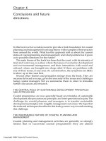
Evidence of intercontinental pollutant transport can be seen in a NASA satellite
photograph of a dust plume traveling from North Africa to the Caribbean, Central
and South America (Figure 8.1). Other photographs are available from NASA on
the World Wide Web.

T

HE

D

ATA

Transcontinental movement of air pollution is a serious issue because it threatens
the ability of nations to achieve their own air quality objectives. Among those
concerns are chronic health impacts and attainment of the national ambient air quality
standards. Recent studies have indicated that transcontinental movement of criteria
and toxic air contaminants, particularly from developing nations to the United States,
is serious and threatens the progress made in attaining our air quality goals.
Among the recent reported findings are:
• Mercury emitted by power plants and factories in China, Korea, and other
parts of Asia travels to the United States and settles into the nation’s lakes
and streams.
•EPA estimates that 40% of the mercury in the air in the United States
comes from overseas.

• Aerial- and ground-based sensors have detected the chemical fingerprints
of air pollutants floating across the Pacific and Atlantic oceans.
•Particulate matter and dust from Africa’s Sahara Desert blows west across
the Atlantic Ocean, which raises particulate levels above federal health
standards in Miami and other Southern cities.

FIGURE 8.1

A NASA satellite photograph of a dust plume traveling from North Africa to
the Caribbean, Central and South America.

7099_book.fm Page 212 Friday, July 14, 2006 3:13 PM
© 2007 by Taylor & Francis Group, LLC

Global Concerns

213

• Ozone and visibility reducing aerosols from factories, power plants, and
fires in Asia and Mexico impact pristine spots, such as California’s
Sequoia National Park and Texas’s Big Bend National Park.
• Los Angeles may get as much as 50 parts per billion of the ozone it
monitors in the summer from overseas. According to researchers from
NOAA, air pollution wafting into the United States accounts for 30% of
the nation's overall ozone problem.
By the year 2020, “imported air” pollution will be the primary factor degrading
visibility in our national parks. U.S. law requires the restoration of natural visibility
in places such as Arizona’s Glen Canyon National Recreation Area. But haze caused
by Asian dust storms sometimes obscures the landscape in the parks. The haze could
make it difficult, if not impossible, to reach federal visibility goals, and it impacts

people’s health due to the ultrafine particle size of the haze.

C

ONCLUSIONS

Intergovernmental cooperation in reducing air pollutants at their source is no longer
restricted to local authorities; it is now needed between nations and continents. If
national long-term air quality goals are to be achieved, it will take the type of
cooperation seen when the problem of stratospheric ozone was addressed, as noted
in the following section.

STRATOSPHERIC OZONE

Probably the most significant success story in global air quality management is the
issue of stratospheric ozone (the ozone hole) and the improvements seen and mea-
sured to date. Human health, and the flora and fauna of a remote location —
Antarctica — were threatened by increased ultraviolet (UV) radiation. To deal with
the threat, reasoned scientific data was applied to a real world problem and a solution
was chosen which worked in an amazingly short time period of less than 20 years. This
issue represents the highest fusion of scientific research, data analysis, and applica-
tion of a global management decision to ameliorate a threat to the environment.

R

ADIATION

P

RIMER

The reason for the concern for stratospheric ozone change lay in the fact that certain
simple molecules absorb incoming sunlight, which contributes to decreases in sur-
face radiation. As seen earlier, there are significant differences between the high
altitude intensity of incoming solar radiation and the intensity measured at sea level.
While it is true that ozone at the earth’s surface is a deleterious material, at high
altitudes it has a beneficial effect by blocking certain wavelengths of harmful solar
radiation as we saw in Figure 5.1 earlier. In Figure 8.2, we see a comparison of
radiation curves over the entire wavelength of incident sunlight, from 0.1 to 100
microns (on a logarithmic scale) and that generated by two surface temperatures:
5800˚ and 245˚K. The curve on the top left is the incident radiation from the sun’s

7099_book.fm Page 213 Friday, July 14, 2006 3:13 PM
© 2007 by Taylor & Francis Group, LLC

214

Principles of Air Quality Management, Second Edition

surface (at 5800˚K) as a function of wavelength. The curve on the top right is the
emission characteristic of the earth’s surface temperature as a function of wavelength.
Incident solar radiation appears in the higher energy (shorter) wavelengths, whereas
that of the earth and its re-radiation is concentrated in the longer or infrared regions.
The overall effect of altitude on radiation absorption is seen in Figure 8.3. All
of the gases from ground level to stratospheric levels contribute to light absorption
(dark areas). A comparison of the radiation absorption at higher altitudes (11 kilo-
meters) to that at the surface indicates the significant absorption due to the depth of
the atmosphere and its constituent gases.
Figure 8.3 illustrates the relative absorptivities of different gases in the top five
bands with a summary in the bottom band. All of the gases in these five bands are

energy-absorbent gases and each has its own characteristic absorption wavelength.

Water is the greatest greenhouse gas of all

because of its strong absorption from
0.8 to over 15 microns, which spans the infrared region. Water, while varying
dramatically, exists in the atmosphere in the range of 0.1 to 7%.
Of significant concern for stratospheric ozone is the third band in Figure 8.3. It
shows the very strong absorption characteristics of oxygen and ozone in the ultra-
violet regions between approximately 0.2 and 0.3 microns. Ozone is primarily
responsible for this absorption. The absorption characteristics of oxygen, while lower

FIGURE 8.2

Radiation emission and absorption curves.
5800°K
245°K
Ground
level
11 km
Black body
curves
0.1 1 2 3 5 10 15 20 30 50 1001.50.2 0.3 0.50.15
(a)
(b)
(c)
0
20
40
60

80
100
0
20
40
60
80
100
Wavelength (microns)
Absorption % Intensity (normalized)

7099_book.fm Page 214 Friday, July 14, 2006 3:13 PM
© 2007 by Taylor & Francis Group, LLC

Global Concerns

215

than ozone, is significant due to its roughly 21% concentration in the atmosphere.
(It is interesting to note that the 6% greater density and oxygen partial pressure of
the atmosphere at the 1,400 foot [below sea] level of the Dead Sea filters out nearly
all of the incident UV radiation such that its beach is a health spa for people with
skin diseases.)
Stratospheric ozone, therefore, serves as a protective layer for the surface of the
earth, since it is known that ultraviolet radiation may have harmful effects not only
on human health, such as skin cancer, but potentially on the phytoplankton in the
earth’s oceans as well.

S

TRATOSPHERIC

O

ZONE

F

ORMATION

The ozone in the upper atmosphere was assumed to be in a steady state condition.
Equations 8.1 through 8.3 indicate the general chemical reactions occurring in the
upper atmosphere.
O

2

+ h

ν



→

2O* (8.1)
O* + O

2

→

O

3

(8.2)
O

3

+ h

ν



→

O

2

+ O* (8.3)
These gases are normally in a natural equilibrium, absorbing ultraviolet radiation
to form ozone and then reforming oxygen with absorption of additional ultraviolet
radiation. The formation and equilibrium concentrations found in various parts of

FIGURE 8.3

Molecule-specific absorption curves.
0.1 0.2 0.3 0.4 0.6 0.8 1 1.5 2 3 4
5 6 8 10 20 30
0
100
100
100
100
CH
4
N
2
O
O
2
and O
3
CO
2
H
2
O
To ta l
Wavelength (microns)
A
b
sorption %

7099_book.fm Page 215 Friday, July 14, 2006 3:13 PM
© 2007 by Taylor & Francis Group, LLC

216

Principles of Air Quality Management, Second Edition

the earth’s atmosphere vary according to latitude, wind velocity, sunspot activity,
and temperature.

E

ARLY

O

BSERVATIONS

The above reactions were not of concern until measured observations indicated a
disturbance of the ozone–oxygen equilibrium over the Antarctic in the 1980s. It
appeared that certain man-made chemicals had a correlation with decreases of the
stratospheric ozone column during October (the Southern Hemisphere’s springtime).
The theory was that anthropogenic emissions of chlorine containing compounds,
including certain gases, chlorofluorocarbons (CFCs), contributed to the perturbation
of the stratospheric ozone equilibrium. Lab studies indicated they had a part in
scavenging the ozone radicals, which depressed the overall formation rate. The CFCs
and related bromine containing compounds were used as refrigerants, solvents, and
fire-extinguishing agents, as well as industrial foam blowing agents.

T

HE

R

ESPONSE

Regulations were implemented which phased out these CFCs in the United States
by 1996. Other nations agreed to phase out the use of CFCs by the year 2000.
Because the diffusion rate of CFCs into the stratosphere is not instantaneous and
there are latitudinal variations in concentration, there was a suggested lag time of
20 to 30 years for the maximum effect of CFCs to the depletion of ozone in the
stratosphere.

O

THER

S

OURCES



AND

V

ARIATIONS

Natural sources of chlorine such as volcanoes were thought to have a significant
impact quite apart from the impact of CFCs in terms of ozone-depletion potential.
Scientists estimate that volcanoes annually dump 12 million tons of hydrochloric
acid into the atmosphere, but only a portion reaches the stratosphere. The 1976
eruption of Mount St. Augustine in Alaska emitted more than 175,000 tons of
chlorine compounds into the stratosphere. Some scientists recall that the 1982
eruption of El Chicon in Mexico thinned the ozone column by 20% as the chlorine-
containing volcanic cloud mixed with the lower portions of the ozone layer.
There were historical disputes as to whether the ozone column changes noted
in the last 15 to 20 years were truly a result of anthropogenic emissions. For instance,
the amount of ozone depends directly on the flux of ultraviolet light from the sun,
which varies with the 11-year solar cycle. There are shorter cyclic periods in solar
output, which will also change stratospheric ozone concentrations. Increases in
sunspot activity, therefore, could be expected to and do indeed contribute to higher
ozone levels in the stratosphere. Satellite data show variations between 0.25 and
0.65% in the stratospheric ozone content every 13.5 days. These variations corre-
spond to changes in ultraviolet emission from the sun, thus verifying that there are
shorter time periods of solar output variability, which also contribute to ozone
variations.

7099_book.fm Page 216 Friday, July 14, 2006 3:13 PM
© 2007 by Taylor & Francis Group, LLC

Global Concerns

217

L

AB

S

TUDIES

The reactions that were found to occur in the laboratory and appeared to show
correlations with ozone depletion in October in the Antarctic are summarized in
Equations 8.4 through 8.6:
CF

2

Cl

2

+ h

ν



→

Cl* + CF

2

Cl* (8.4)
Cl* + O

3



→

ClO + O

2

(8.5)
ClO + O*

→

Cl* + O

2

(8.6)
These lab studies indicated that CFCs slowly migrate to the upper atmosphere
and absorb incident radiation to generate a free radical chlorine atom plus free radical
CFC fragments. In the next step, the free radical chlorine attacks ozone molecules
to yield chlorine monoxide (ClO) and molecular oxygen. The chlorine monoxide
further reacts by scavenging atomic oxygen (free radicals) to yield, once again, the
free radical chlorine atom plus oxygen.
The overall effect, therefore, is for the chlorine free radical to destroy the ozone
as well as oxygen free radicals, which disrupts the normal equilibrium state. This
reaction was held to be responsible for diminishment of ozone concentrations in the

stratosphere. The reason CFCs were found to be important is that they are virtually
nonreactive in the lower atmosphere and slowly diffuse to the stratosphere, where
ultimately they are exposed to high altitude ultraviolet radiation. That ultraviolet
radiation is sufficient to split the molecule, yielding the free radical chlorine atoms.
Laboratory studies indicate that the ozone destruction effectiveness of a chlorine
free radical is between 10,000 and 100,000 oxygen free radicals before it is ultimately
removed from the process by reactions with hydrogen-containing molecules to yield
HCl.

A

NTARCTIC

S

TUDIES

The effect on stratospheric ozone was originally noticed as a short-term phenomenon
in the extreme Southern Hemisphere in early spring rather than a continuous deple-
tion process. Some salient facts on the characteristics of the atmosphere over Ant-
arctica are helpful in the attempt to understand these phenomena.
First, the air over Antarctica is isolated from the rest of the global circulation
patterns during the winter. The patterns are the result of the lack of air disturbances
in the higher southern latitudes due to fewer continental land masses in that hemi-
sphere. This leads to the formation of an isolated polar vortex in which the local
atmosphere is cut off from other air currents. Also significant is the 10 to 20˚K
colder temperatures over Antarctica than over the Arctic. This condition causes
stratospheric ice clouds, which are not seen to the same extent over the northern
high latitudes.

7099_book.fm Page 217 Friday, July 14, 2006 3:13 PM
© 2007 by Taylor & Francis Group, LLC

218

Principles of Air Quality Management, Second Edition

The key appears to be the sudden release of reactive chlorine at the end of the
Antarctic winter (September/October). Nitrogen dioxide reacts in the gas phase with
chlorine monoxide to yield chlorine mononitrate (ClONO

2

). This compound can
convert other chlorine species into chlorine gas, which readily dissociates into
chlorine free radicals. Chlorine mononitrate, when condensed, reacts rapidly with
heterogeneous materials on the surface of an ice particle but not in the gas phase.
Thus, at the very cold air temperatures above Antarctica, virtually nothing happens
during the winter months, except to convert chlorine mononitrate into a solid form
on an ice particle surface. With the first appearance of sunlight in the Southern
Hemisphere springtime, chlorine free radicals are readily formed to enter into reac-
tions with ozone, causing a drop in ozone concentrations during those early spring-
time weeks.
This sequence, coupled with the breakdown of the polar vortex and heating of
the atmosphere in the springtime, causes mixing and dilution of the polar vortex
gases with ozone-containing atmospheric parcels from the Southern Hemisphere to
reestablish the ozone layer over the Antarctic. It has been observed that the tremen-
dous gradients in concentration of ClO and chlorine mononitrate appear to shift by
as much as 5˚

in latitude from one day to the next. This illustrates the importance
of the disturbances of the polar vortex in determining the chemical compositions of
the Antarctic air.
With respect to the Northern Hemisphere, these effects are not seen due to the
warmer temperatures, better atmospheric mixing and lack of available ice particles
to create the sudden loss of stratospheric ozone.

UV D

ATA



AND

O

THER

I

MPACTS

One of the major concerns for potential stratospheric ozone depletion was that UV
radiation would increase. During the period when CFC concentrations in the strato-
sphere were increasing, the ground level UV radiation was monitored.
From these monitored data, it has been found that ultraviolet radiation over the
United States decreased. Figure 8.4 shows the measurements of

decreasing

UV
radiation of as much as 7%. In fact, it was found that ultraviolet radiation over the
United States



decreased during the whole monitoring period. This was a clue that
there were more parameters involved than just ozone concentrations.
The sites in Figure 8.4 illustrate the natural variation in UV radiation to be found
at various locations representative of different latitudes and elevations. Tallahassee
(FL) and Oakland (CA) are at sea level, Minneapolis (MN) is at 255 meters above
sea level, and El Paso (TX) is at 1194 meters. El Paso and Tallahassee are at about
the same latitude (approx. 31˚ north). Oakland is at about 38˚ and Minneapolis is
at about 45˚



north latitude. General trends can be seen in this monitored data. From
Figure 8.4 it appears that the higher the



elevation (El Paso versus Tallahassee), even
at about the same latitude, the higher the UV radiation. Also, the higher the latitude
(all sites), the

lower the incident UV radiation. Location, thus, appears to be the
most significant factor in UV radiation dose.

7099_book.fm Page 218 Friday, July 14, 2006 3:13 PM
© 2007 by Taylor & Francis Group, LLC

Global Concerns

219

Other natural influences that were proposed as factors in explaining these vari-
ations included sunspot activity, atmospheric turbidity, humidity, and cloud cover.
In other studies, National Oceanic and Atmospheric Administration scientists indi-
cated that in the mid latitudes of the Northern Hemisphere, rural ultraviolet radiation
declined between 5% and 18% during the 20th century.
At the same time, the

Journal of Physical Research

used NASA data to dem-
onstrate that global stratospheric ozone levels have increased in recent years at an
average rate of approximately 0.28% per year. Thus, measurements of ozone con-
centrations in the Antarctic were not giving a clear picture of global ozone trends.
Likewise, average effects and measurements for different locations yield significantly
different patterns, or patterns with no statistical significance.

A

LTERNATIVES

With the phase out of CFCs, the challenge has been one of finding substitutes that
could be used for refrigeration and air conditioning. Alternative gaseous chemicals,
some of which are water-based systems, replaced uses of CFCs and other chlorine
containing organics for solvents and foam blowing agents. Substitute refrigerant
gases — HFCs (hydrofluorocarbons) — were the chosen candidates since they have
a zero ozone-depleting potential.
The net result of these U.S. and international actions has been measurable
increases in the ozone column over the last four years over the Antarctic — the most
heavily impacted area.

FIGURE 8.4

U.S. ground level UV radiation, 1974 to 1985.
100
50
150
200
250
74
76 78 80 82 85
Mpls: 255 m; 45°N
Talla, FL: 2 m; 31°N
Oakland: 2 m; 38°N
El Paso: 1194 m; 31°N
Year
UV−RB counts

7099_book.fm Page 219 Friday, July 14, 2006 3:13 PM
© 2007 by Taylor & Francis Group, LLC

220

Principles of Air Quality Management, Second Edition

ACID DEPOSITION

All rainfall is acidic. Pure water has a neutral pH of 7.0 and is the universal solvent.
Consequently it will dissolve all of the gases next to its surface. Thus, raindrops
forming from condensation nuclei will have some dissolved nitrogen, dissolved
oxygen, and all of the gases noted in Chapter 1, including carbon dioxide.
With the exception of ammonia, hydrogen, and the noble gases, atmospheric
gases all have an acidic property. That is, when they are dissolved in pure water,
they will lower the pH into the acid region (pH less than 7). Pollutant gases, such
as sulfur dioxide and chlorine, will also form acids when dissolved in pure water
by reaction with water molecules.

W

ATER

P

LUS

A

IR

One of the major considerations when discussing the effect of gases dissolved in

water is the chemistry of the droplet itself. When there is a dissolution of a gas,
such as carbon dioxide, in water we find not only the dissolved gas, carbonic acid
(H

2

CO

3

), but also an equilibrium between the dissolved gas and its ionized form.
One bicarbonate ion and a free proton are generated from CO

2

. Protons give water
its acidic characteristics. The solution pH in this case is 5.6, in the acid range.
Equation 8.7 (dissolution), therefore, gives rise to Equation 8.8 (dissociation):
H

2

O + CO

2



→

H

2

CO

3

(8.7)
H

2

CO

3



→

H

+

+ HCO

3
-

(pH 5.6) (8.8)
Where other gases (such as ammonia) are present, other reactions are possible
in the aqueous phase. If the acid protons are neutralized by an alkali (Equation 8.9),
the bicarbonate will react further to yield a second proton and a carbonate ion:
HCO

-
3

+ NH

4

OH

→

NH

4
+

+ CO

=
3

+ H
2
O (8.9)

On the other hand, if more protons are added, the equation shifts back to give
more carbonic acid, which will be free to liberate gaseous CO
2
. The overall effect
is a buffering action that acts to keep the pH from changing drastically.
WATER PLUS SOILS
Probably the most significant element of the debate on acid deposition is the influence
of acidic water once it reaches ground level. (This does not take into account acid
fogs, which are a different end product and may have health effects of their own.)
Once rainwater reaches soil, the key element in that new matrix is the relative
percentage of minerals in that soil. In particular, the relative abundance of calcium,
magnesium, and aluminum ions in the soil largely determine the pH of the water
contained therein.
7099_book.fm Page 220 Friday, July 14, 2006 3:13 PM
© 2007 by Taylor & Francis Group, LLC
Global Concerns 221
Alkaline earth minerals (calcium and magnesium) act as basic compounds to
present another buffering action to any acid elements in deposited rain. Thus, an
effect such as Equation 8.10 may be seen:
CaCO
3
+ 2H
+
→ Ca
++
+ H
2
CO
3
(8.10)

In this case, the hydrogen ions are neutralized by calcium carbonate (a typical
component of many soils and rock formations) to yield the calcium ion plus carbonic
acid dissolved in the water. So, the relative abundance of a number of minerals in
the soil has a large effect on pH. The effects of mineral content, as well as humus
and organic acids from plant decay, will reduce soil water pH to between 4.5 and 5.5.
One would expect, therefore, that the more granitic the soil and the fewer
dissolved alkali minerals present, the more likely it is that precipitation pH values
will be unbuffered and more likely to show acid water levels in the pH 4.5–5.5
range. Greater concentrations of alkaline ions in the soil will, therefore, significantly
buffer or neutralize acid components originating in rain.
ACID RAIN STUDIES
Concerns exist for receptor areas downwind of major anthropogenic sources of acidic
gases, such as sulfur dioxide. A number of studies have been performed in the last
few decades reviewing the entire field of anthropogenic acid gas emissions and
receptors such as lakes and streams in North America.
A statistical analyses of early studies (1964 through 1977) on acid deposition
indicated, among other things, that:
1. The annual pH of precipitation showed no long-term significant change
over the period.
2. A linear regression of the data indicated no statistically significant trends
in H
+
deposition.
3. There has been a decrease in SO
4
=
but an increase in NO
3
-
over the same

time period.
Over 80 sites were studied for the follow-up period (1979-1984) for pH, H
+
strength, ion concentrations and precipitation in the northern United States. Table 8.1
summarizes the median concentrations at three of those sites representing a range
of receptor locations with differing upwind air pollution source strengths. From this
study it appeared that the pH and calcium concentrations are directly related —
when the pH is high, the calcium ion strength is high and vice versa. No obvious
correlation appeared between pH and either sulfate, nitrate or ammonium ions.
A different study (1986) made the following conclusions: (1) The eastern half
of the United States experienced ion concentrations of SO
4
and NO
3
that are greater
by a factor of 5 than those levels found in remote parts of the world, and (2) data
on the chemistry of precipitation before 1955 should not be used for trend analysis,
7099_book.fm Page 221 Friday, July 14, 2006 3:13 PM
© 2007 by Taylor & Francis Group, LLC
222 Principles of Air Quality Management, Second Edition
primarily due to the difficulties in establishing a correlation with present methods
of measurement and those used previously.
Other investigators indicated that a pH of 5.6 may not be a reasonable reference
value for unpolluted precipitation pH. Some have questioned the validity of using
pH 5.6 as the background reference due to naturally occurring acids. Likewise, the
times when the rain was collected varied in pH because of the scavenging efficiencies
of rainfall and the times between storms. pH values of rainfall between 4.5 and 5.6
may be due to those natural variabilities alone.
THE NAPAP FINDINGS
The ten-year, $500 million National Acid Precipitation Assessment Program

(NAPAP) was completed in 1990 and then extended under the Clean Air Act Amend-
ments. NAPAP found some significant but similar trends and effects as seen above.
NAPAP employed 700 of the world’s top aquatic, soil, air, and atmospheric scientists
in an exhaustive study on the effect of acid rain on receptor areas as a result of
anthropogenic emissions.
As a part of the NAPAP program, EPA scientists performed an exhaustive study
of correlations between acid precipitation and acidity levels in various receptor
waters. Table 8.2 summarizes the results of that study for two areas that were
suspected of experiencing the highest impact due to high sulfur dioxide emissions.
These two sites were the northeastern United States and the southern Blue Ridge
province in the Appalachian mountain region.
Of the five factors that were investigated for their correlations to surface water
acid neutralizing capacity, acid rain had virtually no correlation in either location.
The highest correlation factor was found to be with the receptor soil’s chemistry
followed by weaker correlations to depth to bedrock (alluvial materials) and geology
(strata). Land usage had only a weak correlation in the northeast and no correlation
in the southern Blue Ridge area. Acid rain had no correlation in either case.
Other evaluations performed during the NAPAP study indicated that Ohio, which
had the highest acid gas emissions in the entire United States, had virtually no acidic
lakes or streams. On the other hand, Florida, which had one of the lowest levels of
TABLE 8.1
Median Variable Ionic Concentration (mg/L)
1979-84 of Atmospheric Deposition Program
(NADP) sites
Ion
Lamberton,
Minnesota
N. Atlantic Lab,
Massachusetts
Kane,

Pennsylvania
pH 6.00 4.67 4.27
SO
4
2–
1.88 1.54 3.48
NO
3
–
1.74 0.73 2.08
NH
4
+
0.81 0.08 0.28
Ca
2+
0.49 0.13 0.16
7099_book.fm Page 222 Friday, July 14, 2006 3:13 PM
© 2007 by Taylor & Francis Group, LLC
Global Concerns 223
acid deposition, had the highest percentage of acidic lakes in the nation at 20%.
These studies indicate that while acid gases such as SO
2
have something to do with
aquatic acidity, they are the least influential factor studied.
As another aspect of the NAPAP study the EPA evaluated pH measurements
taken in lakes over the last 140 years (from historical and secondary data). The
measurements included a comprehensive core sediment analysis of all acidic lakes
(lakes with a pH less than 5.5) in the Adirondack mountains.
This evaluation indicated that not only were 90% of the lakes acidic in 1850,

but the average acidity today is virtually unchanged from preindustrial times. Table
8.3 indicates the changes of pH over time in the Adirondack mountains and in the
Florida acidic lakes. The lakes were grouped into those that had a pH of less than
5.5 and those that had a pH of less than 5.0. The apparent pH change in all cases
was lower by 0.35 pH unit or less. However, it should be noted that the standard
error of the measurement pH was ±0.30 pH units. Except for the most acidic Florida
lakes, there was no statistical change in pH levels measured 140 years ago from
those measured today.
One of the key factors that did occur over this period of time was a dramatic
change in land use patterns and widespread forest clearing. In the mid-19th century,
forests covered many of these areas, and the surface water pH values were relatively
TABLE 8.2
NAPAP Acid Deposition Correlation
Summary: Area Factors
Factor Northeast U.S. S. Blue Ridge
Soil chemistry Fairly strong Fairly strong
Depth to bedrock Moderate Weak
Geology Weak Moderate
Land use Weak None
Acid rain (SO
2
) None None
TABLE 8.3
NAPAP Historical Assessment: Lake Acidity vs. Time
Lake Categories 1850 pH 1986/1988 pH pH Shift Actual Shift*
Adirondack Acid Lakes
pH less than 5.5 4.95 4.78 –0.17 None
pH over 5.0 4.78 4.63 –0.15 None
Florida Acid Lakes
pH less than 5.5 5.11 4.81 –0.30 None

pH over 5.0 5.00 4.65 –0.35 >S.E.
* Standard Error (S.E.) of pH measurement = 0.3 pH units
7099_book.fm Page 223 Friday, July 14, 2006 3:13 PM
© 2007 by Taylor & Francis Group, LLC
224 Principles of Air Quality Management, Second Edition
low (i.e., approximately 5.0). Over the course of approximately 50 to 60 years, the
land was cleared. In each of these cases, the soil chemistry changed due to changes
in the naturally occurring acidic conditions in soil structures. Fires raise soil alka-
linity by replacing acidic forest floor organic compounds with alkaline ash materials.
These alkaline ash materials include the cations calcium, magnesium, and aluminum.
Fires release them from the soil matrix so that they more quickly and easily neutralize
naturally acidic rain. Other soil analyses show that clear cutting of fir forests raises
the pH of the soil from 5.0 to 7.0, and slash-and-burn fires raise it from 4.95 to 7.6.
The National Research Council commented in a paper during the NAPAP study
period that core sediment analyses suggest that acidic lakes were relatively common
in the Adirondack mountains and in New England before the Industrial Revolution.
Woods Lake in that region of New England has a current pH of approximately 4.9.
That is more acidic than the pH 5.6 found in 1915 but practically unchanged from
the 1850s value of pH 5.0. In other words, lakes have been returning to their natural
acidic state from a temporarily more alkaline condition during the period from 1900
to 1940 due to land development by clearing and burning.
CONCLUSIONS
Is there no effect due to acid gas emissions? There are assuredly two effects, one
of which is the addition of gases to the environment, which may have a direct impact
on human health (SO
2
and NO
2
) or indirectly by formation of additional sulfate and
nitrate particulate in condensation nuclei. These have other indirect effects through

particulate matter interactions in the lung. There are also some indications that cloud
layers and fogs tend to concentrate acid gas droplets, which have a detrimental effect
on human health and forests at high elevations where fog and cloud interactions are
more common.
The highest correlation between forest damage and acid deposition from fogs
or clouds is altitude. The decline of red spruce forests at high altitudes has been
found to be correlated with greater percentages of the time when clouds or fogs
encircled these regions. As noted in Chapter 2, direct plant impact in lab studies
using acid mists have been noted due to leeching of nutrients from tree foliage and
the plant crown. Thus, the more concentrated forms of acidic components in fogs
or clouds appear to be better correlated to plant damage.
Natural wash out of soluble soil ions will occur at higher altitudes by gravity
over the course of time. This leads to increasingly poorer nutrient loadings for
vegetation at those elevations. The net effect is increasingly sparse soil with ongoing
reductions in yearly growth, sap flows, and resin. Deficiency in essential nutrients
reduces a plant’s ability to fight disease and to resist insects. The result is an apparent
dying environment.
GLOBAL CLIMATE CHANGE
One of today’s concerns is the suspected impact of anthropogenic air pollutant gases
on global climate. Other concerns are for potential secondary impacts such as rises
7099_book.fm Page 224 Friday, July 14, 2006 3:13 PM
© 2007 by Taylor & Francis Group, LLC
Global Concerns 225
in sea level, flooding of low-lying wetlands, and impacts on agriculture if there is
a proven long-term atmospheric temperature rise or greenhouse effect.
To address this we must first ask, is there a greenhouse effect that causes a
warming of the earth’s surface? The answer is yes, for without a greenhouse effect
due to gases in the atmosphere, the average temperature of the earth’s surface would
be 0˚F. As a consequence of greenhouse gases, the average temperature of the earth’s
surface is approximately 60˚F. Thus, we do experience a global warming impact as

a result of greenhouse gases. The next question is, does the scientific data show an
effect due to anthropogenic gases? Also, what are the greenhouse gases and what
are their sources? Finally, are all of the greenhouse effects “bad”? We will investigate
these items in the following sections.
Most of the effects attributed to anthropogenic gas emissions are based on
computer models attempting to predict temperatures and temperature effects. The
difficulty lies in the fact that weather forecasting computers cannot truly project
what any given location’s temperatures will be within the next week or month, much
less decades in the future. Thus, projections for temperatures in the next century are
even less sure, particularly as a result of air pollutant generated global climate change.
The controversy lies in attempting to verify trends in small temperature changes
(less than 1˚C) while experiencing day to night fluctuations as high as 15˚C. Summer
to winter variations may be as high as 30˚C or more. The other problem lies with
perception, i.e., if it is snowing in Jerusalem and New York City is having its hottest
summer on record, it is hard not to believe that we are facing severe climate changes.
As Steven Schneider of the National Center for Atmospheric Research once said,
“It’s possible that everything in the last 30 years of temperature records is no more
than noise.”
HISTORICAL PERSPECTIVE
Direct measurements of the factors influencing our global climate over time are
restricted to the immediate past few decades. Precise measurements of air temper-
atures and surface sea temperatures have been made for only a few hundred years.
Accurate measurements of certain atmospheric parameters, such as stratospheric
ozone and chlorofluorocarbons concentrations, go back less than 40 years. The first
recorded quantitative measurements of methane in the atmosphere were only made
in 1948.
Consequently, a consideration of historical records is in order since, presumably,
whatever climate changes occurred in the past were without the influence of signif-
icant anthropogenic air emissions. It is known that prior to about 1800 BC, the entire
Middle East experienced a cool, wet climate and forested terrain. By 100 BC, North

Africa was functioning as the grain-growing “breadbasket” for the Roman Empire.
The implication that this geographic area experienced a much cooler, wetter climate
over a time period of 2,000 years is considered valid. Satellite photos that are able
to penetrate the surface sands of North Africa verified that this did occur. These
surface penetrating photos show widespread riverine courses beneath the sands,
which indicate much more extensive runoff and ongoing wetter climates in previous
7099_book.fm Page 225 Friday, July 14, 2006 3:13 PM
© 2007 by Taylor & Francis Group, LLC
226 Principles of Air Quality Management, Second Edition
millennia. As indicated earlier, core sediments from the Dead Sea indicate that
rainfall was abundant in that area until about the fifth century AD.
In the tenth to thirteenth centuries AD, Europe experienced the Medieval Warm
Epoch or “Little Optimum,” in which for several hundred years, the climate was
milder, warmer, and more conducive to civilization in general. Wine grapes were
grown in England, which is not possible today.
At the beginning of the fourteenth century, however, dramatic climate changes
occurred worldwide. The Baltic Sea froze over in the years 1303 and 1306–1307.
Beginning in 1310, cold storms and rises in the Caspian Sea levels were noted
throughout the century. In 1350, in northwest India, the river Mihran disappeared
because of extensive droughts. Monsoons in that era were so weak that droughts led
to widespread starvation. In 1372, Chinese records indicate that sunspot activity
increased to its maximum over a two-century period.
Also in the fourteenth century, the Viking settlement of southern Greenland
provided a well-attested fact of the influence of climate change and its historical
effects. Having been settled in the tenth century during the “Little Optimum,” the
climate in Greenland (hence the name) turned severe with the start of the fourteenth
century. The sites of old farms, now buried in ice, indicate the extent of the settlers’
colonial effort, and the graves of the farmer settlers contain thick masses of plant
roots, which formerly grew under less severe temperatures than those of today. They
are now frozen in soil.

The temperature lowering is further verified by records indicating that marauding
bands of Eskimos, who lived by hunting seals near the edge of the Greenland ice
pack, moved southward attacking and destroying the farming settlements throughout
the fourteenth century. The Eskimos’ southerly movements and records of attacks
indicate that the ice was spreading southward during that era. This was the beginning
of the “Little Ice Age,” which lasted for hundreds of years and was virtually a global
event that reached its maximum between the mid-sixteenth and mid-nineteenth
centuries.
However, from approximately 1850 (at the tail end of the Little Ice Age) and
on into the twentieth century, a warming trend has been experienced. Indeed, certain
glaciers have been found to be retreating in Europe. But glaciers in central Greenland
were found to be growing in the earlier half of the 20th century.
Figure 8.5 is an illustration of the known and estimated temperatures in Great
Britain for approximately the last 10,000 years compared to the average for the first
half of the twentieth century. Approximate departures from the twentieth century
average temperature are shown for summer, winter and annual averages.
Over all of these historical events have been the geogenic factors, such as large
volcanic eruptions, which are proven to dramatically affect climate worldwide for
several years. The 1815 eruption of Mount Tambora in Indonesia, which gave rise
to the “year without summer” in 1816 in America, is an example. The eruption of
Mount Pinatubo in 1991 depressed worldwide temperatures a full degree or more
for two years. Recent studies on the late Roman/early Byzantine Empire indicate
harsh conditions suddenly showing up early in the first decade of the sixth century.
This period corresponds very closely to geologic investigations of Krakatoa, which
appears to have “blown off” in a gigantic explosion about the year 506 AD.
7099_book.fm Page 226 Friday, July 14, 2006 3:13 PM
© 2007 by Taylor & Francis Group, LLC
Global Concerns 227
CURRENT CONCERNS
Concerns are usually expressed for emissions of greenhouse gases, which contribute

to absorption of infrared radiation and potential “global” warming. The greenhouse
gases are seen in Figure 8.6 by their approximate contributions to atmospheric
infrared radiation absorption at current average concentrations.
FIGURE 8.5 Estimated England and Wales temperature for selected periods during the last
10,000 years.
FIGURE 8.6 Greenhouse gas contributions.
Summer
Te mp erature (°C) Departures from 1900–1950 average
Yea rWinter
Pre-boreal Atlantic Sub-boreal
Sub-
Atlantic
Little
optimum
Little
ice age
0
1
2
−1
8300–
7000 BC
6000–
3000 BC
3000–
1000 BC
1000–
500 BC
900–
1200 AD

1500–
1850 AD
Water vapor
Others
NO
x
CO
2
CFCs
CH
4
7099_book.fm Page 227 Friday, July 14, 2006 3:13 PM
© 2007 by Taylor & Francis Group, LLC
228 Principles of Air Quality Management, Second Edition
While there is no small controversy with this issue, it must be remembered that
the major infrared radiation absorbing gas is water. Therefore, discussions that
ignore water vapor do so at the risk of losing a true understanding of the causes of
the greenhouse effect. Most popular estimates of greenhouse gases refer only to
anthropogenic sources of the nonwater vapor gases. This is a serious flaw, since
mankind contributes at most 3% of the nongeogenic CO
2
emissions to the atmosphere
on a global budget basis. Water vapor, at 0.1 to 7% of the total atmosphere, is the
largest single contributor and is not counted in most global climate change scenarios.
Most of the interest to date has focused on anthropogenic emission sources and
the rise in atmospheric carbon dioxide (CO
2
) levels. Figure 8.7 shows a recent
calculation of nongeogenic sources of CO
2

. The graph indicates that of the roughly
800 billion tons of CO
2
accounted for, only 28 billion can be attributed to human
activity worldwide. This does not even consider the geogenic sources of carbon
dioxide. (Mount St. Helens alone averaged 1.8 million tons of CO
2
per year over
the year following the 1980 eruption. Mammoth Mountain, in California, currently
emits between 800 and 1200 metric tons per day of CO
2
or about 0.5 million tons
CO
2
per year on an ongoing basis.)
Even more interesting is the distribution of anthropogenic CO
2
emissions by
location. Figure 8.8 shows the percentage of total man-made CO
2
by global location
calculated for 2000, 2010, and 2020 based on present and estimated global fossil
fuel consumption. This indicates that Asian and Pacific Ocean nations are responsible
for the majority of global CO
2
emissions, ranging from 36% in 2000 to 46% in
2020. The North American (United States and Canada) contribution is calculated to
drop from 28% to 22% by 2020.
Methane is also a greenhouse gas and its concentration is slowly rising. Global
methane budgets, as seen in Table 8.4, indicate that anthropogenic source emissions

FIGURE 8.7 A recent calculation of nongeogenic sources of CO
2
.
100
50
0
150
200
250
300
350
Oceans Vegetation Anthropogenic Soil microbes
223 216
28
331
Billions of tons/year of CO
2
7099_book.fm Page 228 Friday, July 14, 2006 3:13 PM
© 2007 by Taylor & Francis Group, LLC
Global Concerns 229
of methane are approximately 12% of the total, with over half coming from swamps,
marshes, lakes, and rice paddies. Thus the anthropogenic contribution is only a small
player in the methane scenario. There is also a gradient of methane as a function of
latitude on the earth’s surface, as indicated in Figure 8.9, which shows higher
FIGURE 8.8 Percentage of total man-made CO
2
by global location based on present and
estimated global fossil fuel consumption.
Central &
South

America 5%
Asia &
Oceania 41%
Africa 3%
Europe 26%
North
America 25%
Worldwide CO
2
emissions - 2010 AD
Central & South
America 5%
Asia &
Oceania 46%
Africa 3%
Europe 24%
North
America 22%
Worldwide CO
2
emissions - 2020 AD
Worldwide CO
2
emissions - 2000 AD
Central &
South
America 3%
Asia &
Oceania 36%
Africa 3%

Europe 30%
North
America 28%
7099_book.fm Page 229 Friday, July 14, 2006 3:13 PM
© 2007 by Taylor & Francis Group, LLC
230 Principles of Air Quality Management, Second Edition
concentrations of methane measured in the Northern Hemisphere decreasing to lower
concentrations in the Southern Hemisphere. This indicates that methane emissions
are associated primarily with land masses in the Northern Hemisphere.
Not considered are the enormous quantities of geogenic methane locked in
methane hydrates (“methane ices”) on the continental shelves of every major land
mass worldwide. Seepage of geogenic methane may be the dark horse of greenhouse
gases due to the lack of investigation of its emission rate to the atmosphere.
TABLE 8.4
Global Methane Emissions
Source Tons/Year* %
Swamps, lakes, and marshes 146.6 28.8
Rice paddies 142 28
Animals 72 14
Anthropogenic 62 12
Jungles and forests 60 12
Biomass burning (all) 25 5
* Millions
Source: Dr. Don Blake, Ph.D. Dissertation, UC Irv-
ine, 1984.
FIGURE 8.9 Global atmospheric methane distribution versus latitude.
60 60 30 30 0
1.40
1.50
1.60

1.70
ppmv
N Equator S
CH
4
March–May, 1983
7099_book.fm Page 230 Friday, July 14, 2006 3:13 PM
© 2007 by Taylor & Francis Group, LLC
Global Concerns 231
Nitrous oxide (N
2
O) has strong absorption in the infrared radiation band. How-
ever, as seen earlier, N
2
O is the primary NO
x
species given off “by nature.” Indeed,
N
2
O is ubiquitous in the atmosphere and occurs at concentrations of approximately
330 ppb worldwide.
The biggest single problem is that we have essentially no control over the
majority of the emissions of carbon dioxide and no control whatsoever over water
vapor, nitrous oxide, and methane. Thus, our approaches on a global basis must take
these facts into account in any air quality management strategies. Some researchers
have indicated that high altitude clouds or jet aircraft condensation trails are respon-
sible for more of the greenhouse effect than even claimed by the IPCC in 2001.
MEASUREMENTS
Direct measurements are best for attempting to make projections based upon short-
term fluctuations in emissions. For instance, the eruption of Mount Pinatubo in June

1991 cooled the earth’s average surface temperatures by 1–2˚F, which overwhelmed
projections based upon the anthropogenic gases in the atmosphere. Thus, short-term
natural phenomena may cause significant variations that cannot be accounted for in
climate models.
Most of the recent concern for carbon dioxide has been generated by reviewing
CO
2
concentration data over the last 45 years. Typical of these measurements are
those at the Mauna Loa observatory in Hawaii. In Figure 8.10, the atmospheric CO
2
levels at this site since 1958 are plotted. There has been an upward concentration
slope over that period. Attempts at correlations between gas concentrations and
measured average temperatures are more difficult however.
The difficulty in justifying human activities as the source of the change arises
from the fact that observations of temperatures at the earth’s surface do not track
the same rises in CO
2
concentrations. In Figure 8.11 are the temperatures over
FIGURE 8.10 The atmospheric CO
2
levels at the Mauna Loa observatory in Hawaii.
1950 1960 1970 1980 1990 2000 2010
100
50
0
150
200
250
300
350

400
450
5
00
Mauna Loa observatory
Year of measurement
ppm CO
2
7099_book.fm Page 231 Friday, July 14, 2006 3:13 PM
© 2007 by Taylor & Francis Group, LLC
232 Principles of Air Quality Management, Second Edition
130 years in the Northern and Southern Hemispheres, which indicate that the major-
ity of the temperature increase (approximately 0.6˚C to 0.7˚C) occurred prior to
1940. This indicates little correlation of temperature increase in the Northern Hemi-
sphere with the rises in CO
2
noted in Hawaii. Closer inspection of the temperatures
indicates greater variability from year to year than in average trends. Both hemi-
spheres have noted increases over this period. Other problems, of course, are that
even with the best temperature records, the numbers are “fuzzy” by plus or minus
several tenths of a degree.
On a regional basis, Figure 8.12 shows the observed temperatures for approxi-
mately the last 100 years in the continental United States. There has been virtually
no change in average temperatures for the past century when corrected for the urban
heat island effect, as noted earlier.
When one is looking at a shorter time frame, the uncertainty becomes greater.
By taking smaller increments of time, greater fluctuations are seen and pattern
recognition becomes even more difficult. While the Northern Hemisphere had a
slight temperature increase over the last 50 years (which corresponds to the greatest
FIGURE 8.11 Observations of temperature variation from the mean in the (a) Northern and

(b) Southern Hemispheres.
0.4
0.2
−0.2
−0.4
−0.6
0.0
(a)
C°C°
0.4
0.2
−0.2
−0.4
−0.6
0.0
(b)
1870 1890 1910 1930 1950 1990 1970
Yea r
7099_book.fm Page 232 Friday, July 14, 2006 3:13 PM
© 2007 by Taylor & Francis Group, LLC
Global Concerns 233
increases of anthropogenic gas emissions, such as CO
2
), the United States experi-
enced a slight cooling trend. Of course, the year-to-year variability is much greater
than the calculated variation of temperatures over a mean value.
Other trends in maximum daily and minimum nighttime temperatures in the
contiguous United States over the last 100 years indicate that the maximum daily
temperatures increased up until about 1935 and since then have been decreasing. At
the same time, the minimum temperature has been rising. Thus, if a short period

trend analysis conclusion was drawn, it would be that both the daytime high tem-
peratures and nighttime low temperatures were approaching an equilibrium value
and the overall climate was becoming more moderate.
Apart from temperatures, a look at the changes in sea level on a global basis
yields a different pattern. If global warming is truly occurring, a clear pattern of
rising sea levels would be expected at all locations worldwide. Figure 8.13 is an
illustration of changes in worldwide sea levels between 1960 and 1979 around the
world. What has been observed is that the sea level is rising in some locations and
falling in others. Indeed, at some locations in close proximity, such as southern West
Africa, both sea level rises and falls have been observed. It is therefore impossible
to say that any overall sea level rises have in truth occurred.
Changes in sunspot activity have been alluded to with respect to potential climate
change on a historical basis. The sun’s brightness, a measure of its radiation intensity,
affects global temperatures. Likewise, changes in the magnetic field flux of the sun
could impact the earth’s atmosphere and therefore the global heat balance. Indeed,
these may be the events resulting in natural climatic variability.
As noted earlier, the measured changes in air temperature do not match the
emission rates of man-made greenhouse gases. However, it appears that the pattern
of temperature change does match (correlation coefficient of 0.95) the pattern of
changes in the sun’s solar activity for over the last 125 years. Figure 8.14 is a
comparison of solar activity and average global temperatures from 1860 to 1985.
When solar activity increased in the first half of the twentieth century, global
FIGURE 8.12 Annual average temperature for the contiguous United States from 1895 to
1990.
1895 1905 1915 1925 1935 1945 1955 1965 1975 1985
50.0
51.0
52.0
53.0
54.0

55.0
12.7
12.4
12.1
11.8
11.5
11.2
10.9
10.6
10.3
10.0
Yea r
Te mp erature (°F)
Te mp erature (°C)
7099_book.fm Page 233 Friday, July 14, 2006 3:13 PM
© 2007 by Taylor & Francis Group, LLC