Ship Hydrostatics and Stability 2010 Part 13 pot
Bạn đang xem bản rút gọn của tài liệu. Xem và tải ngay bản đầy đủ của tài liệu tại đây (1.78 MB, 26 trang )
Computer methods 305
Figure
13.10
shows that a surface can be described by a net of isoparametric
curves. One procedure for generating a surface can begin by defining a fam-
ily of plane curves, for example ship stations, with the help of Bezier curves,
non-rational or rational
B
-splines,
or NURBS, with the parameter
u.
Taking
then the points u = 0 on all curves, we can fit them a spline of the same kind
as that used for the first curves. Proceeding in the same manner for the points
u = 0.1,
. . .
,
u = 1, we obtain a net of curves. Plane curves can be prop-
erly described by breaking them into spline segments and imposing continuity
conditions at the junction points. Similarly, surfaces can be broken into patches
with continuity conditions at their borders. The expressions that define the
patches can be direct extensions of plane curves equations such as those described
in the preceding sections. For example, a tensor product Bezier patch is
defined by
ij
-J
i|m
(u)J
J>
H,
u=[0,
1],
™
= [0, 1]
i=0
j=0
where the control points,
B^
define a control polyhedron, and
Ji^
m
(u)
and
Jj,n
(
w
)
are
tne
basis
functions we met in the section on Bezier curves. There are
more possibilities and they are described in detail in the literature on geometric
modelling.
13.2.7 Ruled surfaces
A particular case is that in which corresponding points on two space curves are
joined by straight-line segments. For example, in Figure
13.11
we consider three
of the
constant-it;
curves shown in Figure
13.10.
Then, we draw a straight line
from a u = i point on the curve w
=
0.6 to the
u
= i point on the curve
w = 0.7, for i — 0, 0.1,
,
1. The surface patch bounded by the w
=
0.6 and
the w
=
0.7 curves is a ruled surface. A second
ruled-surface
patch is shown
between the curves w —
0.7
and w = 0.8. Ruled surfaces are characterized by
the fact that it is possible to lay on them straight-line segments.
13.2.8 Surface curvatures
In Figure
13.12,
let N be the normal vector to the surface at the point P, and V,
one of the tangent vectors of the surface at the same point P. The two vectors, N
and V, define a plane,
TTI,
normal to the surface. The intersection of the plane
TTI
with the given surface is a planar curve, say C. The curvature of C at the point
P is the normal curvature of C at the point P in the direction of V. We
note it by
k
n
.
A theorem due to
Euler
states that there is a direction, defined by
the tangent vector
V
m
i
n
,
for which the normal curvature,
k
m
-
m
,
is minimal, and
306 Ship
Hydrostatics
and Stability
u=0
"W=0.8
w=0.7
w=0.6
Figure
13.11
Two ruled surfaces
another
direction,
defined
by the
tangent vector
V
max
,
for
which
the
normal
curvature,
/c
max
,
is
maximal. Moreover,
the
directions
V
m
i
n
and
V
max
are
perpendicular. The curvatures
k
m
i
n
and
/c
max
are called principal curvatures.
For example, in Figure
13.12
the planes
TTI
and
7T
2
are perpendicular one to the
other and their intersections with the ellipsoidal surface yields curves that have
the principal curvatures at the point from which starts the normal vector N. The
two curves are shown in Figure
13.13.
Figure
13.12
Normal curvatures
Computer methods 307
Figure 13.13 Principal curvatures
The product of the principal curvatures is known as Gaussian curvature:
•**•
~
"'min
'
"'max
\ij.l
and the mean of the principal curvatures is known as mean curvature:
~r
(13.20)
In Naval Architecture, curvatures are used for checking the fairness of surfaces.
A surface with zero Gaussian curvature is developable. By this term we under-
stand a surface that can be unrolled on a plane surface without stretching. In
practical terms, if a patch of the hull surface is developable, that patch can
be manufactured by rolling a plate without stretching it. Thus, a developable
surface is produced by a simpler and cheaper process than a non-developable
surface that requires pressing or forging. A necessary condition for a surface
to be developable is for it to be a ruled surface. Cylindrical surfaces are devel-
opable and so are cone surfaces. The sphere is not developable and this causes
problems in mapping the earth surface. Readers interested in a rigorous
theory of surface curvatures can refer to Davies and Samuels
(1996)
and Marsh
(1999).
The literature on splines and surface modelling is very rich. To the books
already cited we would like to add Rogers and Adams (1990), Piegl (1991),
Hoschek and Lasser
(1993),
Farm
(1999),
Mortenson
(1997)
and Piegl and Tiller
(1997).
308 Ship Hydrostatics and Stability
13.3
Hull
modelling
13.3.1 Mathematical ship lines
De Heere and
Bakker
(
1970)
cite Chapman
(FredrikHenrikaf
Chapman, Swedish
Vice-
Admiral
and Naval Architect,
1721-1808)
as having described ship lines
as early as 1760 by
parabolae
of the form
y = 1 -
x
n
and sections by
In 1915, David Watson
Taylor
(American Rear Admiral,
1864-1940)
published a
work in which he used 5-th degree polynomials to describe ship forms. Names of
later pioneers are Weinblum, Benson and Kerwin. More details on the history of
mathematical ship lines can be found in De Heere and Bakker (1970), Saunders
(1972, Chapter 49) and
Nowacki
et
al
(1995). Kuo (1971) describes the state
of the art at the beginning of the 70s. Present-day Naval Architectural computer
programmes use mainly
B-splines
and NURBS.
13.3.2 Fairing
In Subsection 1.4.3, we defined the problem of fairing. A major object of the
developers of mathematical ship lines was to obtain fair curves. Digital comput-
ers enabled a practical approach. Some early methods are briefly described in
Kuo
(1971),
Section 9.3. A programme used for many years by the Danish Ship
Research Institute is due to
Kantorowitz
(1967a,b). Calkins et al (1989) use
one of the first techniques proposed for fairing, namely differences. Their idea
is to plot the
1st
and the 2nd differences of offsets. In addition, their software
allows for the rotation of views and thus greatly facilitates the detection of
unfair
segments.
As mentioned in Subsections 13.2.2 and 13.2.8, plots of the curvature of ship
lines can help fairing. Surface-modelling programmes like
MultiSurf
and
Sur-
faceWorks (see next section) allow to do this in an interactive way. More about cur-
vature and
fairing
can be read in Wagner, Luo and Stelson
(
1
995),
Tuohy,
Latorre
and Munchmeyer (1996),
Pigounakis,
Sapidis and
Kaklis
(1996) and
Farouki
(1998). Rabien (1996) gives some features of the
Euklid
fairing programme.
13.3.3
Modelling with MultiSurf and
SurfaceWorks
In this section, we are going to describe a few steps of the hull-modelling process
performed with the help of MultiSurf and SurfaceWorks, two products of Aero-
Hydro. We like these surface modellers for their excellent visual interface, the
Computer methods 309
possibilities of defining and capturing many relationships between the various
elements of a design, and the wide range of useful point, curve and surface types.
A recent possibility is that of connecting
SurfaceWorks
to SolidWorks.
The programmes described in this section are based on a concept developed
by John Letcher; he called it relational geometry (see Letcher, Shook and Shep-
herd, 1995 and
Mortenson,
1997, Chapter 12). The idea is to establish a hierarchy
of dependencies between the elements that are successively created when defin-
ing a surface or a hull surface composed of several surfaces. To model a surface
one has to define a set of control, or supporting curves. To define a supporting
curve, the user has to enter a number of supporting points; they are the con-
trol points of the various kinds of curves. Points can be entered giving their
absolute coordinates, or the coordinate-differences from given, absolute points.
Moreover, it is possible to define points constrained to stay on given curves or
surfaces. When the position of a supporting point or curve is changed, any depen-
dent points, curves or surfaces are automatically updated. Relational geometry
considerably simplifies the problems of intersections between surfaces and the
modification of lines.
Both
MultiSurf
and SurfaceWorks use a system of coordinates with the origin
in the forward perpendicular, the
x-axis
positive towards aft, the
y-axis
positive
towards starboard, and the
z-axis
positive upwards. When opening a new model
file, a dialogue box allows the user to define an axis or plane of symmetry, and
the units. For a ship the plane of symmetry is y =
0.
We begin by
'creating'
a set of points that define a desired curve, for example
a station. Thus, in MultiSurf, a first point,
pOl,
is created with the help of the
dialogue box shown in Figure 13.14. The last line is highlighted; it contains
locked
N<ime
= pQ1
User
data
=
Layer = 0
Weight = 0.000
Color = 14
Visibility
= 1
Figure
13.14
MultiSurf,
the dialogue box for defining an absolute
three-dimensional point
310
Ship
Hydrostatics and
Stability
Figure 13.15
MultiSurf,
points that define a control curve, in this case
a transverse section
the coordinates of the point, x = 17.250, y = 0.000, z = 3.000. There is a
quick way of defining a set of points, such as shown in Figure 13.15. In this
example all the points are situated along a station; they have in common the
value x = 17.250 m.
To
'create'
the curve defined by the points in Figure 13.15 the user has to
select the points and specify the curve kind. A Bcurve (this is the MultiSurf
terminology for
B-splines)
uses the support points as a control polygon (see
Subsection 13.2.4), while a
Ccurve
(MultiSurf terminology for cubic splines)
passes through all support points. Figure 13.16 shows the Bcurve defined by
YZ
X
Figure
13.16
MultiSurf, a curve that defines a transverse section
Computer methods 311
\\\
Figure
13.17
MultiSurf,
a surface defined by control curves such as those
in Figure 13.16
the points in Figure
13.15.
The display also shows the point in which the curve
parameter has the value 0, and the positive direction of this parameter.
Several curves, such as the one shown in Figure
13.16,
can be used as support
of a surface. To
'create'
a surface the user selects a set of curves and then,
through pull-down menus, the user choses the surface kind. An example of
surface is shown in Figure
13.17.
Any point on this surface is defined by the two
parameters u and
v.
The display shows the origin of the parameters, the direction
in which the parameter values increase, and a normal vector.
To exemplify a few additional features, we use this time screens of the Sur-
faceWorks
package. In Figure
13.18
we see a set of four points along a station.
The window in the lower, left corner of Figure
13.18
contains a list of these
points. Figure 13.19 shows the
B-spline
that uses the points in Figure
13.18
as
control points. At full scale it is possible to see that the curve passes only through
the first and the last point, but very close to the others. The display shows again
the origin and the positive sense of the curve parameter.
Figure
13.19
is an
axonometric
view of the curve. Figure 13.20 is an ortho-
graphic view normal to the
x-axis.
In Figure
13.21,
we see the same station
and below it a plot of its curvature. In this case we have a simple third-degree
B-spline; the plot of its curvature is smooth. In other cases the curve we are
interested in can be a polyline composed of several curves. Then, the curva-
ture plot can help in fairing the composed curve. Usually, it is not possible
to define a single surface that fits the whole hull of a ship. Then, it is neces-
sary to define several surfaces that can be joined together along common edges.
A surface is defined by a set of supporting curves, for example, the bow profile,
some transverse curves, etc.
Figure 13.22 The wireframe view of a powerboat
Figure
13.22
shows a wireframe view of a powerboat. The hull surface is
composed of the following surfaces: bow round, bulwark, bulwark round, hull,
keel forward, keel aft, and transom.
The software enables the user to view the hull from any angle, for example
as in Figure
13.23.
Other views can be used to check the appearance and the
fairing of the hull. The rendered view may be very helpful; we do not show an
example because it is not interesting in black and white.
Three plots of surface curvature are possible: normal, mean or Gaussian.
We have chosen the plot of normal curvature shown in Figure 13.24. The
•z
Figure 13.23 Rotating the wireframe view of a powerboat
Ship Hydrostatics and Stability
®
Ship Lines:
powerboat-3:3
Figure 13.26 The lines of a powerboat
13.4
Calculations without and with the computer
Before the era of computers, the Naval Architect prepared a documentation that
was later used for calculating the data of possible loading cases. The documen-
tation included:
• hydrostatic curves;
• cross-curves of stability;
• capacity tables that contained the filled volumes and centres of gravity of
holds and tanks, and the moments of inertia of the free surfaces of tanks.
For a given load case, the Naval Architect, or the ship Master, performed the
weight calculations that yielded the displacement and the coordinates of the
centre of gravity. The data for holds and tanks were based on the tables of
capacity. The next step was to find the draught, the trim and the height KM by
interpolating over the hydrostatic curves. Finally, the curve of static stability was
calculated and drawn after interpolating over the cross-curves of stability. It is in
this way that stability booklets were prepared; they contained the calculations
and the curves of stability for several pre-planned loadings. The same method
was employed by the ship Master for checking if it is possible to transport some
unusual cargo.
The above procedure is still followed in many cases, with the difference that
the basic documentation is calculated and plotted with the help of digital com-
puters, and the weight and GZ calculations are carried out with the aid of hand
calculators, possibly with the help of an electronic spreadsheet. However, since
the introduction of personal computers and the development of Naval Architec-
tural software for such computers, it is possible to proceed in a more efficient
way. Thus, it is sufficient to store in the computer a description of the hull and
Computer methods 317
of its subdivision into holds and tanks. The model can be completed with a
description of the sail area necessary for calculating the wind arm. Then, the
user can define a loading case by entering for each hold or tank a measure of
its filling, for example the filling height, and the specific gravity of the cargo.
The computer programme calculates almost instantly the parameters of the float-
ing conditions and the characteristics of stability, and it does so without rough
approximations and interpolations. For example, in a manual, straightforward
trim calculation one has to use the moment to change trim,
MCT,
read from
the hydrostatic curves. Hydrostatic curves are usually calculated for the ship on
even keel; therefore, using the MCT value read in them means to assume that
this value remains constant within the trim range. Computer calculations, on
the other hand, do not need this assumption. The floating condition is found by
successive iterations that stop when the conditions of equilibrium are met with
a given tolerance.
The ship data stored in the computer constitute a ship model; it can be orga-
nized as a data base. In this sense, Biran and Kantorowitz (1986) and
Biran,
Kantorowitz and Yanai (1987) describe the use of relational data bases. John-
son, Glinos, Anderson et
al
(1990),
Carnduf
and Gray
(1992)
and Reich (1994)
discuss more types of data bases. Many modern ships are provided with board
computers that contain the data of the ship and a dedicated computer programme.
Moreover, the computer can be connected to sensors that supply on line the tank
and hold filling heights.
13.4.1 Hydrostatic
calculations
Some hydrostatic calculations are straightforward in the sense that we can per-
form them in a single iteration. For example, if we want to calculate hydrostatic
curves we must perform integrations for a draught
TO,
then for a draught
T\,
and
so on. Chapter 4 shows how to carry out such calculations. Other calculations
can be carried out only by iterations. For example, let us assume that we want
to calculate the righting arm of a given ship, for a given displacement volume,
VQ,
and the heel angle fa. We do not know the draught, TO, corresponding to the
given parameters. We must start with an initial guess,
Ti
n
i
t
,
draw the waterline,
WQ
LQ
, corresponding to this draught and the heel angle
0^,
and calculate the
actual displacement volume. If the guess
Tj
n
it
was not based on previous calcu-
lations, almost certainly we shall find a displacement volume
Vi
^
VQ.
If the
deviation is larger than an acceptable value, e, we must try another
waterplane,
WiLi,
parallel
to the
initial guess waterline,
WQ£O-
This time
we
proceed
in a
more
'educated'
manner. Readers familiar with the Newton-Raphson procedure
may readily understand why we use the derivative of the displacement volume
with respect to the draught, that is the waterplane area,
Ayy.
We calculate a
draught correction
318 Ship Hydrostatics and
Stability
and we start again with a corrected draught
Ti
-
T^
+
ST
We continue so until the stopping condition
|V
0
-V
N
|<6
is
met.
A much more difficult, but frequent problem is that of finding the floating
condition of a ship for a given loading. The input is composed of the displacement
volume and the coordinates of the centre of gravity. The output is the triple of
parameters that define the floating condition, that is the draught, the heel and
the trim. To solve the problem we can think of a Newton-like procedure in
three variables. Such a procedure implies the calculation of a Jacobian whose
elements are nine partial
derivatives.
Not less difficult is the problem of finding
the floating condition of a damaged ship, provided the ship can still float. The
Naval Architect has to find the draught, trim and heel for which the conditions
described in Section
11.3
are met. In physical terms, the Naval Architect must
find the ship position in which the water level in the flooded compartments is the
same as that of the surrounding water and the centres of buoyancy and gravity
lie on a common vertical. Some details of the above problems can be found
in
Soding
(1978). The calculations of hydrostatic data from surface patches is
discussed by Rabien (1985).
Many ingenious methods for solving the above problems have been devised;
by elegant procedures they ensured satisfactory precision in reasonable calcu-
lating times. The methods based on mechanical computers are particularly inter-
esting. Details can be found in older books. For example, an original publication
of a method for calculating lever arms at large heel angles is due to
Leparmen-
tier
(1899).
Other methods for calculating cross-curves of stability are described
by Rondeleux
(1911),
Dankwardt
(1957), Attwood and Pengelly (1960),
Krap-
pinger (1960),
Semyonov-Tyan-Shansky
(no year given), De Heere and
Bakker
(1970),
Hervieu
(1985),
Rawson and Tupper
(1996).
Methods of flooding calcu-
lations are explained, for example, in Semyonov-Tyan-Shansky (no year given)
and De Heere and Bakker (1970).
As mentioned, the first publication about a computer programme for Naval
Architectural calculations is that of Kantorowitz (1958); it contains also an anal-
ysis of calculation errors. The first computer programmes worked in the batch
mode; an input had to be submitted to the computer, the computer produced an
output. For many years the input was contained in a set of punched cards, later it
could be written on a file. An example of such a programme is ARCHIMEDES
written at the University of Hannover (see Poulsen, 1980). The input consists of
several sequences of numbers. One sequence defines the calculations to be per-
formed, a second sequence describes the hull surface, a third sequence defines
the subdivision into compartments and tanks, a fourth the longitudinal distribu-
tion of masses, a fifth defines run parameters such as the draught, trim, the wave
characteristics, and the identifiers of the compartments to be considered flooded.
Computer methods 319
0
Specific Weight
j
64.0224
Zc.g.
Sink
Trim (deg)
Heel
(deg}
0
0
[
QIC
jj
Cancel I
.Vv^'-' r——•;";;>-»-<i
t
Figure 13.27 The
MultiSurf
dialogue box for entering the input for
hydrostatic calculations
The programme ARCHIMEDES could be run for hydrostatic calculations,
capacity calculations (compartment and tank volumes, centres of gravity, and free
surfaces), cross-curves of stability, damage stability, and longitudinal bending.
Many examples in this book were obtained with the ARCHIMEDES programme.
A newer version of the software, ARCHIMEDES II, is described by
Soding
nd
Tongue
(1989).
Recent programmes have a graphic interface that enables the user to build and
change interactively the ship model, to define run parameters and run calcula-
tions. The output consists of tables and graphs.
Hydrostatic calculations can be performed in MultiSurf or SurfaceWorks after
obtaining the offsets (see Figure
13.25).
Figure
13.27
shows the dialogue box
in which the user has to input the height of the centre of gravity, under
Z.c.g,
the draught, under Sink, and the trim and the heel. A rich output is produced;
Figure 13.28 shows only a fragment. A disadvantage of this implementation
is that each
draught-trim-KG
combination requires a separate run. Aerohydro
supplies another programme, Hydro, that enables a more convenient operation
and yields also graphs. So do several packages marketed by other companies.
13.5 Simulations
The term simulation is frequently used in modern technical literature. The word
derives from the Latin 'simulare', which means to imitate, pretend, counter-
feit. In our context, by simulation we understand computer runs that yield an
320 Ship Hydrostatics and Stability
34
stations,
6036 points
Inputs
Sink
4.00
Trim, deg. 0.00
Heel, deg.
0.00
Dimensions
¥.L.
Length
18.50
fl.L.
Fwd.
X
-1.80
¥.L.
Aft X
16.70
Displacement
Volume 681.8
Displ't.
43653.1
LCB
(%
w.l.)
89.1
Uaterplane
¥.F.
Area 12.52
LCF
(%
TJ.I.)
11-5
Wetted
Surface
¥etd.Area
613.29
Ctr.
tf.S. Z
-3.07
Lateral Plane
L.P.
Area 132.81
Ctr. L.P.
Z
-3.43
Initial
Stability
Trans.
GM
3.89
Spec.
¥t.
Z
e.g.
W.L.
Beam
Draft
Ctr.Buoy. X
Ctr.Buoy. Y
Ctr.Buoy. 2
Ctr.Flotn. X
Ctr.
U.S.
X
Ctr. L.P.
X
Trans.RHPD
64,02
-3.00
5.11
6.00
14.68
-0.00
-3.14
0.33
15.30
13.23
2963.2
Figure
13.28
A fragment of the output of hydrostatic calculations carried
out in
MultiSurf
approximation of the behaviour of a real-life system we are interested in. The
steps involved in this activity are described below:
1.
The building of a physical model that describes the most important features
of the real-life system.
2. The translation of the physical model into a mathematical model. Many math-
ematical models are composed of ordinary differential equations that describe
the evolution of physical quantities as functions of time.
3.
The translation of the mathematical model into a computer programme.
4. The running of the computer programme and the output of results.
For several good reasons the physical model cannot describe all features of the
real-life system. First, we may not be aware of some details of the phenomenon
under study. Next, to use manageable mathematics we must accept simplifying
assumptions. Last but not least, we must keep the computation time within
reasonabe limits and to achieve this we may be forced to accept more simplifying
assumptions.
It follows that computer
simulations
do not exactly reproduce the behaviour
of real-life systems; they only
'simulate'
part of that behaviour. Better results
Computer methods 321
can be certainly obtained by experiments, especially at full scale. It is easy to
imagine that full-scale experiments on ships may be very expensive so that they
cannot be carried out frequently. Dangerous experiments that can lead to ship loss
may not be possible at all. Such tests can be performed only on reduced-scale
models. Still, basin tests too are expensive and their extent is usually limited
by the available budget. Simulations may replace dangerous experiments, basin
tests can be completed by simulations. Then, part of the possible cases can be
simulated, part tested on basin models. The basin tests can be used to correct or
validate the computer model.
It is possible to measure the motions of a ship model in a test basin equipped
with a wave maker. Then, the motions are recorded as functions of time. It is
also possible to simulate ship motions as functions of time, that is to simu-
late in the time domain. However, such measurements or simulations in the
time domain have limitations. As explained in Chapter 12, the sea surface
is a random process; therefore, ship motions are also random processes. To
simulate a given spectrum in the basin or in a computer programme, it is
necessary to draw a number of random phases. The resulting motions do not
describe all possible situations, but are only an example of such possibilities. We
say that we obtain a realization of the random process. Moreover, for practical
reasons, the duration of a basin test is limited. Then, the time span may not
be sufficient for the worst event to happen. Although we may afford simulation
times longer than basin tests, they still may be insufficient for obtaining the worst
events.
More results can be obtained by calculating motions as functions of frequency,
that is calculating in the frequency domain. Programmes that perform such
cal-
culaitons are available both through universities and on the market. The software
calculates the added masses and damping coefficients, for a series of frequen-
cies, by using potential theory and certain simplifying assumptions. Next, the
software calculates the response amplitude operators, RAOs, of various motions
or events. For a wave frequency component, and given ship heading and speed,
the programme calculates the frequency of encounter and transforms the spectra
from functions of wave frequency to functions of the frequency of encounter.
Response spectra are obtained as products of the spectra of encounter and RAOs.
Statistics can be extracted from the spectra, for instance root mean square,
shortly RMS values of the
motions.
Taking into consideration the motion of the sea surface, the heave and the pitch,
the programme yields the motion of a deck point relative to the sea surface and
calculates the probability of having waves on deck. Other events whose proba-
bility can be calculated are slamming and propeller racing, while the motions,
velocities and accelerations of given ship points are obtained as combinations
of motions in the various degrees of freedom. An example of ship motions
simulated in the time domain can be found in
Elsimillawy
and Miller
(1986).
Examples of studies of capsizing in the time domain are in
Gawthrop,
Kountzeris
and Roberts (1988) and Kat and Paulling (1989). An example of simulation in
frequency domain is given by Kim, Chou and Tien (1980).
322 Ship
Hydrostatics
and
Stability
13.5.1
A simple example of roll simulation
Subsection 9.3.2 shows how to implement in MATLAB a Mathieu equation and
simulate the roll motion produced by parametric excitation. More complicated
models can be simulated in a similar manner by writing the governing equations
as systems of first-order differential equations and calling an integration routine.
The more complex the system becomes, the more difficult it is to proceed in this
way. The programmer must write more lines and arrange them in the order in
which information must be passed from one programme line to another. Software
packages have been written to make simulation easier. The common feature of
the various packages is that the programmer does not have to care about the order
in which information must be passed. Also, routines and functions frequently
used in simulations are available in libraries from which the user can readily
call them. The programmer has only to describe the various relationships, the
software will detail the equations and arrange them in the required order. In this
section we give one very simple example of the capabilities of modern simulation
software. As we give in the book examples in MATLAB, it is natural to use here
the related simulation package, SIMULINK. Let us consider the following roll
equation
Az
2
0
+
gkGZ
=
M
H
(13.21)
where A is the displacement mass,
i,
the mass radius of inertia, GZ, the righting
arm, and MH, a heeling moment. We rewrite Eq.
(13.21)
as
rr
(13.22)
In this example we neglect added mass and damping, but use a non-linear func-
tion for GZ and can accept a variety of heeling moments. To represent this
equation in SIMULINK we draw the block diagram shown in Figure
13.29
by
putting in blocks taken from the libraries of the software and connecting them
by lines that define the relationships between blocks. At the beginning we put
two blocks representing heeling moments,
MH.
For the wind moment we use
a step function. Initially the moment is zero, at a given moment it jumps to a
prescribed value that remains constant in continuation. For the wave moment we
use a sine function, but it is not difficult to input a sum of sines.
The next block to the right is a switch; it is used to select one of the heel-
ing moments,
M
H
.
The block called Heeling arm performs the division of
the heeling moment by the displacement value supplied by the block called
displacement. Follows a summation point. At this point the value gGZ is
subtracted from the heeling arm. The output of the summation block is
MH
*
Displacement
Wind moment
Product
1 Integrator
Integrator!
Wave moment
Gain = g Righting arm
Conversion
roll
Figure 13.29 Simulating roll in SIMULINK
324 Ship Hydrostatics and Stability
Continuing to the right, we find a block that multiplies by
l/i
2
the output of the
summation block; the result is
/M
H
We immediately see from Eq. (13.22) that the output of the block called
Product 1 is the roll acceleration,
<j).
This acceleration is the input to an inte-
grator. The symbol
1
5
that marks the integrator block reminds the integration of Laplace transforms.
The output of the integrator is the roll velocity,
0,
in radians per second. The
roll velocity is supplied as input to two output blocks. One block, above at right,
is an
oscilloscope,
shortly
scope,
marked
Phase
plane.
The
other block,
an
integrator marked
Integrator
1,
outputs
the
roll angle,
<p.
Following a path to the left, the roll angle becomes the input of a block
called
Righting
arm. This block contains
GZ
values
as
functions
of
(/>.
In
a gain block the GZ value is multiplied by the acceleration of gravity,
g,
and
at the summation point, the product is subtracted from the heeling arm. Fol-
lowing
rightward
paths, the roll angle is supplied directly to the scope Phase
plane,
while converted
to
degrees
is
input
to the
scope
Heel
angle.
The
scope
phas
e p 1 ane displays the roll velocity versus the roll angle. The scope
angle
displays
the
roll
angle versus time.
13.6 Summary
Ship projects require the drawing of lines that cannot be described by simple
mathematical expressions, and also extensive calculations, mainly iterated inte-
grations. Interesting attempts have been made to use mathematical ship lines,
but until the second half of the last century the procedures for drawing and fair-
ing ship lines remained manual. As to calculations, many elegant methods were
devised, not a few of them based on mechanical, analogue computers, such as
planimeters, integrators and
integraphs.
As in other engineering fields, in the
domain of Naval Architecture the advent of digital computers greatly improved
the techniques and made possible important advances. Naval Architects were
among the first engineers to use massive computer programmes.
The development of computer graphics has made possible the use of com-
puters in the design of hull surfaces. In computer graphics, curves are defined
parametrically
where the parameter,
t,
is frequently normalized so as to vary from 0 to
1
.
Computer
methods
325
The central idea in computer graphics is to define curves by piecewise poly-
nomials. In simple words, the interval over which the whole curve should be
defined is subdivided into subintervals, a polynomial is fitted over each subinter-
val
and conditions of continuity are ensured at the junction of any two intervals.
The conditions of continuity include the equality of coordinates at the junction
point and the equality of the first, possibly also the second derivative at that
point. The latter conditions mean continuity of tangent and curvature.
The simplest examples of curves used in computer graphics are the Bezier
curves. The coordinates of a point on a Bezier curve are weighted means of the
coordinates of
n
control points that form a control polygon. The degree of the
polynomial representing the Bezier curve is n —
1.
An extension of the Bezier
curves are the rational Bezier curves; they can describe more curve kinds than
the non-rational Bezier curves.
Moving a control point of a Bezier curve produces a general change of the
whole curve.
B-splines
avoid this disadvantage by using a more complicated
scheme in which the polynomials change between control points. Moving a
control point of a
B-spline
produces only a local change of the curve. A pow-
erful extension of the
B-splines
are the non-uniform rational
B-splines,
shortly
NURBS. Computer programmes for ship graphics use mainly B-splines and
NURBS.
Naval Architectural calculations involve many integrations. The calculations
for hydrostatic curves can be performed straightforward. Other calculations can
be carried out only by iterations, e.g. for finding the cross-curves of stability or
the floating condition of a ship for a given loading, possibly also a given damage.
Systematic and elegant methods were devised for performing the calculations
with acceptable precision, in a reasonable time. Many methods used mechanical,
analogue computers. When digital computers became available it was possible
to write computer programmes that performed the calculations in a faster and
more versatile way. The first programmes worked in the batch mode. The input
was first introduced on punched cards, later on files. The programme was run
and the output printed on paper. Present-day programmes are interactive and
graphic user interfaces facilitate the input and yield a better and pleasant output.
The interface enables the user to build and change interactively the ship model.
This model includes the definitions of the hull surface, of the subdivision into
compartments, holds and tanks, the materials in holds and tanks, and the sail
area required for the calculation of wind arms.
Another use of computer programmes is in the simulation of the behaviour of
ships and other floating structures in waves or after damage. Thus, it is possible
to study situations that would be too dangerous to experiment them on real
ships. Simulations can be carried out in the time domain or in the frequency
domain. In the latter approach, one input is a sea spectrum, the output consists
of spectra of motions and probability of events such as deck wetness, slamming
or propeller racing. Simulations are used also for studying the stability of ships
in the presence of parametric excitation. When the model used in simulation
consists of ordinary differential equations the work can be greatly facilitated by
326 Ship Hydrostatics and Stability
using special simulation software. Then, the user employs a graphical interface
to build the model with blocks dragged from libraries. The software produces
the governing equations and arranges them in the order required for a correct
information flow.
13.7 Examples
Example 13.1 - Cubic Bezier
curve
%BEZIER Produces the position vector of a cubic
%Bezier spline
function P
=
Bezier(BO,
Bl,
B2,
B3)
% Input arguments are the four control points
%
BO,
Bl,
B2,
B3 whose coordinates are given
% in the format [
x;
y
].
Output is the
% position vector P with coordinates given in
% the same
format.
% calculate array of
coefficients,
in fact
% Bernstein polynomials
t = [ 0:
0.02:
1 ] '
;
% parameter
CO
=
(1 -
t).~3;
Cl
=
3*t.*
(1 - t)
.~2;
C2 =
3*t.~2.*
(1 - t)
;
C3 =
t.~3;
C
=
[ CO Cl C2 C3 ]
;
% form control polygon and separate coordinates
B = [ BO Bl B2 B3 ]
;
xB =
B(l,
:)
;
yB =
B(2,
:)
% calculate points of position vector
xP =
C*xB';
yP =
C*yB';
P = [
xP';
yP'
]
13.8 Exercises
Exercise 13.1 - Parametric ellipse
Write the MATLAB commands that plot an ellipse by means of Eq. (13.4).
Exercise 13.2 - Bezier curves
Show that the sum of the coefficients in Eq. (13.9) equals 1 for all t values.
Arscott,
P.M.
(1964).
Periodic Differential Equations -An Introduction to Mathieu, Lame
and Allied Functions. Oxford: Pergamon Press.
ASTM (2001). Guide F1321-92 Standard Guide for Conducting a Stability Test (Light-
weight Survey and Inclining Experiment) to Determine the light Ship Displacement
and Centers of Gravity
of
a Vessel.
http://www astm.org/DATABASE.CART/PAGES/
F1321.htm.
Attwood, E.L. and Pengelly, H.S. (1960). Theoretical Naval Architecture, new edition
expanded by Sims,
A.J.
London: Longmans.
Bieri,
H.P. and Prautzsch, H. (1999). Preface. Computer Aided Geometric Design, 16,
579-81.
Biran, A. and
Breiner,
M. (2002).
MATLAB
6 for Engineers. Harlow, England: Prentice
Hall. Previous edition translated into German as: MATLAB 5 fiir Ingenieure - System-
atische
und
praktische
Einfiihrung
(1999). Bonn:
Addison-Wesley.
Greek translation
1999, Ekdoseis Tziola.
Biran, A. and Kantorowitz, E. (1986). Ship design system integrated around a relational
data base. In
CADMO
86 (G.A.
Keramidas,
and T.K.S.
Murthy,
eds), pp. 85-94,
Berlin:
Springer-Verlag.
Biran,
A.,
Kantorowitz, E. and Yanai, J. (1987). A Relational Data Base for Naval Archi-
tecture. In International Symposium on Advanced Research for Ships and Shipping in
the Nineties,
CETENA's
25th Anniversary, S.
Margherita
Ligure, Italy, 1-3 October.
Birbanescu-Biran, A. (1979). A system's theory approach in Naval Architecture. Inter-
national Shipbuilding Progress, 26, No. 295, March, 55-60.
Birbanescu-Biran, A. (translated
and
extended) (1982). User's Guide
for
the Program Sys-
tem
"Arhimedes
76" for hydrostatic calculations. Technion. See also original, Poulsen
(1980).
Birbanescu-Biran, A. (1985). User's guide for the program
STABILfor
intact stability
of naval vessels, release 2. Haifa: Technion.
Birbanescu-Biran, A. (1988). Classification systems for ship items: a formal approach
and its application. Marine Technology, 15, No.
1,
67-73.
Bjorkman,
A. (1995). On probabilistic damage stability. The Naval Architect, Oct.,
E484-5.
Bonnefille,
R. (1992). Cours
d'Hydraulique
Maritime, 3rd edition. Paris: Masson.
Borisenko,
A.I. and Tarapov, I.E. (1979). Vector and Tensor Analysis with Applications,
translated and edited by
Silverman,
R.A.
New York: Dover Publications.
Bouteloup, J. (1979).
Vagues,
Marees,
CourantsMarins.
Paris: Presses Universitaires de
France.
Bovet, D.M., Johnson, R.E. and Jones, E.L. (1974). Recent Coast Guard research into
vessel stability. Marine Technology, 11, No. 4, 329-39.
Brandl, H. (1981).
Seegangsstabilitat
nach der
Hebelarmbilanz
auf
Schiffen
der Bundes-
wehr-Marine.
Hansa, 118, No. 20, 1497-503.
Burcher, R.K. (1979). The influence of hull shape on transverse stability. In
RINA
Spring
Meetings, paper No. 9.
Calkins,
D.E.,
Theodoracatos, V.E.,
Aguilar,
G.D. and Bryant, D.M. (1989). Small craft
hull form surface definition in a high-level computer graphics design environment.
SNAME
Transactions,
97,
85-113.
Cardo,
A.,
Ceschia,
M.,
Francescutto, A. and Nabergoj, R. (1978).
Stabilita
della
nave
e
movimento
di rollio: caso di momento sbandante non
variabile,
Tecnica Italiana,
No. 1,
1-9.
Bibliography 329
Carnduff,
T.W. and Gray,
W.A.
(1992). Object oriented computing techniques in ship
design. In Computer Applications in the Automation of Shipyard Operation and Ship
Design
IV,
pp. 301-14.
Cartmell,
M.
(1990).
Introduction to Linear, Parametric and Nonlinear
Vibrations.
Lon-
don: Chapman and Hall.
Cesari,
L.
(1971).
Asymptotic Behaviour and Stability Problems in Ordinary Differential
Equations. Berlin:
Springer-Verlag.
Chantrel, J.M.
(1984).
Instabilites
Parametriques
dans
le
Mouvement
des Corps Flottants
- Application
au
cas des
bouees
de
chargement,
These presentee a
"Ecole
Nationale
Superieure
de
Mecanique
pour
1'obtention
du
diplome
de
Docteur-Ingenieur".
Paris:
Editions Technip.
Churchill, R.V. (1958). Operational
Mathematics,
2nd edition. New York: McGraw-Hill
Book Company.
Cleary,
C,
Daidola, J.C. and Reyling, C.J. (1966). Sailing ship intact stability criteria.
Marine
Technology,
33, No. 3, 218-32.
Comstock,
J.P. (ed.) (1967). Principles of Naval Architecture. N.Y.: SNAME.
Costaguta, U.F. (1981). Fondamenti di
Idronautica.
Milano:
Ulrico
Hoepli.
Cunningham, W.J. (1958). Introduction to Nonlinear Analysis. New York: McGraw-Hill
Book Company.
Dahle,
A. and Kjaerland, O. (1980). The capsizing of
M/S
Helland-Hansen. The investi-
gation and recommendations for preventing similar accidents. Norwegian Maritime
Research,
8, No. 3, 2-13.
Dahle, A. and Kjaerland, O. (1980). The capsizing of
M/S
Helland-Hansen. The investi-
gation and recommendations for preventing similar accidents. The Naval Architect,
No. 3, March,
51-70.
Dahle, A.E. and Myrhaug, D.
(1996).
Capsize risk of fishing vessels.
Schiffstechnik/Ship
Technology Research, 43,
164-71.
Dankwardt, E. (ed.) (1957)
Schiffstheorie.
In
Schiffbautechnisches
Handbuch, Vol. I,
Part 1 (W.
Henschke,
ed.).
VEB Verlag Technik Berlin.
Davies, A. and Samuels, P. (1996). An introduction to Computational Geometry for
Curves and Surfaces. Oxford: Clarendon Press.
Deakin,
B. (1991). The development of stability standards for U.K. sailing vessels. The
Naval Architect, Jan., 1-19.
De Casteljau, P. de F. (1999). De Casteljau's autobiaiography: My time at Citroen. Com-
puter Aided Geometric Design, 16, 583-6.
De Heere, R.ES. and
Bakker,
A.R. (1970). Buoyancy and Stability of Ships. London:
George G.
Harrap
& Co.
Den
Hartog,
J.P. (1956). Mechanical Vibrations, 4th edition. New York: McGraw-Hill
Book Company.
Derrett,
D.R., revised by
Barrass,
C.B. (2000). Ship Stability for Masters and Mates, 5th
edition. Oxford:
Butterworth-Heinemann.
Devauchelle, P. (1986). Dynamique du Navire. Paris: Masson.
DIN 81209-1 (1999). Geometrie und
Stabilitdt
von
Schiffen
-
Formelzeichen,
Benennun-
gen,
Definitionen.
Teil
I:
Allgemeines,
Uberwasser-Einrumpfschiffe
(Geometry and
stability of ships - Symbols for formulae, nomenclature,
deffinitions.
Part
1:
General,
surface monohull ships).
Dorf,
R.C. and Bishop, R.H. (2001). Modern Control Systems, 9th edition. Upper Saddle
River, N.J.: Prentice-Hall.