Radio Propagation and Remote Sensing of the Environment - Chapter 10 pptx

© 2005 by CRC Press

275

10

General Problems
of Remote Sensing

The second part of this book is dedicated to the background of remote sensing by
radio methods. The notion of remote sensing of the environment is usually understood
as the determination of characteristics of a medium by devices that are far from the
object being studied. The concept of

environment

includes all objects (both natural
and of anthropogenic origin) that form man’s habitat. These are the natural objects
(soil, vegetation, atmosphere, etc.) around us on Earth, as well as near Earth and in
outer space. These objects also include people themselves and animals. Some ele-
The goal of measurements carried out for remote sensing is to define various
environmental parameters that can be used to obtain a deeper understanding of
natural processes, to improve economic activities through the realization of the
preventive actions necessary to protect the environment, and to discover and monitor
extraordinary natural and anthropogenic situations.
The time and spatial scales of observed characteristics have a very wide range
(from part of a second to centuries for time and from units of meters to units of a
global scale for space). The measurers can be mounted on ground and air platforms,
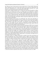
on rockets, and on space craft. Some of these platforms are also shown in Figure 10.1.
Environmental remote sensing assumes the practical absence of disturbance in
the studied medium during measurements. This is achieved by electromagnetic

application or remote sensing acoustic waves. The wide application includes elec-
tromagnetic, microwave, and ultrahigh-frequency waves, all of which interact effec-
tively with natural media. It is supposed that the interaction of electromagnetic waves
with the environment, defined by the electrophysical and geometrical parameters of
the researched objects, is closely connected with the structure, thermal regime,
geophysical characteristics, and other parameters of these objects. Radiowave inter-
the physical background of radio methods for remote sensing of natural media. The
devices for research, as well as the development of processing technology for
experimental data, are created on this basis. In the following chapters, we consider
devices that are used for remote sensing and some methods for processing experi-
mental data. In this chapter, which may be considered as an introduction to remote
sensing, some problems of environmental remote sensing are covered from the
position of radio methods:
•Formulation of the remote sensing problem
• Radiowave bands applied to remote sensing
• Main principles of processing remote sensing experimental data

TF1710_book.fm Page 275 Thursday, September 30, 2004 1:43 PM
action with natural media was described in the first part of this book (Chapters 1 to
9), which was devoted to radio propagation theory in various media. This theory is
ments of the environment are represented schematically in Figure 10.1.
© 2005 by CRC Press

276

Radio Propagation and Remote Sensing of the Environment

10.1 FORMULATION OF MAIN PROBLEM

The main goal of remote sensing is, as was already mentioned, to obtain various

kinds of data about the environment. In this book, we will consider only radiowaves
as the source of such information. Radiowaves are generated from both artificial and
natural sources. The methods applied to artificially generate waves are often called

active

as opposed to

passive

approaches based on using naturally generated waves.
It is necessary to point out that active methods are generally connected with coherent
waves, while incoherent waves are typical for passive methods.
The high frequency power gathered by an antenna at the receiver input is
amplified (often with a frequency decrease due to heterodyning). As a result, one
or several voltages are formatted at the receiver output. Each of them is linearly
related to the field strength entered the measuring system input. Sometimes this
relation has a functional character. Also, the receiving–amplifying part of a device
contributes the complementary noise, the power of which is defined by the receiver
noise temperature (

T

n

). The sources of interference may have another origin, partic-
ularly with regard to extraneous waves at the antenna input. As a rule, interference
is supposed to be additive, although this does not hold in all cases.
The signal from the receiving/amplifying component enters the processing
device, where the required measurement parameters (e.g., amplitude, phase, fre-

quency, delay time) are separated. The processing operation is optionally linear. As

FIGURE 10.1

Schematic representation of the environment.
Environment and platforms with measurers
1. Outer space
2. Ionosphere
3. Atmosphere
4. Earth
OZONE

TF1710_book.fm Page 276 Thursday, September 30, 2004 1:43 PM
© 2005 by CRC Press

General Problems of Remote Sensing

277

a result, the instrument can be mathematically represented as a set of operators (

A

1

,

A

2

, …,

A

i

) converting the characteristics of input strengths

E

in

at the antenna into
the voltages

V

i

at the output. Thus, this relation has a statistical character:
, (10.1

)

where

∆

V

i

is the errors generated by the noises of

i

-th channel of the measuring
instrument or the measuring system.
We will now provide simple examples of the relations of output voltages with
measured quantities of parameters for some instruments. In order to do this, we will
the most frequently used instruments of remote sensing.

10.1.1 R

ADAR

At least two operators, , and , correspond with this instrument. They are
associated with output voltages and , corresponding to two characteristics
of received radiation. One of them is proportional to the time delay between radiated
and received signals and the second one to the received signal power:
(10.2)
where is the power of the

j

-th polarization of the wave in the receiving antenna
input, is the effective area of the receiving antenna at the

j-

th polarization,
is the transmitter power at the

i-

th polarization, is the gain of the transmitting
antenna at the

i

-th polarization,

σ

ij

is the radar cross-polarization section of the target
backward scattering,

R

is the distance from the target to the radar, and

c

(

R

)

is the
radiowave velocity. Signal processing may be more varied. In particular, the oper-
ators of polarization and spectral analyses would be added to the two mentioned
above, which are most commonly used.

10.1.2 S

CATTEROMETER

The scatterometer is a variant of a radar where the power of the received signal is
the only object of measurement. The operator

A

sct

associates the output voltage
with a quantity equal to the ratio of the power at the receiving antenna input
to the power at the transmitting antenna output (

i

and

j

are the corresponding
polarization):

, (10.3)
Vt A E t V
ii i
() ()=
{}
+
in
∆
A
rl
1
A
rl
2
V
rl
1
V
rl
2
Vt A Et t
dR
cR
V
rl rl
R
ij
11
0
2() () ~()

()
,




{}
=
∫
in
ι
222
rl rl
j
ii
tAEt P
PG
ij
() () ~




{}
=
in
rec
rad rad
σ
iij j

A
R
rec
16
24
π
,
P
j
rec
A
j
rec
P
i
rad
G
i
rad
V
ij
sct
P
j
rec
P
i
rad
Vt A Et
P

PR
dl
ij
J
i
sct sct
in
rec
rad
() () ~=
{}
⇒
1
16
22
π
∫∫
() ( ) ()
∫
DlAd
ijij
rad rec
ΩΩΩΩσ
π
,
2

TF1710_book.fm Page 277 Thursday, September 30, 2004 1:43 PM
briefly describe the main points of operators (discussed further in Chapter 11) for
© 2005 by CRC Press

278

Radio Propagation and Remote Sensing of the Environment

where is the transmitting antenna directional coefficient at the

i-

th polarization.
On the right side is the integral with respect to depth

l

and over the solid angle as
a distributed object of our research (e.g., cloud drops, ionospheric electrons, sea-
surface irregularities). Therefore, in the considered case, is the cross section
per volume unit. It is supposed that the target is distributed in some volume; thus,
we have an integral with respect to

l

. It is assumed further that the layer thickness
is much less than the distance to the radar, and the integration over

Ω

is mainly
concentrated within the major lobe of a pencil-beam antenna. This gives us the
opportunity to put distance

R

outside the integral sign. If we deal with a surface
target (sea ripples, for example), it is necessary to assume that
, where is a dimensionless value (cross section per
area unit or backscattering reflectivity). When the backscattering reflectivity is a
constant, Equation (10.3) is quite simplified and, at the matched polarization:
(10.4)

10.1.3 R

ADIO



ALTIMETER

The radio altimeter is also a functionally simplified radar. The main interest here is
the arriving time of the signal; the operator

A

alt

relates output voltage to the
time interval (

τ

) between the radiated and received radio pulses:
, (10.5)
where

h

is the altimeter altitude above a reflecting surface, and

c

(

h

) is the radiowave
velocity depending on altitude.

10.1.4 M

ICROWAVE



RADIOMETER

The operator

A

rm

associates the output voltage with a quantity that is proportional
to the brightness temperature of an object:
. (10.6)
The operators mentioned above will be refined later when we describe specific
techniques for calibration will also be given in Chapter 11. This calibration allows
us to estimate the coefficients of proportionality and permanent biases that are
negligible in Equations (10.2) to (10.6).
D
i
rad
σ
ij
l(, )Ω
σσδ
ij
llR
ij
(, ) ( ) ( )ΩΩ= −
0
σ
ij
0
()Ω
AEt
P
P
A
R
j

j
j
sct
in
rec
rad
rec
() ~
()
.
{}
⇒
σ
π
0
2
0
4
V
alt
Vt A Et t
dh
ch
h
alt alt
in
() () ()
()
=
{}

⇒ =
∫
τ 2
0
Vt A Et P T
ii j
rm
in
rec
rm
() () ~=
{}
⇒


TF1710_book.fm Page 278 Thursday, September 30, 2004 1:43 PM
instruments used for remote sensing (Chapter 11). Information about the primary
© 2005 by CRC Press

General Problems of Remote Sensing

279

10.2 ELECTROMAGNETIC WAVES USED FOR REMOTE
SENSING OF ENVIRONMENT

Remote sensing of the natural environment is realized within a wide range of
of the range has its own merits and demerits; therefore, the most effective approach
is the application of different areas of the electromagnetic spectrum as appropriate.
We consider in this book only part of the radio region: millimetric, centimetric,

decimetric, and, particularly, ultrahigh frequency (UHF). The advantage of using
this spectral part of the region as opposed to the optical or infrared is connected
with the depth of penetration that can be achieved in a medium which allows us to
detect variation in medium parameters related to the depth of the structure. Using
vehicle-borne instruments, radiowaves are absorbed weakly in the atmosphere and
clouds. This creates the conditions for all weather observations of Earth’s surface.
In addition, the application of radio instruments, as opposed to optical ones, does
not require illumination of the area being studied by solar light, which allows us to
carry out investigations regardless of the time of day. Also, some spectral intervals
in this region interact effectively with the ionosphere, atmosphere, and atmospheric
formations, as well as with elements of ground and sea surfaces. This gives us the
opportunity to use them to investigate these media.
The main drawback of using the radio region is the rather low (in comparison
to the optical and infrared regions) spatial resolution, especially by passive sounding
(see Equation (1.120)). Only synthetic aperture radars overcome this difficulty and
achieve spatial resolution comparable with optical and infrared devices (see

FIGURE 10.2

Electromagnetic waves, which can be used for remote sensing of the
environment.
UV OPT
0.28−0.38 µ 0.38−0.78 µ 0.78−3 µ 3−8 µ 8−1000 µ
3·10
−7
3·10
−6
3·10
−5
3·10

−4
3·10
−3
3·10
−2
3·10
−1
10
8
10
9
10
10
10
11
10
12
10
13
10
14
10
15
3
λm
λ cm
fHz
0.1
0.1
0.3 3 30 100

100 10 1
fΓHz
PLSCXK
u
K
a
Kmm
IR

TF1710_book.fm Page 279 Thursday, September 30, 2004 1:43 PM
Chapter 11).
electromagnetic waves — from ultraviolet to radio (see Figure 10.2). Each section
© 2005 by CRC Press

280

Radio Propagation and Remote Sensing of the Environment

Effective application of radiowaves to investigate natural objects depends on the
required spatial resolution and specific peculiarities of radio propagation in the
experimental conditions. The problem of various objects interacting with electro-
In the case of sounding from space through the ionosphere, the lower limit of
the frequency region (

f

min

) is determined by the maximum of the ionospheric plasma
frequency (

f

p

) connected with the maximum of electron concentration

N

max

(see

p

concentration maximum is on the order of 10 MHz. The limitations connected with
wave propagation in the ionosphere are naturally no longer relevant to the use of
airborne instruments; however, they appear again if, for example, we are dealing
The upper frequency border of the sounding region from space is defined by the
atmospheric absorption of electromagnetic waves. The main absorbing components
are water vapor and oxygen. In the radio band, oxygen has a series of absorption
lines at a wavelength of 0.5 cm and a separate line at a wavelength of 0.25 cm.
Water vapor has absorbtion lines corresponding to wavelengths 1.35 and 0.163 cm,
and also a series of absorption lines at waves shorter then 1 mm. As absorption at
frequency 3 ·10

11

Hz is of the order at 10 db this frequency is assumed to be the
upper border frequency region for the radio sensing of Earth from space. Hence, the

electromagnetic region of sounding waves from space is determined by the inequality
.
The transparency windows of the millimetric wave region lie at the wave bands of
One has to take into account when planning experiments the help of both aerospace-
borne instruments and devices mounted on the ground. Meteorology radar, in par-
ticular, is a common example. It is fitted to take into consideration radiowave
scattering and absorption by hydrometeors (clouds, rains, snow).
In underground sounding, an important consideration is the depth of penetration
into the researched layers, and UHF is the band used in this case. A similar band is
Frequencies lying at the transparency windows and at regions of selective atmos-
pheric absorption, depending on the problem being studied, are applied for the study
of the atmosphere and atmospheric formations. The waves of millimetric, centime-
tric, and decimetric bands, depending on the requirements for the sounding depth
and spatial resolution, are also preferable for the study of biological objects.
Remote sensing with radiowave help is based, as indicated earlier, on changes
in the wave characteristic as a result of interaction with the environment. The change
in radiowave characteristics is detected by the receiving systems. The output signals
then allow us to obtain the position, form, and geophysical parameters of natural
formations.
01 10
3
, <<λ cm

TF1710_book.fm Page 280 Thursday, September 30, 2004 1:43 PM
magnetic waves is discussed in Chapters 12 to 15.
Equation (2.31)). It was pointed out in Chapter 2 that the value of f in the electron
with upper ionosphere observations (see Chapter 3).
also applied for ionospheric research for other reasons (see Chapters 3, 13, and 15).
0.2, 0.3, 0.8, and 1.25 cm (Figure 10.3) in the absence of clouds, snow, rain, etc.
© 2005 by CRC Press

General Problems of Remote Sensing

281

Listed below are the main radiowave characteristics determined by remote
sensing:
• Amplitude, intensity, and power flow of the electromagnetic field
•Time of propagation
• Direction of the radiowave propagation
• Phase properties of radiowaves
• Frequency and frequency spectrum of receiving signal
• Polarization characteristics of received signal
• Change of the pulse shape
In order to obtain information about the geometry, physico-chemical properties,
structure, state, and dynamics of a natural formation, we must formulate an inverse
problem to study the change of these values in space and time and use

a priori

information about the investigated object itself and about the characteristics of its
interaction with the electromagnetic field.

10.3 BASIC PRINCIPLES OF EXPERIMENTAL DATA
PROCESSING

The main goal for thematic processing of experimental data obtained through envi-
ronmental remote sensing is to define the characteristics of a medium in space and
time. As a rule, such characteristics are the values related to its physico-chemical
properties, structure, etc. In order to reach this goal, we must solve a wide range of

problems that are referred to as inverse ones from the point of view of causal and
investigatory connections. However, it is an inverse problem in only some cases —

FIGURE 10.3

Microwave absorption due to atmospheric gases: 1, normal humidity (7.0
g/m

3

); 2, humidity (4 g/m

3

).
0
50
100
150
200
250
300
0.01
0.1
1
10
100
1000
1
2

frequency (GHz)

TF1710_book.fm Page 281 Thursday, September 30, 2004 1:43 PM
© 2005 by CRC Press

282

Radio Propagation and Remote Sensing of the Environment

namely, those having a great number of unknown parameters (where the state of an
object is described by some coordinate function); we will discuss those problems
further toward the end of this chapter. The other inverse problems have been given
such labels as problems of classification, factorization, parameter estimation, model
discrimination.

83,84

We have divided these problems into three groups according to
the requirements for remote sensing data processing:
• Classification problems are related to defining the type of object being
observed and its qualitative characteristics (e.g., space observation of land
areas where it is difficult to distinguish forest tracts from open soil or ice
plots from open water).
•Parameterization problems are connected with the numerical estimation
of parameters of studied objects (e.g., not a question of what we see during
a flight above the ocean, but rather determining the surface temperature
of the water or the seawave intensity).
•Inverse problems of remote sensing are associated with the creation of
continuous profile distributions for various parameters of the researched
objects (e.g., height profiles of tropospheric temperature, height profiles

of ionospheric electron concentration).
The problems of classification deal with the selection of object groups having
approximately similar parameters with regard to interaction with electromagnetic
waves and, consequently, as one may expect, comparable physico-chemical and
structural characteristics. One can subdivide a body of mathematics for classification
based on different directions of cluster (grouping close results of multidimensional
measurements) and structure (grouping of spatio-temporary areas with structures of
close multidimensional measurements) analyses, as well as multidimensional scaling
(limitation by magnitude).

84

The classification problem is generally solved by multichannel methods; how-
ever, before turning to them, let us say a few words about some of the possible
single-channel methods. The simplest one is associated with the establishment of
boundaries for the functional quantities of instrument output voltages (parameters
of interaction) within limits, where the investigated objects may be related to a
particular class. The simplest kind of such functionals can be maximum and mini-
mum values, medians, dispersion, correlation coefficients of experimental,

a priori

data, etc. Obviously, the boundaries themselves are established on the basis of

a
priori

information (from theory or previous experimental data often obtained by

in

especially its having multiple modes can be used for classification (Figure 10.4b).
The elements of the textured analyses can be applied in the case of sufficient

a priori

information. These elements may relate to the specific form of signal from defined
elements of the sounding environment and with the contours of two-dimensional
images.
The technique of multidimensional scaling is seldom applied for multichannel
measurements (thresholds are established from

a priori

data similarly to the one-
channel case). More often, in this case, we resort to different methods of cluster

TF1710_book.fm Page 282 Thursday, September 30, 2004 1:43 PM
situ methods) (see Figure 10.4a). The characteristics of the distribution function and
© 2005 by CRC Press

General Problems of Remote Sensing

283

analyses. As a rule, three types of information are taken into consideration: multi-
dimensional data of measurements, data about closeness after processing the exper-
imental materials, and data about classes obtained as a result of experimental and

a

priori

data processing multidimensional data chosen from the train of data obtained
from different measurement channels. The closeness criterion here is defined by the
parameters of discrepancy or similarity for the separated sets (clusters) of the exper-
imental data, such as intercorrelation data in different measurement channels, the
intersection of data, or other similar parameters (e.g., the Euclidean distance between
two similar objects or some other functional closeness).
For classification purposes, the ensemble of experimental points (comparable
according to some feature) is intercepted in the measurement space. This process is
known as

clusterization

. The set boundaries are defined by the expected credibility
value of the obtained results. From this point of view, the intuition of the researcher
plays no small role here. These boundaries may be ascertained in the process of

FIGURE 10.4

(a) Schematic image brightness temperature around Antarctica; (b) histogram
of this temperature. I, sea; II, sea ice; III, continental ice.
300
200
100
13 57 9 1311 15 17 19 21 23 25 27 29 3331 35
Coordinate point number
I
I
I

III
III
II II
II
T
b
T
b
(a)
(b)
120.0
140.0
160.0
180.0
200.0
220.0
240.0
260.0
12
10
8
6
4
2
0
N

TF1710_book.fm Page 283 Thursday, September 30, 2004 1:43 PM
© 2005 by CRC Press

284

Radio Propagation and Remote Sensing of the Environment

establishing the relations of these sets with the elements of the studied environment.
This process, known as

cluster identification

, is usually realized by teaching and is
carried out for unknown objects by measuring various elements of the known
environment and subsequently comparing these measurement results with the out-
come of the cluster processing. The results of theoretical and experimental research
can be also used for the identification. Many standard computer programs are
available for cluster analysis of experimental data. The example of ice field cluster-
ization on the basis of remote sensing at three microwave channels is discussed in
Livingstone et al.

136

The texture methods, as compared to cluster methods, are associated with another
type of classification. If the cluster techniques classify objects by single elements
of the spatial resolution of an instrument, then the texture methods do so according
to the structure of the fields of the observed objects. Continuous fields are usually
considered, but it is also possible to examine noncontinuous fields. The body of
mathematics regarding this area is extensive, it is well algorithmized, and numerous
computer programs are available for texture analyses. Figure 10.5 shows the results
of the texture procedure for the selection of forest tracts.

137,138

Certainly, other more complicated methods of pattern recognition are available,
but the techniques described briefly above have gained the widest application for
remote sensing. It is necessary to point out once more that the need to address these
methods is conditioned by the complicated structure of many natural objects and
the practical impossibility of computing exactly the results of their interaction with
electromagnetic waves. Therefore, these methods do not assume knowledge of the
relations between some parameters of the environment and the characteristics of
their interaction with electromagnetic fields; however, knowledge of interaction

FIGURE 10.5

(a) Application of two classification stages of forest types with a usage texture
parameter; (b) application for classification of a trizonal artificial neural network; (c) image of a
fir forest obtained as a result of processing synthetic aperture radar (SAR) data.
(a) (c)
(b)
6
3
2
1

TF1710_book.fm Page 284 Thursday, September 30, 2004 1:43 PM
© 2005 by CRC Press

General Problems of Remote Sensing

285

models facilitates both the clusterization and identification of separated clusters and

cluster spatial structures.
Before turning to the second group of problems (problems of parameterization),
let us consider briefly the factorial approach to remote sensing problems. This
approach is associated with both the classification and the parameterization of natural
formations. Parameters such as atmospheric humidity, water content and temperature
of clouds, temperature of the sea surface, soil moisture, vegetation biomass, and
factors. The simplest factorial problems (e.g., assessing the influence of a small
number of known causes) are solved, as a rule, by regressive analysis technique.

139

In regressive analyses, we graph the regressive curves reflecting the statistical rela-
tion between numerical values of factors (e.g., soil moisture, biomass of vegetation)
and parameters of the radiowave interaction with the medium being researched, such
as brightness temperature or the scattering cross section. An example of a one-
dimensional linear regression of two variables,

x

and

y

,



is provided in Figure 10.6.
The regressive line is plotted by the experimental points

y

j

based on
the condition
dependence on the subsoil water level) give an example of the regressive line use
in remote sensing. The regressive lines inclination angles may be used in some cases
for the identification (classification) of factors.

FIGURE 10.6

(a) Straight line of regression

y

on

x

and straight line of regression

x

on

y

; (b)
regression for the same field of a correlation, where and are average values of the

variables.
012345678
x
−2
−1
0
1
2
3
4
5
6
7
8
9
10
y
x
y
y
^
− y
x
^
= b’y + a’
y
^
− y
x
^

− x
x
^
− x
x
^
− x
x
^
− x
r
xy
= 0.686
y
^
= bx + a
y
^
− y
y
^
− y
x
^
− x
x
y
ˆ
ybxa=+
()

yy
jj
j
−
()
∑
ˆ
2

TF1710_book.fm Page 285 Thursday, September 30, 2004 1:43 PM
many other characteristics (described in Chapters 12 to 16) can be considered as the
. Figure 15.12 (brightness temperature with regard to
© 2005 by CRC Press

286

Radio Propagation and Remote Sensing of the Environment

To solve more complicated problems related to unknown causes, different vari-
ants of the factorial analyses are applied. In this case, the processing of experimental
data obtained by a large number of measurement channels (more than the number
of expected factors) takes place. These data have to be associated with the terrain
coordinates and have similar spatial resolution. The data are joined in the rectangular
matrix

Y

for the factorial processing. The rows of this matrix determine the mea-
surement channels and columns — the results of measurements along the definite
curve on the terrain. This matrix is called a

matrix of data

. Analysis of this matrix
allows us to obtain information about the primary factors influencing the variation
of experimental data corresponding to defined areas of the studied terrain.
These factors are classified as

common

and

specific

ones by their effect on
experimental data. The specific factors influence only one channel; the common
factors that affect all processed channels are also referred to as

general

. The data
are normalized for the factorial analysis, and matrix

Y

is rearranged into the so-called
standardized matrix

Z

with the elements:
, (10.7)
where is the main signal value in the

i

-th channel, and is the standard deviation
in the same channel.
Factorial analysis is practically reduced to standardized data presentation as a
linear combination of hypothetical variables or factors:
(10.8)
Here, are coefficients (determined during factor analysis) that define the influence
grade of the

j

-th common factor; are factor scores (the numerical value of
influencing characteristics) at the

j

-th sample; and is the common effect of the
unique factors of

i

-th channel. This equality expresses the basic model of factor
analysis. Thus, it is supposed that the matrix of standardized data is defined only
by common factors, and by applying the matrix form of notation we obtain:
. (10.9)

Matrix

A

is the

factor pattern and its elements, , are factorial loadings. Matrix
P represents by itself the matrix of numerical quantities (parameters) of the factors
.
The fundamental theorem of factorial analysis maintains that matrix A is related
to the correlation matrix R, the elements of which are the correlation coefficients
between rows (channels) of standardized matrix Z. In the case of uncorrelated
factors,
, (10.10a)
zyy
ij ij i i
= −()/σ
y
i
σ
i
zapap ap
ij jij i irrj
i
=+ +++
11 2
2
.ζ
a
ij

pp
jrj1

ζ
i
ZAP=
a
ij
p
ij
RAA= '
TF1710_book.fm Page 286 Thursday, September 30, 2004 1:43 PM
© 2005 by CRC Press
General Problems of Remote Sensing 287
where is the transposed matrix of the factorial loads, and
(10.10b)
in the case of correlation of factors. C is the correlative matrix reflecting the relations
between factors.
Matrix C is computed on the basis of a priori information about the physical
connections between factors. Matrix A is defined by solving Equation (10.10a). The
method of main components or the centroidal method is often applied for these
purposes.
Different models of factorial analysis are used depending on the accepted a
priori assumptions. We can separate these models into two groups. For the first
group, we assume that the number of common factors is known. Then, the factor
loads a
ij
and the numerical quantities of the factors p
ij
are determined from Equation

(10.10a). In the process, the summarized dispersion added by the negligible factors
in the general data dispersion of each channel, is minimized.
For models of the second group, we must first determine the number of common
parameters required to provide affinity of experimental and calculated correlation
matrixes. To do so, we use the sequential approach technique, from one to n common
factors. The computation is stopped when the differences between elements of the
experimental and calculated matrix reach the same order as the measurement and
computation errors. It is useful to point out that, in this case, computation of the
common factors is performed by applying Equation (10.10a) where the reduced
matrix R
h
is substituted for the correlation matrix R. Matrix R
h
differs from matrix
R by its diagonal terms, which are called the commonalities in this case. The
commonalities give us an estimation of the contribution of the common factors to
the common data dispersion in the processed segment. The commonalities estimation
is a separate problem of factorial analysis. A rough estimation is sufficient in the
case of a great number of channels; for example, the maximal value of nondiagonal
terms of the chosen row can be used for the diagonal term. The qualitative side of
The first group of factorial analysis models is more appropriate for problems of
parameter estimation; the second group, for classification problems. The factorial
models perform linearization of experimental data on the given segment of process-
ing and estimate the quantity and the intensity of the factors impacting the output
signal change. Factorial analysis is especially useful for the preliminary simultaneous
processing of a great number of channels.
Parameterization problems belong to the main class of remote sensing problems.
They are connected with quantitative estimation of the parameters of the natural
object being studied. It is supposed in the process of problem solving that the model
function relates the instrument displays with the structure and physico-chemical

properties of the objects. This relation depends upon the accuracy of the parameters;
a priori model functions may be refined and modified during specific studies. Some
these functions were addressed in the first part of this book and will be examined
in following chapters with regard to significant objects of the environment. Here,
′
A
RACA= '
TF1710_book.fm Page 287 Thursday, September 30, 2004 1:43 PM
such classification is demonstrated by Figure 10.7.
© 2005 by CRC Press
288 Radio Propagation and Remote Sensing of the Environment
we will consider only some general problems of estimating the parameters of a
function.
Suppose that model functions F
i
connect measured electromagnetic wave param-
eters I
i
of the i-th channel with the studied objects characteristics, x
j
. Then, we can
write the following system for calculating the parameters of the medium:
, (10.11)
including in the consideration the measurement errors, , and the model concep-
tion uncertainties, . Here, i is the measurement channel number, n is the number
of parameters to be determined, and are summarized errors of the
FIGURE 10.7 (A) Three channels have one general factor; (B) three channels have two
general factors; (C) three channels have one common factor (o) and two general factors (a
and b).
I channel

II channel
III channel
I channel
II channel
III channel
I channel
II channel
III channel
(C)
(B)
(A)
Factor o Factor a
Factor a
Factor a Factor a
Factor b
Factor b
IFxx x
immn
ii n i
=+
= ≥
(, , , )
,, , ,
12
12
∆
∆
i
()1
∆

i
()2
∆∆ ∆
ii i
=+
() ( )12
TF1710_book.fm Page 288 Thursday, September 30, 2004 1:43 PM
© 2005 by CRC Press
General Problems of Remote Sensing 289
i-th channel. It is often supposed that the error distribution function is known, even
if only approximately, and it is taken into account in the solution process.
The considered system is not quite an ordinary one solvable by higher algebra
technique. On the one hand, if x
j
and are regarded as unknown values, then the
system is not definite because the number of unknown values is always more than
the number of equations. On the other hand, we can neglect the measurement errors
by assuming them to be equal to zero. In this case, the number of equations is usually
more than the number of unknown parameters and the system becomes contradictory.
The solution of Equation (10.11) is divided into two steps:
140
(1) definition of
unknown parameters using the minimum of data, and (2) definition of unknown
parameters by using redundant data. These two steps are closely connected, and the
processing may be confined by one of them.
By processing using a minimum of data selection from Equation (10.11), then
the number of equations being equal to the number of unknown parameters is n = m,
assuming the errors to be equal to zero. We usually solve the obtained nonlinear (in
the general case) system of equations by applying the iterative procedure. In most
cases, this procedure results in a sufficiently good initial approximation of the

unknown parameters by using the techniques of reassembly and rear-
rangement of equations and by varying the initial conditions and other combinations.
This can be done even in the absence of a priori data regarding the environmental
parameters being studied. After this, it is convenient to linearize Equation (10.11)
by the following expansion:
(10.12)
where distinguishes parameter x
j
from the starting approach, .
The system of linear equations in Equation (10.12) may be solved by changing
by the methods for the solution of redundant equations (see later) on the
assumption that the errors are equal to zero. In this way, we are processing
the linear model by the minimum of data. The problem is then reduced to solution
of the linear equations ( = 0):
∆
i
xx x
n1
0
2
00
,, ,
IFxx x Fxx x
ii n ii n
=+= +(, , , ) ( , , , )
12 1
0
2
00
∆∆∆

i
ij
xx
j
j
n
Fx x i m
jj
+
+=
=
=
∑
∂∂ δ/| ,,, ,
0
1
12
δx
j
x
j
0
δx
j
∆
i
()
∆
i
I

I
aa
aa
x
x
n
n
nnn
n
1
11 1
1
1
.
.

.
.

.
.
=
TF1710_book.fm Page 289 Thursday, September 30, 2004 1:43 PM
© 2005 by CRC Press
290 Radio Propagation and Remote Sensing of the Environment
or
I = AX.
The solution will have the form:
(10.13)
where the matrix is the inverse one. The inverse matrix appears when the matrix

determinant differs from zero; however, if the matrix elements are given approxi-
mately, then the question about the determinant of matrix differing from zero is
irrelevant. This observation relates particularly to cases when a change of coefficients
in the frame of accuracy can change the determinant sign. A system having such a
matrix cannot be solved with sufficient accuracy. The matrix is a stable one when
small changes of basic matrix elements lead to small changes of inverse matrix
elements. If the inverse matrix is unstable, then the basic matrix is an ill-conditioned
one. It is clear that we must choose experimental conditions that will lead to a stable
matrix of the linear equations.
The determinant of the basic matrix must not be too small to provide stability
of the inverse matrix. It is difficult to define precisely the notion of “too small”
because multiplication of the matrix by any quantity changes the determinant but
does not change the inverse matrix stability.
141
Hadamard’s inequality can be used
as a diagnostic criterion for the determinant value estimation:
. (10.14)
Hadamard’s inequality has to be close to equality for inverse matrix stability. Obvi-
ously, the experimental conditions must be chosen in such a way as to give us the
opportunity to obtain the maximum of the matrix M determinant; in particular, it
can be done by choosing data for these channels that lead to value maximization of
the determinant.
The next step of analysis is redundant data processing. The random errors are
assumed to be basic and other ones can be neglected. If the last condition is not
fulfilled, the considered methods give biases. We can select from the two major
groups of methods to obtain estimations by redundant measurements.
83,140
We must
know the distribution function of observed values to apply the first group of methods;
the maximal likelihood and Bayes’ methods are commonly used, and they will be

covered below. The regressive method, the method of minimal squares, and the
method of minimal modules are related to the second group. They allow estimations
close or equal to the maximal likelihood ones on the basis of the formal computing
techniques without knowledge of the distribution function for the observed values.
XAI
1
=
−
A
1−
A
||A ≤
=
=
∑
∏
a
ij
j
n
i
n
2
1
1
TF1710_book.fm Page 290 Thursday, September 30, 2004 1:43 PM
© 2005 by CRC Press
General Problems of Remote Sensing 291
Let us consider the method of maximal likelihood to define the environment
parameters on the basis of measuring data in m channels. In the process, m > n. The

density of joint distribution (f) can be represented in the form:
(10.15)
for the case of independence of individual measurements.
83,140
The function
is the function of likelihood. It is a joint distribution function for the observed
quantities and is regarded as a function of unknown parameters x
i
. The observed
environment parameter quantities obtained by the likelihood function maximum are
referred to as reliable estimations or estimations of maximal likelihood. Maximal
likelihood estimations are distributed by the normal law under very common con-
ditions. They are mutually effective and therefore consistent. The mathematical
expectation of the estimation tends to approach the true value with an increasing
number of measurements.
Taking into consideration the exponential view of the distribution function, the
maximization of the logarithm of the likeliness function usually is used; that is,
(10.16)
The value L can be maximized relative to x by setting the partial derivatives equal
to zero; thus,
(10.17)
The solution of these equations gives us the unknown estimations. We have achieved
processing using the minimum of data, as the number of equations is equal to the
number of the unknowns. Equation (10.17) is reduced to a linear one when the model
functions are linear and the distribution function is normal. The method of the reverse
matrix may be used in this case to solve the equation system.
Estimation by Bayes’ method is based on maximization of a posterior probability
distribution for the investigated parameters which are considered as random values.
The a posteriori probability distribution is:
fI I I x x x fI x x x

mn n
(, ,,,,,,)(,,, , )
12 1 2 1 1 2
……= ffI xx x fI xx x
gI
nm n
m
(,,, , ). ( , , , , )
(
212 12
=
112 1 2
,, , | , , , ) ( | )IIxxxgIx
mnm
=
gIx
m
(|)
LIx gIx fIxx x
mm jn
j
m
(/)ln(/) ln (, ,, , )==
=
∑
12
1

∂
∂

∂
∂
∂
∂
L
x
fI x x x
x
L
m
jn
j
m
m
1
12
1
1
0==
=
∑
ln (, ,, , )
;
xx
fI x x x
x
n
jn
n
j

m
==
=
∑
∂
∂
ln (, ,, , )
.
12
1
0
TF1710_book.fm Page 291 Thursday, September 30, 2004 1:43 PM
© 2005 by CRC Press
292 Radio Propagation and Remote Sensing of the Environment
, (10.18)
where is a posterior distribution of probability (i.e., the density of the
probability distribution for when observations are obtained by this time);
is the mutual density of distribution for and ; is the function
of likelihood; is the a priori density of distribution ; is the a priori
density of distribution for the observation results .
All values of x are supposed to be equally probable if a priori information about
the distribution function is lacking. In this case, Bayes’ estimations coincide with
the maximal likelihood ones. We may expect refinement of the maximal likelihood
method when a priori distribution is known to be due to the additional
information. This refinement takes place for a limited number of channels. The
contribution of the additional information becomes negligibly small as a result of
an unlimited increase in the number of channels, and the maximal likelihood esti-
mations coincide asymptotically with the Bayes’ method ones.
Now, let us to turn to the second group of processing techniques. The first one
we will consider here is the regressive method.

142
We can write down the system of
m equations for n unknown values in the matrix form (m > n)”
.
We know that X = M
–1
I at m = n. We can obtain a good linear estimation for X
when m > n by using a similar formula:
(10.19)
where M is Fisher’s information matrix:
, (10.20)
is the errors dispersion in j-th channel, and . Thus, the
dispersion matrix equals M
–1
.
This estimation minimizes the sum of the squares of the weighted deviations on
the right and left sides of the equations. If the measurements in channels are
uniformly precise and their dispersion is unknown, we can substitute unity for the
dispersion. The estimation, in this case, minimizes not the weighted deviations but
simply the sum of deviations squared. As a result of estimating this parameter, we
obtain:
gxI gIx gI gIxgx gI
01021
(|) (,)/ () (|) ()/ ()==
gxI
0
(|)
x I
gI x
(,)

I x gIx
0
(|)
gx
2
() x gI
1
()
I
gx
2
()
IAX I AX===
×
mmnn
XMY
1
=
−
MFFY F=
′
=
==
∑∑
11
2
1
2
1
σσ

j
jj
j
m
j
jj
j
m
I;
σ
j
2
F
iii in
aa a=
12
,, ,
TF1710_book.fm Page 292 Thursday, September 30, 2004 1:43 PM
© 2005 by CRC Press
General Problems of Remote Sensing 293
, (10.21)
as well as the estimation of dispersion. A similar regressive method is applied for
the solution of the nonlinear equation. The iterative procedure is needed for realiza-
tion of this technique.
The criterion function method
140
is applied to solve the system of equations:
, (10.22)
where I
i

are the measurement results, F
i
are the model functions, and x
j
are parameters
of the model functions being defined. We can substitute the quantities of any param-
eter into these equations. The differences between the mea-
sured quantities and values generated by the model function are referred to as the
discrepancy. Those parameter quantities are assumed to be the system solution that
correspond to the minimum of some objective function for the discrepancies
.
It is necessary to choose the objective function in such a way as to obtain
estimations as close as possible to those of maximum likelihood. In practice, the
most applicable are the objective functions for the discrepancy of the sum of
weighted squares:
(10.23)
where w
i
are weighting coefficients. If the model errors are stochastic and the
accuracy of the measurements is not sufficiently high, then we must assume that the
errors are distributed not by Gaussian law but by Laplace’s law. In this case, we
need to minimize the objective function that is the sum of the discrepancy modules:
(10.24)
If, in practice, the distribution function differs from the one assumed for analysis,
then the estimation obtained will have dispersions larger than the maximal likelihood.
The ratio of this dispersions is referred to as the effectiveness of estimation.
(f
1
, normal; f
2

, Laplace; f
3
, gamma; f
4
, Cauchy) and four minimizing functionals:
σ
21
2
1
= −−
′




−
=
∑
()mn I
jj
j
m
XF
IFxx x i mmn
ii n
==>(, , , ), , , , )
12
12 (
x
j

0
()
∆∆ ∆
12
,, ,
m
()
Φ∆ ∆ ∆
1 2
,, ,
m
()
Φ
112
2
1
= −
()




=
∑
wI Fxx x
ii i n
i
m
,, , ,
Φ

212
1
= −
=
∑
wI Fx x x
ii i n
i
m
(, , , ).
TF1710_book.fm Page 293 Thursday, September 30, 2004 1:43 PM
Table 10.1 provides data regarding the effectiveness of four distribution functions
© 2005 by CRC Press
294 Radio Propagation and Remote Sensing of the Environment
(10.25)
where r and k are parameters of the corresponding distributions.
We assumed before that the model function established the relations between
the results of the remote measurements and that the characteristics of the studied
natural object are known a priori with the accuracy to the parameters which are the
objects of determination; however, occasionally in remote sensing we have to choose
among several models that can be used for parameter estimation. Choosing the best
model option is aided by applying the following criteria:
83
• Simplest form (e.g., linear) combined with reasonably acceptable errors
• Minimum of coefficients by acceptable errors
• Reasonable physical background
• Minimal sum of squares for the discrepancies between predicted and
experimental quantities
• Minimal value of standard deviation σ
y

getting by the model adjustment
TABLE 10.1
Effectiveness of Parameter Estimation by the Objective Functions of
Discrepancy
Functional
Minimization
Density of Distribution of Measurement Error
f
1
f
2
f
3
f
4
Φ
1
Φ
2
Φ
3
Φ
4
1.00
0.64
0.60
0.07
0.50
1.00
0.05

0.79
0.74
0.31
1.00
0.05
0.00
0.81
0.00
1.00
Φ
Φ
112
2
1
2
= −
()




= −
=
∑
wI Fxx x
wI F
ii i n
i
m
ii

,, ,
iin
i
m
i
ii n
xx x
w
IFxx x
12
1
3
12
,, ,
,, ,
()
=
−
=
∑
Φ
(()




=+−
(
=
∑

4
4
1
4
2
12
r
wk IFxx x
i
m
iii n
Φ ln ,, ,
))




{}
=
∑
2
1i
m
,
TF1710_book.fm Page 294 Thursday, September 30, 2004 1:43 PM
© 2005 by CRC Press
General Problems of Remote Sensing 295
The following procedure is applied for selecting the best model. All models, after
assessment of the physical foundation (the third criterion), can be arranged by
complexity (first and second criteria), then the parameters of these models can be

estimated. After that, the correctness of the models is analyzed. The correctness
means that the variance of the experimental data relative to the quantities predicted
by the model does not exceed a value determined by the accuracy of measurements.
Usually, we divide the experimental data dispersion into two summands. The first
summand is connected with measurements errors and the second with the diver-
sity of the experimental data from the model . The ratio is analyzed. The
distribution function of this ratio is called the F-distribution. Tables of this distribu-
tion are provided in the literature (e.g., Himmelblau
83
). If this ratio exceeds a
tabulated table value for the given verification (1 – α), then the chosen model is
incorrect and must be excluded from consideration.
Though satisfaction of the F-criterion signifies the correctness of the model, it
is still possible to observe an essential distinction between the real and computed
models. This distinction can be determined by analysis of the so-called remainders
(i.e., the deviation between the interval-averaged experimental values and those
predicted by the models at the similar interval ). In any case, these remainders
must not contradict the main assumptions of regression analysis: independence of
observed errors, constancy of the dependent variable dispersion, and the normal law
for errors. One of the requirements for the remainders is a stochastic distribution
relatively to . Its absence means that the model cannot be used.
We analyze the remainders by five main features that give us the opportunity to
choose and sometimes improve a model: detection of peaks, detection of trend,
detection of the violent level shift, detection of change in errors dispersion (usually
supposed to be constant), and research of the remainders on the normality. Along
with analysis of the remainders, stepped regression is applied based on a sequence
of including and excluding some variables and determining their influence and
significance. Other, more complicated methods are also available.
83
10.3.1 INVERSE PROBLEMS OF REMOTE SENSING

The procedure of thematic processing of remote sensing data is required to reproduce
the altitude profiles of the parameters (humidity, temperature, etc.) of the natural
medium. The technique of reproduction is based on processing the interaction
characteristics for electromagnetic waves with the medium by different frequency,
angle of observation, etc. Dependent on a priori information, this problem can refer
either to preliminary ones (the profile is known with some accuracy of the param-
eters) or to problems regarded in the present part when the information about a
profile has a sufficiently general character: continuity of the profile itself and its
derivatives, limitation of the profile variation, belonging to a known assembly of the
stochastic function, etc.
The problem is generally formulated in the following manner: Determine func-
tion z defined in metric space F (the space of the natural object parameters) by
measured function u, which is defined in another metric space, U (the parameter
s
e
2
()s
r
2
ss
re
2
2
/
y
i
ˆ
y
i
ˆ

y
TF1710_book.fm Page 295 Thursday, September 30, 2004 1:43 PM
© 2005 by CRC Press
296 Radio Propagation and Remote Sensing of the Environment
space of electromagnetic wave interaction with the environment). Thus, operator A,
which translates functions from one space to another, is supposed to be known:
. (10.26)
We can distinguish correctly formulated problems from those that are ill posed.
According to Hadamard,
23
the correctly formulated problem requires the following
conditions:
• Solution z from space F occurs for any element u ∈ U (condition of
existence).
• The solution is unique (condition of uniqueness).
• Small variations of u lead to small variations of z (condition of stability
in the corresponding spaces).
We must point out that the incorrectness definition is only related to the given pair
of metric spaces. The problem can appear correctly formulated in other metrics.
We will consider only ill-posed problems, as they take place in remote sensing
mainly in the form of the Fredholm equation of the first order:
, (10.27)
where is the equation kernel that is assumed to be a continuous function
with continuous partial derivatives ; is an unknown func-
tion from space F where ; and is the given function from space U
where .
The stability problem is the most complicated problem in the Fredholm equation
for the first-order solution. Indeed, let us assume that represents the accuracy of
function u, knowledge of which is supposed to be small. Correspondingly, is
an addition to the exact solution of the problem for Equation (10.27). Obviously,

the new function satisfies the integral equation:
,
which is similar to the input equation. The addition, , cannot be a small
module even when function is small; only the integral at the left must be
small. However, the integral can be small when the module of is not small,
but the function itself frequently changes the sign inside the integration interval
with a period that is much smaller than the kernel scale change. For these reasons
it can be seen that small errors in the experimental data will not lead to small
uAz uU zF= ∈∈,,
Kxszsds ux c x d
a
b
(,)() (),= ≤≤
∫
Kxs(,)
∂∂ ∂∂Kx Ksand zs()
asb≤≤ ux()
cxd≤≤
δu
δ zs()
Kxs zsds ux
a
b
,
()()
=
()
∫
δδ
δzs()

δux()
δ zs()
TF1710_book.fm Page 296 Thursday, September 30, 2004 1:43 PM
© 2005 by CRC Press
General Problems of Remote Sensing 297
variations of solution in the inverse problem. This is the reason why an ill-posed
problem cannot be solved without having additional a priori information about
the unknown solution. In our case, this a priori information is based, as a rule,
on the physical properties of the studied medium parameters (e.g., monotony,
continuity, limitation of quantities). The a priori information defines the algo-
rithm of the approximate solution obtained for the ill-posed problem. Here, we
will regard only some typical cases.
In many cases, the additional information has a quantity character that allows
us to narrow the range of possible solutions. The range of possible solutions, U, can
be reduced to be compact. In this case, the methods of fitting, quasi-solution, quasi-
inversion, etc. can be applied. Most of these methods are based on generalizations
of the discrepancy method considered above. For example, in the fitting method, we
choose a z
0
on the compact U that minimizes the function:
. (10.28)
Here, u
δ
is the input experimental data with errors (i.e., ).
When the additional information has a general qualitative character, the range
of possible solutions cannot be reduced to a compact one, in which case a priori
information can be used to define the regularizing algorithm that allows us to find
the solution closest to the exact one. This information can require the deterministic
or statistical properties of an unknown solution. We will briefly consider only two
cases.

In reality, as was said, experimental data are known but with some errors, which
means that we deal not with the exact Equation (10.27) but with the following
equation:
. (10.29)
Now, we can find the approximate solution (z
δ
) of the studied equation. The variance
of the experimental data relative to the accurate quantities is given by the squared
metric (metric U):
(10.30)
ρ
δ
δL
Az u Az u x dx
c
d
2
00
2
12
,()
()
= −















∫
uuu
δ
δ=+
Kxszsds u x
a
b
(,)() ()=
∫
δ
ρ
δδL
uu u x u x dx
c
d
2
2
12
,
()
=
()
−

()














∫
TF1710_book.fm Page 297 Thursday, September 30, 2004 1:43 PM
© 2005 by CRC Press
298 Radio Propagation and Remote Sensing of the Environment
and the solution variance in the uniform metric (metric F):
. (10.31)
In order to overcome the problem of instability, the stabilizing functional is intro-
duced according to Tikchonov:
. (10.32)
The functions p(x) and q(x) are positive inside the interval [a, b], and they determine
the requirement for the function z(x) module and its derivative inside the mentioned
interval. Simply speaking, the discussion is about the limitations for the function
and its derivative oscillations, the so-called requirement for solution smoothness.
The selection principle mentioned earlier allows us to state that function z
δ

(s) from
space F leading to minimization of the stabilizing functional Ω[z] is a desired
approximate solution.
23
The following question is then raised: What is the accuracy
of a solution obtained in this way? Certainly, the solution accuracy must be no worse
than the accuracy of the input data. So, among the chosen functions from set F only
those are appropriate that satisfy the condition:
, (10.33)
where δ is the mean squared error of measurements inside the interval [a, b]. So,
we have now come to the problem of the conditional extremity. It is necessary, in
this case, to look for the function that minimizes the smoothing functional:
. (10.34)
The parameter α is defined by the discrepancy quantity:
(10.35a)
or by solving the following equation numerically:
111
(10.35b)
which has a unique solution α = d(δ) > 0.
ρ
δδC
zz
sab
zs z s,max
,
() ()
()
=
∈
−







Ω[] ()() ()zpxzqxzdx
a
b
=
′
+




∫
22
ρδ
δ
L
Az u
2
,
()
=
Mzu Azu z
L
α
δδ

ρα,,[]




=
()
+
2
2
Ω
ρδ
α
δL
Az u
2
,,
()
=
ρα ρ δ
δ
α
δ
() , ,=
()




=

L
Az u
2
2
2
TF1710_book.fm Page 298 Thursday, September 30, 2004 1:43 PM
© 2005 by CRC Press
General Problems of Remote Sensing 299
The procedure of Equation (10.34) minimization leads to Euler’s integro-differential
equation:
23

, (10.36)
where
. (10.37)
This equation has to satisfy the boundary conditions making the function z or its
derivative vanish at the ends of the interval [a, b]. The unknown solution cannot
satisfy these conditions. Then, if the real conditions — for example, z(a) and z(b)
— are known, then the introductory function:
(10.38)
gives us an equation relative to this new function similar to Equation (10.29) but
with a different right side of the equation. An analogous rearrangement can be done
in the case of the boundary conditions relative to derivatives of the solution.
23
Now, let us consider a technique of statistical regularization. These methods are
often useful for media parameter profiles measured repeatedly by other methods
(e.g., in situ), and they have reliable statistical characteristics. An example of this
approach is being able to reconstruct atmospheric parameters by using experimental
data obtained with the help of weather balloons. The reconstruction of atmospheric
In order to understand the main point of the statistical regularization method,

143
let us reduce Equation (10.27) to the algebraic equation system:
(10.39)
and z
i
and u
j
are linear functionals from the functions z(s) and u(x) — namely, their
values at points of control or the coefficients of these function expansions in an
orthogonal function series. The number of equations (m) is greater than the number
of unknowns. The preliminary information, in the form of an a priori distribution
function of the unknown solution, and the distribution function of the measurements
errors are introduced into the solution process. The introduction of the a priori
distribution function, P(Z), permits us to bound the assembly function that can be
α qs z
d
ds
ps
dz
ds
Kstz() () (,)(−

















+ ttdt gs
a
b
)()=
∫
Kst KxsKxtdxgs Kxsuxdx
c
d
(,) (,) (,) , () (,) ()==
∫
δ
cc
d
∫

zs zs
za
ba
bs
zb
ba
sa() ()
()

()
()
()= −
−
−−
−
−
Kz u j m
ji i j
i
n
=
∑
=
=
, ,, ,12
1
TF1710_book.fm Page 299 Thursday, September 30, 2004 1:43 PM
humidity with this method is represented in Figure 10.8.