Trace Environmental Quantitative Analysis: Principles, Techniques, and Applications - Chapter 4 pptx
Bạn đang xem bản rút gọn của tài liệu. Xem và tải ngay bản đầy đủ của tài liệu tại đây (5.65 MB, 223 trang )
323
4
Determinative
Techniques to Measure
Organics and Inorganics
They laughed when they heard Aston say, he would weigh tiny atoms one day. But he
had the last laugh — with his mass spectrograph, he “weighed” them a different way.
—Anonymous
CHAPTER AT A GLANCE
Column chromatographic determinative techniques for trace organics
Introduction and historical 323
Differential migration 327
Principles of countercurrent distribution 330
Scope of chromatographic separations 335
Theoretical basis of column chromatography 339
Chromatographic resolution 351
Gas Chromatography 357
Gas pneumatics and inlets 359
Capillary columns 369
Programmed column temperature 386
Cryogenic techniques 390
Element selective GC detectors 392
Atomic Emission Detector 417
Gas Chromatography-Mass Spectrometry 423
Principles of the quadrupole 425
Principles of the ion-trap 433
Tuning a quadrupole 436
Principles of Time-of-flight 445
Interpretation 447
Tandem strategies and techniques 449
High Performance Liquid Chromatography 452
Mobile phase/stationary phase considerations 458
UV and fluorescence detectors 464
Principles of LC-MS interfaces 476
© 2006 by Taylor & Francis Group, LLC
324 Trace Environmental Quantitative Analysis, Second Edition
Ion chromatographic determinative technique for trace inorganics
Principles of cation-anion exchange 478
Principles of suppressed ion chromatography 481
Atomic spectroscopic determinative techniques for trace metals
Introduction and historical 490
Choosing among techniques 493
Inductively-coupled plasma atomic emission 497
Principles 497
Inductively-coupled plasma-mass spectrometry 506
Principles 506
Metals speciation 510
Atomic Absorption
Historical and Principles 512
Graphite Furnace 515
Other determinative techniques for trace organics and trace inorganics
Infrared Absorption Spectroscopy 518
Oil and grease 521
Total organic carbon 525
Capillary Electrophoresis 528
Theoretical 530
Indirect photometric detection 537
References 540
To the observer who does not have the technical background in TEQA and walks
into a contemporary environmental testing laboratory, a collection of black boxes
(instruments) with cables connecting the black boxes to personal computers and
other high-tech devices should be what makes the first impression. This observer
will see people, some of whom wear white lab coats, running around, holding various
glassware, such as vials, syringes, beakers, test tubes, or whatever else it is lab
people handle when at work in the busy lab. Observers will, upon being invited to
tour, see different departments within the corporate structure. Some department
personnel process analytical data generated by these black boxes; some personnel
prepare samples for introduction into the black boxes; and other personnel enter
data into a Laboratory Information Management System (LIMS) that reads a bar
code label on a given sample and tracks the status of that sample as various analytical
methods and instruments are used to generate the data. Some instruments are noisy,
some are silent, some incorporate robot-like arms, and some incorporate samples
directly, whereas others require sample preparation; all contribute to the last and no
less important step in TEQA: determination. Instruments, computers, and accessories
all comprise what the Environmental Protection Agency (EPA) refers to as determi-
© 2006 by Taylor & Francis Group, LLC
native techniques, hence the title of this chapter. In Chapter 2, we discussed the
important outcomes of using determinative techniques to perform TEQA. In
Chapter 3, we discussed the means by which environmental samples and biological
Determinative Techniques to Measure Organics and Inorganics 325
specimens are made suitable and appropriate for introduction to these instruments
(i.e., the science of sample preparation for TEQA). This chapter on determinative
techniques therefore completes the thorough discussion of TEQA.
To the sufficiently educated observer, the contemporary environmental testing
laboratory is a true testimonial to man’s ingenuity, a high-tech masterpiece. However,
unlike a work of art, this observer is quick to discover that this artistic endeavor is
a work in progress. This observer may see a robotic arm of an autosampler depositing
5 µL of sample into the graphite tube of a graphite furnace atomic absorption
spectrophotometer (GFAA). He may also peer into a monitor that reveals an electron-
impact mass spectrum of a priority pollutant, semivolatile organic compound. He
will become aware very quickly whether or not this particular instrument is running
samples or is still running calibration standards in an attempt to meet the stringent
requirements of EPA methods. If this person is interested in the progress made by
a particular sample as it makes its way through the maze of methods, he can find
this information by peering into the sample status section of the LIMS software.
This chapter takes the reader from the uninformed observer described above to
the educated observer who can envision the inner workings of a contemporary
environmental testing laboratory. This is the chapter that deals with the determinative
step, a term coined by the EPA. Beginning with the SW-846 series of methods, the
sample prep portion was separated from the determinative portion. This separation
enabled flexibility in conceptualizing the total method objectives of TEQA in the
SW-846 series. This author believes that separating the sample prep from the deter-
minative also makes sense in the organization of this book.
Of the plethora of instrumental techniques,
3–11
GC, GC-MS (mass spectrometry),
HPLC, AA, ICP-AES, and ICP-MS are the principal determinative techniques
employed to achieve the objectives of TEQA as applied to both trace organics and
trace inorganics analysis. The separation sciences have been coupled to the optical
spectroscopic and mass spectrometric sciences to yield very powerful so-called
hyphenated instruments. These six techniques are also sensitive enough to give
analytical information to the client that is the most relevant to environmental site
remediation. For example, one way to clean up a wastewater that is contaminated
with polychlorinated volatile organics (ClVOCs) is to purge the wastewater to
remove the contaminants, a process known as air stripping. It is important to know
that the air-stripped wastewater has a concentration of ClVOCs that meets a regu-
latory requirement. This requirement is usually at the level of low parts per billion.
no place in the arsenal of analytical instruments pertinent to TEQA. Recall from
instruments provide instrumental detection limits (IDLs), whereas method detection
combination serves to significantly lower the overall detection limits and is one of
the prime goals of TEQA.
This chapter introduces those six determinative techniques referred to earlier and
adds several others. We first discuss those fundamental principles, vital to the practice
of both GC and HPLC, that facilitate a more meaningful understanding of column
chromatographic separations that are particularly relevant to the quantitative determi-
© 2006 by Taylor & Francis Group, LLC
limits (MDLs) combine the sample prep step with the determinative step. This
A determinative technique that can only measure as low as parts per hundred has
Chapter 2 that techniques relating the acquisition of data directly from analytical
326 Trace Environmental Quantitative Analysis, Second Edition
nation of trace organics. We then introduce the operational aspects of these instruments
largely from a user perspective. A strong emphasis is placed on GC-MS, as this has
become the dominant determinative technique for organics in TEQA. Ion chromato-
graphic techniques as applied to trace inorganics are then introduced, and this topic
provides an important link to the other major class of enviro-chemical/enviro-health
chemical contaminants, trace metals, where atomic spectroscopy, as the principal
determinative technique, dominates. A link between infrared absorption spectros-
copy and TEQA is made through quantitative oil and grease and total organic carbon
measurements. Finally, capillary electrophoresis is introduced and applied to the
separation, detection, and quantification of trace inorganic anions in surface water
via indirect photometric detection.
1. HOW DO YOU KNOW WHICH DETERMINATIVE
TECHNIQUE TO USE?
Which determinative technique to use is dictated by the physical and chemical nature
serves as a useful guide. Let us consider how we would determine which instrumental
technique to use for the following example. Ethylene glycol, 1,2-ethanediol (EG),
and 1,2-dichloroethane (1,2-DCA) consist of molecules that contain a two-carbon
backbone with either a hydroxyl- or chlorine-terminal functional group. The molec-
ular structures for these are as follows:
These two molecules look alike; so, could we use the same instrument and
conditions to quantitate the presence of both of these compounds in an environmental
sample? Nothing could be farther from the truth. Some relevant physical properties
of both compounds are given in Table 4.1. The presence of two hydroxyl groups
enables ethylene glycol to extensively hydrogen bond both intramolecularly (i.e., to
itself) and intermolecularly (i.e., between molecules) when dissolved in polar sol-
vents such as water and methanol. In stark contrast to this associated liquid, 1,2-DCA
interacts intramolecularly through much weaker van der Waals forces and is inca-
pable of interacting intermolecularly with polar solvents while being miscible in
TABLE 4.1
Physico-Chemical Properties of Ethylene Glycol
and 1,2-Dichloroethane
Compound T (mp) (°°
°°
C) T (bp) (°°
°°
C) Soluble in
HOCH
2
CH
2
OH −12.6 197.3 Polar solvents
CICH
2
CH
2
CI −35.7 83.5 Nonpolar solvents
OH
HO
C1
C1
© 2006 by Taylor & Francis Group, LLC
of the analyte of interest. The organics protocol flowchart introduced in Chapter 1
Determinative Techniques to Measure Organics and Inorganics 327
nonpolar solvents such as chloroform and ether. The boiling point of EG is almost
twice as large as that of 1,2-DCA. These significant differences in physical properties
would also be reflected in octanol–water partition coefficients. 1,2-DCA can be
efficiently partitioned into a nonpolar solvent or to the headspace, whereas any
attempt to extract EG from an aqueous solution that contains dissolved EG is useless.
Because both compounds are liquids at room temperature, they do exhibit sufficient
vapor pressure to be said to be amenable to analysis by gas chromatography. How-
ever, it may prove difficult to chromatograph them on the same column. The
fundamental differences between a hydroxyl covalently bonded to carbon and a
chlorine atom bonded to carbon become evident when one attempts to separate the
two. We will continue to use the physical-chemical differences between EG and
1,2-DCA to develop the concept of a separation between the two compounds by
differential migration through a hypothetical column and through a series of con-
secutive stages known as the Craig distribution.
2. WHAT IS DIFFERENTIAL MIGRATION ANYWAY?
Around 100 years ago, Mikhail Tswett, a Russian botanist, demonstrated for the
first time that pigments extracted from plant leaves, when introduced into a packed
column, whereby a nonpolar solvent is allowed to flow through calcium carbonate,
initially separated into green and yellow rings. He called this separation phenomenon
chromatography, derived from the Greek roots chroma (color) and graphein (to
write). If additional solvent is allowed to pass through, these rings widen and separate
more, and further separate into additional rings. In Tswett’s own words:
1
Like light rays in the spectrum, the different components of a pigment mixture, obeying
a law, are resolved on the calcium carbonate column and then can be qualitatively and
quantitatively determined. I call such a preparation a chromatogram and the corre-
sponding method the chromatographic method.
His work in establishing the technique of liquid–solid adsorption chromatogra-
phy would languish for 30 years until resurrected by Edgar Lederer in Germany.
A timeline titled Historica Chromatographica published recently and bench-
marks key advances in all of chromatography and serves to recognize those that
often go unnoticed; it is summarized in tabular format below:
2
Year Key Advances Pioneers
1990 Persuasive perfusion PerSeptive Biosystems, part of PerkinElmer, introduces
perfusion chromatography, in which samples move both
around and through the resin beads
1985 Superior supression Dionex researcher Pohl introduces micromembrane
suppressors for use in ion chromatography at Pittcon
1981 Microcolumn SFC Novotny and Lee, pioneers in microcolumn liquid
chromatography, introduce capillary supercritical fluid
chromatography (SFC)
© 2006 by Taylor & Francis Group, LLC
328 Trace Environmental Quantitative Analysis, Second Edition
Year Key Advances Pioneers
1975 IC advent Small, Stevens, and Bauman develop ion chromatography
combining a cation exchange column (separator) and
strongly basic resin (stripper) to separate cations in dilute HCl
1974 Capillary zone electrophoresis
(CZE) under glass
Virtanen introduces commercial CZE in glass tubes, based
largely on pioneering work by Hjerten
1966 I see HPLC Horvath and Lipsky develop high-pressure liquid
chromatography (HPLC) at Yale University
1966 Sugar, sugar Green automates carbohydrate analysis, improving on the
earlier efforts of Cohn and Khym, who used a borate-
conjugated ion exchange column to separate mono- and
disaccharides
1960 GC’s heart of glass Desty introduces the glass capillary column for GC, used in
his analysis of crude petroleum; the technology was later
commercialized by Hupe & Busch and Shimadzu
1958 Automating AA analysis Stein, Moore, and Spackman automate amino acid (AA)
analysis using ion exchange and Edman degradation
1955 Going to market First gas chromatographs were introduced in the U.S. by
Burrell Corp., PerkinElmer, and Podbielniak
1953 Exclusive science Wheaton and Bauman define ion exclusion chromatography,
where one solution ion is excluded from entering the resin
beads and passes in the void volume
1948 Reversing phases Boldingh develops reversed-phase chromatography when
separating the higher fatty acids in methanol against a solid
phase of liquid benzene supported on partially vulcanized
Hevea rubber
1945 One small step to GC Prior describes gas–solid adsorption chromatography when
separating O
2
and CO
2
on charcoal column
1941 Protein pieces Martin and Synge develop liquid–liquid partition
chromatography when separating amino acids through
ground silica gel
1938 Spotting the difference Izmailov and Shraiber develop drop chromatography on thin
horizontal sheets, a precursor to thin-layer chromatography
1937 The road to white sands Taylor and Urey use ion exchange chromatography to
separate lithium isotopes, work that eventually led to the
separation of fissionable uranium for the Manhattan Project
1922 Clarifying butter Palmer, who is later recognized for popularizing chroma-
tography’s use, separates carotenoids from butter fat
1913 Water world First U.S. use of zeolites in water softening based on earlier
work in Germany by Gans
1906 Our Father … Tswett develops the concept of chromatography while
attempting to purify chlorophylls from plant extracts; this
discovery gained him the cognomen “Father of
Chromatography”
1903 Food for thought Goppelsroeder develops theory of capillary analysis when
using paper strips to examine alkaloids, dyes, milk, oils,
and wine, improving on the earlier work of his mentor,
Schoenbein
© 2006 by Taylor & Francis Group, LLC
Determinative Techniques to Measure Organics and Inorganics 329
If a mixture containing EG and 1,2-DCA is introduced into a column, it is
possible to conceive of the notion that the molecules that make up each compound
would migrate differentially through the packed bed or stationary phase. Let us
assume that this hypothetical column tends to retain the more polar EG longer. This
separation of EG from 1,2-DCA is shown as follows:
We observe that the dispersion of the molecules as represented by σ
2
is found
to be proportional to the distance migrated, z, according to
where k, the constant of proportionality, depends on the system parameters and
operating conditions. Because k is a ratio of the degree of spread to migration
distance, k can be referred to as a plate height. The resolution, R
s
, between the
separated peaks can be defined in terms of the distance between the apex of the
peaks and the broadening of the peak according to
where τ is defined as being equal to 4 (p. 109).
12
We will have more to say on this
topic later. It also becomes evident that ∆z is proportional to the migration distance
z and σ is proportional to the square root of the migration distance. Expressed
mathematically, we have
and
These equations tell us that the distance between zone centers increases more
rapidly than the zone widths. From the definition of R
s
, this suggests that resolution
improves with migration distance. We will have more to say about resolution when
we take up chromatography. Differences in the rates of analyte migration, however,
Response
to presence
of organic
compounds
1,2-
DCA
EG
Time after injection EG and 1,2-DCA
σ
2
= kz
R
z
s
=
∆
τσ
∆zz∝
σ∝ z
© 2006 by Taylor & Francis Group, LLC
330 Trace Environmental Quantitative Analysis, Second Edition
do not explain the fundamental basis for separating EG from 1,2-DCA. For this, we
begin by discussing the principles that underline the Craig countercurrent extraction
experiment.
3. WHAT CAUSES THE BANDS TO SEPARATE?
We just saw that, experimentally, EG and 1,2-DCA differentially migrate through a
stationary phase when introduced into a suitable mobile phase, and that chromatog-
raphy arises when this mobile phase is allowed to pass through a chemically selective
stationary phase. It is not sufficient to merely state that EG is retained longer than
1,2-DCA. It is more accurate to state that EG partitions to a greater extent into the
stationary phase than does 1,2-DCA, largely based on “like dissolves like.” The
stationary phase is more like EG than 1,2-DCA due to similar polarity. This is all
well and good, yet these statements do not provide enough rationale to establish a
extraction (LLE) and also considered successive or multiple LLE. What we did not
discuss is what arises when we transfer this immiscible upper or top phase or layer
to a second sep funnel (first Craig stage or n
= 1; see below). Prior to this transfer,
the second sep funnel will already contain a fresh lower phase. Equilibration is
in contact with the lower phase in the first funnel. What happens if we then transfer
the upper phase from this second sep funnel to a third sep funnel that already contains
a fresh lower phase? This transfer of the upper phase in each sep funnel to the next
stage, with subsequent refill of the original sep funnel with a fresh upper phase, can
be continued so that a total of n stages and n + 1 sep funnels are used. It becomes
very tedious to use sep funnels to conduct this so-called countercurrent extraction.
A special glass apparatus developed by L.C. Craig in 1949 provides a means to
perform this extraction much more conveniently. Twenty or more Craig tubes are
connected in series in what is called a Craig machine. Once connected, up to 1000
tubes previously filled with a lower phase can participate in countercurrent extraction
by a mere rotation of the tubes. The following is a schematic diagram of a single
Craig tube of 2 mL undergoing rotation:
b
8 cm
5 c
m
9 cm
d
c
e
a
ABC
4 cm
© 2006 by Taylor & Francis Group, LLC
allowed to occur in the second sep funnel, while the fresh upper phase is brought
true physical-chemical basis for separation. In Chapter 3, we introduced liquid–liquid
Determinative Techniques to Measure Organics and Inorganics 331
It is this rotational motion that removes the extracted organic phase while a fresh
organic phase is introduced back into the tube. The phases separate in position A,
and after settling, the tube is brought to position B. Then, all of the upper phase
flows into decant tube d through c, as the lower phase is at a. When the tube is
brought to position C, all of the upper phases in the decant tube are transferred
through e into the next tube, and rocking is repeated for equilibration. The tubes are
sealed together through the transfer tube, location e in the figure, to form a unit.
These units are mounted in series and form a train having the desired number of
stages (pp. 111–112).
12
The Craig countercurrent extraction enables one to envision the concept of
discrete equilibria and helps one understand how differences in partition coefficients
among solutes in a mixture can lead to separation of these solutes. Consider a cascade
of n + 1 stages, each stage containing the same volume of the lower phase. We seek
to explain the foreboding-looking Table 4.2. Let us also assume that the total amount
of solute is initially introduced into stage 0 (i.e., the first Craig tube in the cascade).
The solute is partitioned between the upper and lower phases, as we saw in Equation
(3.16), represented here according to
(4.1)
(4.2)
TABLE 4.2
Countercurrent Distribution of a Given Solute in a Craig Apparatus
Stage
Distribution01 234
Introduce solute
and equilibrate
p/q
Total 1 1
First transfer 0/qp/0 (q
+ p)
1
Equilibrate p(q)/q(p) p(p)/q(p)
Second transfer 0/q(q) p(q)/q(p) p(p)/0
Total q
2
2pq p
2
(q
+ p)
2
Equilibration p(qq)/q(qq) p(2pq)/q(2pq) p(pp) q(p
2
)
Third transfer 0/q
3
pq
2
/2 q
2
p 2p
2
q/qp
2
p
3
/0
Total q
3
3pq
2
3p
2
qp
3
(q
+ p)
3
Equilibrate p(q
3
)/q(q
3
) p(3pq
2
)/q(3pq
2
) p(3p
2
q)/q(3p
2
q) p(p
3
)/q(p
3
)
Fourth transfer 0/q
4
pq
3
/3q
3
p 3p
2
q
2
/3p
2
q
2
3p
3
q/p
3
qp
4
/0
Total q
4
4q
3
p 6p
2
q
2
4p
3
qp
4
(q + p)
4
p
VD
VD
=
+1
q
VD
=
+
1
1
© 2006 by Taylor & Francis Group, LLC
332 Trace Environmental Quantitative Analysis, Second Edition
and q is the fraction of total solute that partitions into the lower phase. Also, by
definition, the following must be true:
V is the ratio of the upper phase volume to the lower phase volume and is usually
equal to 1 because both volumes in the Craig tubes are usually equal. D is the
distribution ratio and equals K
D
, the molecular partition coefficient in the absence
solutes to stage 0, each solute will have its own value for D, and hence a unique
value for p and q. For example, for a mixture containing four solutes, we would
realize a fraction p for the first solute, a fraction p' for the second solute, and so
forth. In a similar manner, we would also realize a fraction q for the first solute, a
fraction q' for the second solute, and so forth.
We seek now to show how the p and q values of Table 4.2 were obtained. We
also wish to show how to apply the information contained in Table 4.2. We then
extrapolate from the limited number of Craig tubes in Table 4.2 to a much larger
number of tubes and see what effect this increase in the number of Craig tubes has
on the degree of resolution, R
s
.
We start with a realization that once a mixture of solutes, such as our pair, EG
and 1,2-DCA, is introduced into the first Craig tube, an initial equilibration occurs
and this is shown at stage 0. Again, if p and q represent the fraction of EG in each
phase, then p' and q' represent the fraction of 1,2-DCA in each phase. The first
transfer involves moving the upper phase that contains a fraction p of the total
amount of solute to stage 1. A volume of upper phase equal to that in the lower
phase is now added to stage 0, and a fraction p of the total amount of solute in stage
0, p, is partitioned into the upper layer while a fraction q of the total, q, is partitioned
into the lower phase. A fraction p of the total p remains in the upper layer in stage
1, and a fraction q of the total p is partitioned into the lower phase. The remainder
of Table 4.2 is built by partition of a fraction p of the total after each transfer and
equilibration to the upper layer and by partition of a fraction q of the total into the
lower layer. The last column in Table 4.2 demonstrates that if each row labeled
“total” is added, this sum is the expansion of a binomial distribution, (q + p)
r
, where
r is the number of transfer. The fraction of solute in each nth stage after the rth
transfer and corresponding equilibration can then be found using
(4.3)
This fraction represents the sum of the fractions in the upper and lower phases
for that stage. For example, suppose we wish to predict the fraction of EG and the
fraction of 1,2-DCA in stage 3 after four transfers. Let us assume that the upper
phase is the less polar phase. Let us also assume that the distribution ratio for
1,2-DCA into the less polar upper phase is favored and that D
1.2−DCA
= 4. Let us also
pq+=1
f
r
nr n
pq
nrn
=
−
−
!
!( )!
© 2006 by Taylor & Francis Group, LLC
In Table 4.2, p is the fraction of total solute that partitions into the upper phase
of secondary equilibria, as discussed in Chapter 3. If we introduce a mixture of
Determinative Techniques to Measure Organics and Inorganics 333
assume that EG prefers the more polar lower phase and has a distribution ratio that
favors the lower phase and that D
EG
= 0.1. We also assume that the volume of upper
phase equals that of the lower phase (i.e., V
upper
= V
lower
) and the volume ratio is
therefore 1. Substituting into Equation (4.3) without considering values for p and q
yields
A comparison of this result with that for the total fraction in the third stage after
in the table. Next, we proceed to evaluate p and q for each of the two solutes. Using
Equations (4.1) and (4.2), we find the following:
Upon substituting these values for p and q for each of the two solutes in the
mixture into Equation (4.3), we obtain:
where f
1,2-DCA
3,4
is the fraction of 1,2-DCA present in the third stage after four transfers
and f
EG
3,4
is the fraction of EG present in the third stage after four transfers. Hence,
after four transfers, we find the fraction of 1,2-DCA in stage 3 (i.e., upper and lower
phases) to be 0.292, whereas the fraction of EG in stage 3 is only 0.00273. The fact
that these fractions are so different in magnitude is the basis for a separation of 1,2-
DCA from EG.
4. WHAT HAPPENS IF WE REALLY INCREASE
THE NUMBER OF CRAIG TUBES?
We have just examined a relatively small number of Craig countercurrent extractions
and seen that differences in D or K
D
among solutes result in different distributions
among the many Craig tubes. Most distributions are normally distributed. In the
absence of systematic error, random error in analytical measurement is normally
distributed, and this assumption formed the basis of much of the discussion in
parameters µ (mean, parameter of location) and σ
2
(variance, parameter of spread)
if its density function is given by:
13
fpqqq
34 3
4
34 3
34
,
!
!( )!
=
−
=
p
(,12− ==
=
DCA) 0.9, p(EG) 0.0909
(1,2-DCA) 0.1, ((EG) 0.909=
f
f
12
34 3
34
405 010292
4
,
,
,
()(.)(.) .
()(
−
==
=
DCA
EG
00 0909 0 909 0 00273
3
.)(.).=
© 2006 by Taylor & Francis Group, LLC
the fourth transfer (refer to Table 4.2) shows this result to be identical to that shown
Chapter 2. A continuous random variable x has a normal distribution with certain
334 Trace Environmental Quantitative Analysis, Second Edition
The binomial distribution in Equation (4.3) closely approximates a Gaussian
distribution when r and n are large. We can write the distribution as a continuous
function of the stage number as
(4.4)
Equation (4.4) is a very good approximation when the total number of stages is
larger than 20 or when the product rpq is greater than or equal to 3. Comparing
Equation (4.4) to the above classical relationship for a Gaussian or normal distribution
leads to the following observation for the standard deviation, σ, of the distribution:
(4.5)
The mean Craig stage is also that stage with the maximum fraction. This dis-
tribution mean is given by
(4.6)
Equation (4.6) enables a calculation of the mean in this Craig countercurrent
distribution, and Equation (4.5) yields an estimate of the standard deviation in the
distribution among Craig tubes. For example, let us return to our two solutes,
1,2-DCA and EG. Earlier, we established values for p and q from a knowledge of
D or, in the limit of purely molecular partitioning, K
D
. Let us find µ and σ for both
compounds after 100 transfers (i.e., r = 100) have been performed:
Upon substituting these values into Equation (4.5), we obtain for 1,2-DCA
Upon substituting these values into Equation (4.6), we obtain for 1,2-DCA
fx
x
(;, ) exp
()
µ σ
σπ
µ
σ
= −
−
1
2
1
2
2
2
f
rpq
nrp
rpq
≈−
−
1
2
1
2
2
π
exp
()
σ≈ rpq
µ=rp
DD
pp
(, DCA) , (EG) .
(, DCA) ., (EG)
12 4 01
12 08
− ==
− ==00 0909
12 02 0909
.
(, DCA) . , (EG) .qq− ==
σ
12
100 0 8 02 4
,DCA
()(.)(.)
−
== =rpq
µ
12
100 0 8 80
,DCA
()(.)
−
== =rp
© 2006 by Taylor & Francis Group, LLC
Determinative Techniques to Measure Organics and Inorganics 335
In a similar manner, for EG we obtain
It becomes obvious now that differences in D or K
D
result in different stages in
which the maximum fraction appears. The degree of band broadening is also larger
for the solute with the larger value of µ. When the fraction of solute in a given stage
is plotted against the stage number, Gaussian-like distributions are produced. The
following is a sketch of such a plot:
It appears that 100 transfers using a Craig countercurrent apparatus enabled a more than
adequate separation of EG and 1,2-DCA. We have therefore found a way to separate organic
compounds. Before we leave the countercurrent separation concept, let us discuss the signif-
icance of Equations (4.5) and (4.6) a bit further. Equation (4.6) suggests that each solute
migrates a distance equal to a constant fraction of the solvent front, and Equation (4.5) suggests
that the width of the peak increases with the square root of the number of transfers. Separation
is achieved as the number of transfers increase. The distance that each peak travels is
proportional to r, and the width of the peak is proportional to the square root of r. It is
instructive to compare these findings from countercurrent extraction to those of analyte
migration discussed earlier. Differential migration and countercurrent extraction techniques
serve to help us to begin thinking about separations. These techniques set the stage for the
most powerful of separation methods, namely, chromatography.
5. WHAT IS CHROMATOGRAPHY?
Harris states that chromatography is a “logical extension of countercurrent distribu-
tion.”
14
Chromatographic separation is indeed the countercurrent extraction taken to
a very large number of stages across the chromatographic column. The following
quotation is taken from an earlier text:
15
Chromatography encompasses a series of techniques having in common the separation
of components in a mixture by a series of equilibrium operations that result in the
entities being separated as a result of their partitioning (differential sorption) between
σ
µ
EG
EG
()(.)(.) .
()(.)
==
==
100 0 01 0 91 2 9
100 0 091 9 1
Fraction
of solute
in a given
stage
Stage number
34
© 2006 by Taylor & Francis Group, LLC
336 Trace Environmental Quantitative Analysis, Second Edition
two different phases; one stationary with a large surface and the other, a moving phase
in contact with the first.
The “inventors” of partition chromatography, Martin and Synge, in 1941 first
introduced gas chromatography this way:
16
The mobile phase need not be a liquid but may be a vapour.… Very refined separations
of volatile substances should therefore be possible in a column in which permanent
gas is made to flow over gel impregnated with a non-volatile solvent in which the
substances to be separated approximately obey Raoult’s law.
The following excerpt is titled “The King’s Companions — A Chromatographical
Allegory”:
17
A great and powerful king once ruled in a distant land. One day, he decided he wanted
to find the ten strongest men in his kingdom. They would be his sporting companions
and would also protect him. In return, the king would give them splendid chambers in
his palace and great riches.
But how would these men be found? For surely thousands from his vast lands would
seek this promise of wealth and power. From amongst these thousands, how would he
find the ten very strongest?
The king consulted his advisors. One suggested a great wrestling tournament, but that
would be too time consuming and complicated. A weight-lifting contest was also
rejected. Finally, an obscure advisor named Chromos described a plan that pleased the
king.
“Your majesty,” said Chromos, “you have in your land a mighty river. Use it for a
special contest. At intervals along the river, have your engineers erect poles. The ends
of each pole should be anchored on opposite banks so that each pole stretches across
the river. The pole must be just high enough above the surface of the river for a man
being carried along by the current to reach up and grab hold of it. So strong is the
current that he will not be able to pull himself out, but will just be able to hold on
until, his strength sapped, the pole will be torn from his grasp. He will be carried
downstream until he reaches the next pole which he will also grasp hold of. Of course,
the weakest man will be able to hold on to each pole for the shortest length of time,
and will be carried downstream fastest. The strongest man will hold on the longest,
and will be carried along most slowly by the river. You have only to throw the applicants
into the river at one particular place and measure how long it takes each man to get
to the finish line downstream (where he will be pulled out). As long as you have enough
poles spaced out between the start and finish, the men will all be graded exactly
according to their strength. The strongest will be those who take the longest time to
reach the finish line.”
So simple and elegant did this method sound, that the king decided to try it. A
proclamation promising great wealth and power to the ten strongest men was spread
throughout the kingdom. Men came to the river from far and wide to participate in the
contest Chromos had devised and the contest was indeed successful. Simply and
© 2006 by Taylor & Francis Group, LLC
Determinative Techniques to Measure Organics and Inorganics 337
quickly, the combination of moving river and stationary poles separated all the appli-
cants from one another according to their strength.
So the king found his ten strongest subjects, and brought them to his palace to be his
companions and protectors. He rewarded them all with great wealth. But the man who
received the greatest reward was his advisor, Chromos.
Do you see the analogy?
tant separation technique to TEQA. Indeed, much of the innovative sample prep
techniques for trace organics described in Chapter 3 are designed to enable a sample
of environmental interest to be nicely introduced into a chromatograph. A chromato-
graph is an analytical instrument that has been designed and manufactured to perform
either gas or liquid column chromatography.
Chromatography is a separation phenomenon that occurs when a sample is
introduced into a system in which a mobile phase is continuously being passed
through a stationary phase. Chromatography has a broad scope, in that small mol-
ecules can be separated as well as quite large ones. Of interest to TEQA are the
separation, detection, and quantification of relatively small molecules. In Chapter 3,
we introduced SPE as an example of frontal chromatography. In this chapter, we
will discuss elution chromatography exclusively because this form of chromato-
graphic separation lends itself to instrumentation. We will also limit our discussion
of chromatography to column methods while being fully aware of the importance
of planar chromatography, namely, paper and thin-layer chromatography, because
our interest is in trace chromatographic analysis. We will further limit our discussion
to the two major types of chromatography most relevant to TEQA: gas chromatog-
resents an attempt to place the major kinds of chromatographic separation science
in various regions of a two-dimensional plot whereby analyte volatility increases
from low to high along the ordinate, whereas analyte polarity increases from left to
right along the abscissa. The reader should keep in mind that there is much overlap
of these various regions and that the focus of the plot is on the use of chromatography
as a separation concept without reference to the kinds of detector required. The
horizontal lines denote regions where GC is not appropriate. The arrow pointing
downward within the GC region serves to point out that the demarcation between
volatile analytes and semivolatile ones is not clear-cut. This plot reveals one of the
reasons why GC has been so dominant in TEQA, while revealing just how limited
GC as a determinative technique really is. This plot also reveals the more universal
nature of HPLC in comparison to GC.
6. WHY IS GC SO DOMINANT IN TEQA?
There are several reasons for this, and GC is still the dominant analytical chromato-
graphic determinative technique used in environmental testing labs today. Let us
construct a list of reasons why:
© 2006 by Taylor & Francis Group, LLC
raphy (GC) and high-performance liquid chromatography (HPLC). Figure 4.1 rep-
In Chapter 3, we have alluded to chromatographic separation as the most impor-
338 Trace Environmental Quantitative Analysis, Second Edition
• Gas chromatography was historically the first instrumented means to
separate organic compounds and was first applied in the petroleum industry.
• Gas chromatography continuously evolved from the packed column,
where resolution was more limited to capillary columns that significantly
increase chromatographic resolution.
•
pollutant organics based on the degree of volatility, and the volatile and
lower-molecular-weight semivolatile regions of Figure 4.1 are predomi-
nantly GC.
• Gas chromatography is simpler to comprehend in contrast to HPLC largely
because the mobile phase in GC is chemically inert and contributes noth-
ing to analyte retention and resolution.
FIGURE 4.1 Degree of analyte volatility vs. degree of analyte polarity.
Volatile
analyte
Semi-volatile
analyte
Non-volatile
analyte
ermally-
labile
analyte
Gas chromatography
Liquid chromatography
Liquid-solid
chromatography
(LSC)
Bonded-phase HPLC
Ion-exchange
(HPLC)
Ion chrom
(IC)
Normal-phase
Ion-pair
Low
Analyte polarity
High IonicModerate
Reversed-phase
© 2006 by Taylor & Francis Group, LLC
The EPA organics protocol referred to in Scheme 1.5 classifies priority
Determinative Techniques to Measure Organics and Inorganics 339
• Detectors in GC can be of low, medium, and high sensitivity; highly
sensitive GC detectors are of utmost importance to TEQA.
• The price and size of the GC-MS instrument have declined over the past
decade, and the instrument has become more sensitive and more robust.
7. WHY IS HPLC MORE UNIVERSAL IN TEQA?
There are several reasons for this:
• High-performance liquid chromatography occupies a much larger region
compounds are amenable to analysis by HPLC in contrast to GC.
• High-performance liquid chromatography can take on several different
forms depending on the chemical natures of the mobile phase and sta-
tionary phase, respectively; this leads to a significant rise in the scope of
applications.
• Chemical manipulation of the mobile phase in HPLC enables gradient
elution to be conducted.
• The analyte of interest remains dissolved in the liquid phase and can be
thermally labile, unlike GC, whereby an analyte must be vaporized and
remain thermally stable.
8. CAN WE VISUALIZE A CHROMATOGRAPHIC
SEPARATION?
Introduction of the mixture is diagrammatically shown in snapshot 1; elution of the
mixture with a mobile phase begins in snapshot 2. Snapshots 3 and 4 depict the
increase in chromatographic resolution, R
s
, as the mixture moves through the column.
Four chief parameters are used to characterize a chromatographic separation: distri-
bution coefficient, retention or capacity factor, selectivity and column efficiency, and
number of theoretical plates. We will spend the next few paragraphs developing the
mathematics underlying chromatographic separation.
9. CAN WE DEVELOP USEFUL MATHEMATICAL
RELATIONSHIPS FOR CHROMATOGRAPHY?
Yes, we can. Let us begin by first recognizing that an analyte that is introduced into
a chromatographic column, much like that shown in Figure 4.2, distributes itself
between a mobile phase, m, and a stationary phase, s, based on the amount of analyte
distributed instead of the concentration distributed. The fraction of the ith analyte
in the stationary phase, is defined as
(4.7)
φ
i
s
,
φ
i
s
i
s
i
m
i
ss
i
mm
i
ss
CV
CV CV
==
+
amt
amt
© 2006 by Taylor & Francis Group, LLC
of Figure 4.1, and this fact suggests that a much larger range of organic
Yes, we can. Figure 4.2 is a hypothetical separation of a three-component mixture.
340 Trace Environmental Quantitative Analysis, Second Edition
where and are the ith analyte concentrations in both phases. V
m
and V
s
are
the volumes of both phases. Let us define a molecular distribution constant for this
ith analyte, K
i
, as
(4.8)
Equation (4.8) can be substituted into Equation (4.7) to yield the fraction of the
ith analyte in terms of the molecular distribution constant and ratio of phase volumes
according to
(4.9)
We now define the capacity factor, k′, a commonly used parameter in all of
chromatography, as a ratio of the amount of analyte i in the stationary phase to the
amount of analyte i in the mobile phase at any one moment:
(4.10)
involved, K is replaced by D. Combining Equations (4.9) and (4.10) gives a rela-
tionship between the capacity factor and the fraction of analyte i distributed into the
stationary phase:
FIGURE 4.2 Hypothetical separation of a mixture of three chemically different substances
via chromatography.
Snapshot #
1
2
3
4
Solvent flow
C
i
m
C
i
s
K
C
C
i
i
s
i
m
=
φ
i
s
i
sm
i
sm
KV V
KV V
=
+
/
/1
′
== =
k
CV
CV
K
V
V
i
s
i
m
i
ss
i
mm
i
s
m
amt
amt
© 2006 by Taylor & Francis Group, LLC
As we discussed extensively in Chapter 3, when secondary equilibria are
Determinative Techniques to Measure Organics and Inorganics 341
(4.11)
Also, the fraction φ
m
of analyte i in the mobile phase is
(4.12)
Equation (4.12) gives the fraction of analyte i, once injected into the flowing
mobile phase, as it moves through the chromatographic column. This analyte
migrates only when in the mobile phase. The velocity of the analyte through the
column, v
s
, is a fraction of the mobile phase velocity v according to
(4.13)
Equation (4.13) suggests that the analyte does not migrate at all (v
s
= 0) and
when φ
m
= 1. It also suggests that the analyte moves with the same velocity as the
mobile phase (v
s
= v). The analyte velocity through the column equals the length,
L, of the column divided by the analyte retention time, t
R
:
The velocity of the mobile phase is given by the length of column divided by
the retention time of an unretained component, t
0
, according to
Substituting for v
s
and v in Equation (4.13) yields
(4.14)
The mobile-phase volumetric flow rate, F, expressed in units of cubic centimeters
per minute or milliliters per minute, is usually fixed and unchanging in chromato-
graphic systems. Thus, because t
R
= V
R
/F and t
0
= V
0
/F, Equation (4.14) can be
rewritten in terms of retention volumes:
φ
i
s
k
k
=
′
+
′
1
φ
i
m
k
=
+
′
1
1
vv
s
m
= φ
vLt
sR
= /
vLt= /
0
t
t
R
m
=
0
φ
V
V
R
m
=
0
φ
© 2006 by Taylor & Francis Group, LLC
342 Trace Environmental Quantitative Analysis, Second Edition
The retention volume, V
R
, for a given analyte can be seen as the product of two
terms, V
0
and the reciprocal of φ
m
:
(4.15)
Substituting Equation (4.12) into the above relationship gives
Upon rearranging and simplifying,
(4.16)
Equation (4.16) has been called the fundamental equation for chromatography.
Each and every analyte of interest that is introduced into a chromatographic column
will have its own capacity factor, k′. The column itself will have a volume V
0
. The
retention volume for a given analyte is then viewed in terms of the number of column
volumes passed through the column before the analyte is said to elute. A chromato-
gram then consists of a plot of detector response vs. the time elapsed after injection,
where each analyte has a unique retention time if sufficient chromatographic reso-
lution is provided. Hence, with reference to a chromatogram, the capacity factor
becomes
(4.17)
when examining either a GC or an HPLC chromatogram. Because the two peaks
shown in Figure 4.3 have different retention times, their capacity factors differ
α, relates to the
degree that a given chromatographic column is selective:
(4.18)
Let us assume that we found a column retains the more polar EG with respect
to 1,2-DCA. Equation (4.13) would suggest that the is much larger than .
The unretained solute peak in the chromatogram, often called the chromatographic
dead time or dead volume, might be due to the presence of air in GC or a solvent
=
V
m
0
1
φ
=
+
′
V
k
0
1
11/( )
VV k
R
=+
′
0
1[]
′
=
−
k
tt
t
R 0
0
α =
′
′
k
k
2
1
φ
12,DCA−
m
φ
EG
m
© 2006 by Taylor & Francis Group, LLC
according to Equation (4.17). The ratio of two capacity factors,
Figure 4.3 is an illustrative chromatogram that defines what one should know
Determinative Techniques to Measure Organics and Inorganics 343
in HPLC. The adjusted retention volume, and adjusted retention time, are
defined mathematically as
We need now to go on and address the issue of peak width. As was pointed out
earlier, the longer an analyte is retained in a chromatographic column, the larger is
the peak width. This is almost a universal statement with respect to chromatographic
separations.
10. HOW DOES ONE CONTROL THE
CHROMATOGRAPHIC PEAK WIDTH?
The correct answer is to minimize those contributions to peak broadening. These
factors are interpreted in terms of contributions to the height equivalent to a theo-
retical plate (HETP). This line of reasoning leads to the need to define a HETP that
in turn requires that we introduce the concept of a theoretical plate in chromatog-
raphy. So let us get started.
The concept of a theoretical plate is rooted in both the theory of distillation and
the Craig countercurrent extraction. A single distillation plate is a location whereby
a single equilibration can occur. We already discussed the single equilibration that
occurs in a single Craig stage. Imagine an infinite number of stages, and we begin
to realize the immense power of chromatography as a means to separate chemical
substances. An equilibration of a given analyte between the mobile phase and
FIGURE 4.3 A typical GC or HPLC chromatogram with definitions.
Peak
width at
half
height
Retention
volume or
time (V
R
or t
R
)
Adjusted
retention
volume or
time (V′
R
or t′
R
)
Void volume
(V
o
) or void
retention
time (t
o
)
Analyte peak
h
0.607h
0.5
h
Air, solvent,
or void peak
′
V
R
,
′
t
R
,
′
= −
′
= −
VVV
ttt
RR
RR
0
0
© 2006 by Taylor & Francis Group, LLC
344 Trace Environmental Quantitative Analysis, Second Edition
stationary phase requires a length of column, and this length can be defined as H.
A column would then have a length L and a number of these equilibrations denoted
by N, the number of theoretical plates. Hence, we define the HETP, abbreviated H
for brevity here, as follows:
(4.19)
The number of theoretical plates in a given column, N, is mathematically defined
as the ratio of the square of the retention time, t
R
, or the retention volume, V
R
(note
that this is the apex of the Gaussian peak), of a particular analyte of interest over
the variance of that Gaussian peak. Expressed mathematically,
(4.20)
The number of theoretical plates can be expressed in terms of the width of the
Gaussian peak at the base. This is expressed in units of time, t
w
, where it is assumed
that t
w
approximates four standard deviations or, mathematically, t
w
= 4σ
t
, so that
upon substituting for σ
τ
,
(4.21)
Columns that significantly retain an analyte of interest (i.e., have a relatively
large t
R
) and also have a narrow peak width at base, t
w
, must have a large value for
N according to Equation (4.21). Columns with large values for N, such as from 1000
to 10,000 theoretical plates, are therefore considered to be highly efficient. Many
manufacturers prefer to cite the number of theoretical plates per meter instead of
just the number of theoretical plates. The concept that the number of theoretical
plates for a column (be it a GC or an HPLC column) can be calculated from the
experimental GC or HPLC chromatogram is an important practical concept. In the
realm of GC, when open tubular columns or capillary replaced packed columns, it
was largely because of the significant difference in N offered by the former type of
column. The second most useful measurement of N is to calculate N from the width
of the peak at half height, using the equation
(4.22)
It is up to the user as to whether Equation (4.21) or (4.22) is used to estimate
When a GC or HPLC column is purchased from a supplier, pay close attention to
H
L
N
=
N
tV
R
t
R
=
=
σσ
2
1
2
N
t
t
t
t
R
w
R
w
==
2
2
2
4
16
()/
t
w
12/
,
N
t
t
R
w
=
555
12
2
.
/
© 2006 by Taylor & Francis Group, LLC
N. Figure 4.3 defines the peak width at half height and the peak width at the base.
Determinative Techniques to Measure Organics and Inorganics 345
how the supplier calculates N. It is also recommended that a peak be chosen in a
chromatogram to calculate N whose k′ is around 5. To continue our discussion of
peak broadening, we need to return to the height equivalent to a theoretical plate, H.
11. IS THERE A MORE PRACTICAL WAY TO DEFINE H?
Equation (4.19) defines H in terms of column length and a dimensionless parameter
N. We will now derive an expression for H in terms of the chromatogram in units
of time. We start by considering a chromatographic column of length L to which a
sample has been introduced. This sample will experience band broadening as it
makes its way through the column. We know that the degree of band broadening
denoted by σ has units of distance.
H can be defined as the ratio of the variance, in units of distance, over the column
length according to
(4.23)
This dispersion in distance units can be converted to time units by recognizing
that
Upon substituting for σ and substituting into Equation (4.23), and doing some
algebraic manipulation while recognizing that
we now have an equation that relates H to the variance of the chromatographically
resolved peak in time units according to
(4.24)
Equation (4.24) suggests that the height equivalent to a theoretical plate can be
found from a knowledge of the length of the column, the degree of peak broadening
as measured by the peak variance, in time units, and the retention time. We now
discuss those factors that contribute to H because Equations (4.23) and (4.24) show
that H is equal to the product of a constant and a variance. If we can identify those
distinct variances, σ
i
, that contribute to the overall variance, σ
overall
, then these
individual variances can merely be added. Expressed mathematically, for the ith
H
L
=
σ
2
σφσ=
m
t
v
t
L
v
R
m
=
φ
H
L
t
t
R
=
σ
2
2
© 2006 by Taylor & Francis Group, LLC
346 Trace Environmental Quantitative Analysis, Second Edition
independent contribution to chromatographic peak broadening, the statistics of prop-
agation of error suggest that
The concept that a rate theory is responsible for contributions to chromatographic
peak broadening were first provided by van Deemter, Klinkenberg, and Zuiderweg.
The random walk is the simplest molecular model and is due to Giddings.
18
12. WHAT FACTORS CONTRIBUTE TO
CHROMATOGRAPHIC PEAK BROADENING?
It is important for the practicing chromatographer to understand the primary reasons
why the mere injection of a sample into a chromatographic column will lead to a
widening of the peak width. We alluded to peak broadening earlier when we intro-
duced band migration. We will not provide a comprehensive elaboration of peak
broadening. Instead, we introduce the primary factors responsible for chromato-
graphic peak broadening. Following this, we introduce and discuss the van Deemter
equation. The concept is termed chromatographic rate theory and is adequately
elaborated on in the analytical literature elsewhere.
19−21
Equation 4.23 is the starting point for discussing those factors that broaden a
chromatographic peak. By the time the solute molecules of a sample that have been
injected into a column have traveled a distance L, where L is the length of the GC
or HPLC column, a Gaussian profile emerges. At the end of the column where the
GC or HPLC detector is located, the peak has been broadened, whereby one standard
deviation has a length defined by L − σ to the left of the peak apex at L, and L + σ
to the right of the peak apex at L. H can now be thought of as the length of column,
at the end of the column, that contains a fraction of analyte that lies between L − σ
and L.
22
The fact that there exists a minimum H in a plot of H vs. linear flow rate,
u, suggests that a complex mathematical relationship exists between H and u. The
following factors have emerged:
• Multiple paths of solute molecules, the A term, are present only in packed
GC and HPLC columns and absent in open tubular GC columns. This
term is also called eddy diffusion.
• Longitudinal diffusion, the B term, is present in all chromatographic
columns.
• Finite speed of equilibration and the inability of solute molecules to truly
equilibrate in one theoretical plate, the C term, are present in all chro-
matographic columns. This term is also called resistance to mass transfer
and, in more contemporary versions, consists of two mass transfer coef-
ficients: C
S
, where S refers to the stationary phase, and C
M
, where M refers
to the mobile phase. Equilibrium is established between M and S so slowly
that a chromatographic column always operates under nonequilibrium
σσ
overall
22
=
∑
i
i
© 2006 by Taylor & Francis Group, LLC
Determinative Techniques to Measure Organics and Inorganics 347
conditions. Thus, analyte molecules at the front of a band are swept ahead
before they have time to equilibrate with S and thus be retained. Similarly,
equilibrium is not reached at the trailing edge of a band, and molecules
are left behind in S by the fast-moving mobile phase.
23
The above three factors broaden chromatographically resolved peaks by con-
tributing a variance for each factor, starting with Equation (4.23), as follows:
where H
L
is the contribution to H due to longitudinal diffusion, H
S
is the contribution
to H due to resistance to mass transfer to S, and H
M
is the contribution to H due to
resistance to mass transfer to M. We will derive only the case for longitudinal
diffusion and state the other two without derivation.
13. HOW DOES LONGITUDINAL DIFFUSION
CONTRIBUTE TO H?
Molecular diffusion of an analyte of environmental interest in the direction of flow
is significant only in the mobile phase. Its contribution, to the total peak variance
can be found by substituting the molecular diffusivity and time into the Einstein
equation:
On average, solute molecules spend the time t = L/u in the mobile phase, so that
the variance in the mobile phase is given as
where D
M
is the solute diffusion coefficient in the mobile phase. The plate height
contribution of longitudinal diffusion, H
L
, is then obtained as
H
LL
HH H H
i
i
LSM
==
=++
∑
11
22
()σσ
σ
L
2
,
σ
2
2= Dt
σ
L
M
DL
u
2
2
=
H
L
D
u
B
u
L
M
==
=
σγ
2
2
© 2006 by Taylor & Francis Group, LLC