Remote Sensing and GIS Accuracy Assessment - Chapter 11 potx

145

CHAPTER

11
Geostatistical Mapping of Thematic
Classification Uncertainty

Phaedon C. Kyriakidis, Xiaohang Liu, and Michael F. Goodchild

CONTENTS

11.1 Introduction 145
11.2 Methods 147
11.2.1 Classification Based on Remotely Sensed Data 147
11.2.2 Geostatistical Modeling of Context 148
11.2.3 Combining Spectral and Contextual Information 150
11.2.4 Mapping Thematic Classification Accuracy 152
11.2.5 Generation of Simulated TM Reflectance Values 152
11.3 Results 153
11.3.1 Spectral and Spatial Classifications 155
11.3.2 Merging Spectral and Contextual Information 155
11.3.3 Mapping Classification Accuracy 158
11.4 Discussion 160
11.5 Conclusions 160
11.6 Summary 161
References 161

11.1 INTRODUCTION

Thematic data derived from remotely sensed imagery lie at the heart of a plethora of environ-
mental models at local, regional, and global scales. Accurate thematic classifications are therefore
becoming increasingly essential for realistic model predictions in many disciplines. Remotely
sensed information and resulting classifications, however, are not error free, but carry the imprint
of a suite of data acquisition, storage, transformation, and representation errors and uncertainties
(Zhang and Goodchild, 2002). The increased interest in characterizing the accuracy of thematic
classification has promoted the practice of computing and reporting a set of different, yet comple-
mentary, accuracy statistics all derived from the confusion matrix (Congalton, 1991; Stehman,
1997; Congalton and Green, 1999; Foody, 2002). Based on these accuracy statistics, users of

L1443_C11.fm Page 145 Saturday, June 5, 2004 10:32 AM
© 2004 by Taylor & Francis Group, LLC

146 REMOTE SENSING AND GIS ACCURACY ASSESSMENT

remotely sensed imagery can evaluate the appropriateness of different maps on their particular
application and subsequently decide to retain one classification vs. another.
Accuracy statistics, however, express different aspects of classification quality and consequently
appeal differently to different people, a fact that hinders the use of a single measure of classification
accuracy (Congalton, 1991; Stehman, 1997; Foody, 2002). Recent efforts to provide several mea-
sures of map accuracy based on map value (Stehman, 1999) constitute a first attempt to address
this problem, but in practice map accuracy is still communicated in the form of confusion-matrix-
based accuracy statistics. The confusion matrix, and all derived accuracy statistics, however, is a
regional (location-independent) measure of classification accuracy: it does not pertain to any pixel
or subregion of the study area. For example, user’s accuracy denotes the probability that any pixel
classified as forest is actually forest on the ground. In this case, all pixels classified as forest have
the same probability of belonging to that class on the ground, a fact that does not allow identification
of pixels or subregions (of the same class) that warrant additional sampling. A new sampling
campaign based on this type of accuracy statistic would just place more samples at pixels allocated
to the class with the lower user’s accuracy measure, irrespective of the location of these pixels and

their proximity to known (training) pixels. In other words, confusion-matrix-based accuracy assess-
ment has no explicit spatial resolution; it only has explicit class resolution.
In this chapter, we capitalize on the fact that conventional (hard) class allocation is typically
based on the probability of class occurrence at each particular pixel calculated during the classifi-
cation procedure. Maps of such posterior probability values portray the spatial distribution of
classification quality and are extremely useful supplements to traditional accuracy statistics (Foody
et al., 1992). As opposed to confusion-matrix-based accuracy assessment, such maps could identify
pixels of the same category where additional sampling is warranted, based precisely on a measure
of uncertainty regarding class occurrence at each particular pixel.
Evidently, the above classification uncertainty maps will depend on the classification algorithm
adopted. Conventional classifiers typically use the information brought by reflectance values (fea-
ture vector) collocated at the particular pixel where classification is performed. In some cases,
however, classes are not easily differentiated in the spectral (feature) space, due to either sensor
noise or to the inherently similar spectral responses of certain classes. Improvements to the above
classification procedures could be introduced in a variety of ways, including geographical stratifi-
cation, classifier operations, postclassification sorting, and layered classification (Hutchinson, 1982;
Jensen, 1996; Atkinson and Lewis, 2000). The above methods enhance the classification procedure
by introducing, explicitly or implicitly, contextual information (Tso and Mather, 2001). Within this
contextual classification framework, one of the most widely used avenues of incorporating ancillary
information is that of pixel-specific prior probabilities (Strahler, 1980; Switzer et al., 1982).
Along these lines, we propose a simple, yet efficient, method for modeling pixel-specific context
information using geostatistics (Isaaks and Srivastava, 1989; Cressie, 1993; Goovaerts, 1997).
Specifically, we adopt indicator kriging to estimate the conditional probability that a pixel belongs
to a specific class, given the nearby training pixels and a model of the spatial correlation for each
class (Journel, 1983; Solow, 1986; van der Meer, 1996). These context-based probabilities are then
combined with conditional probabilities of class occurrence derived from a conventional (noncon-
textual) classification via Bayes’ rule to yield posterior probabilities that account for both spectral
and spatial information. Steele (2000) and Steele and Redmond (2001) used a similar approach
based on Bayesian integration of spectral and spatial information, the latter being derived using
the nearest neighbor spatial classifier. In this work, we also use Bayes’ rule to merge spatial and

spectral information, but we use the indicator kriging classifier that incorporates texture information
via the indicator covariance of each class. De Bruin (2000) and Goovaerts (2002) also adopted
similar approaches using indicator kriging but did not link them to contextual classification. This
research extends the above approaches in a formal contextual classification framework and illus-
trates their use for mapping thematic classification uncertainty.

L1443_C11.fm Page 146 Saturday, June 5, 2004 10:32 AM
© 2004 by Taylor & Francis Group, LLC

GEOSTATISTICAL MAPPING OF THEMATIC CLASSIFICATION UNCERTAINTY 147

Once posterior probabilities of class occurrence are derived at each pixel, they can be converted
to classification accuracy values. In this chapter, we distinguish between classification uncertainty
and classification accuracy: a measure of classification uncertainty, such as the posterior probability
of class occurrence, at a particular pixel does not pertain to the allocated class label at that pixel,
whereas a measure of classification accuracy pertains precisely to the particular class label allocated
at that pixel. We propose a simple procedure for converting posterior probability values to classi-
fication accuracy values, and we illustrate its application in the case study section of this chapter
using a realistically simulated data set.

11.2 METHODS

Let denote a categorical random variable (RV) at a pixel with 2D coordinate vector
within a study area

A

. The RV can take

K

mutually exclusive and exhaustive
outcomes (realizations): , which might correspond to

K

alternative land-
cover types. In this chapter, we do not consider fuzzy classes, i.e., we assume that each pixel

u

is
composed only of a single class and do not consider the case of mixed pixels.
Let denote the probability mass function (PMF) modeling uncer-
tainty about the

k

-th class

c

k

at location . In the absence of any relevant information, this
probability is deemed constant within the study area

A

, i.e., . For the set

of

K

classes, these

K

probabilities are typically estimated from the class proportions based on a
set of

G

training samples within the study area

A

, as ,
where if pixel belongs to the

k

-th class, 0 if not (superscript denotes transposition).
In a Bayesian classification framework of remotely sensed imagery, these

K

probabilities
are termed

prior probabilities

, because they are derived before the remote sensing
information is accounted for.

11.2.1 Classification Based on Remotely Sensed Data

Traditional classification algorithms, such as the maximum likelihood (ML) algorithm, update
the prior probability of each class by accounting for local information at each pixel derived
from reflectance data recorded in various spectral bands. Given a vector
of reflectance values at a pixel

u

in the study area, an estimate of the conditional (or posterior)
probability for a pixel

u

to belong to the

k

-th class can be
derived via Bayes’ rule as:
(11.1)
where denotes the class-
conditional multivariate likelihood function, that is, the PDF for the particular spectral combination
to occur at pixel

u

, given that the pixel belongs to class

k

. In the
denominator, denotes the unconditional (mar-
ginal) PDF for the same spectral combination to occur at the same pixel. For a particular
C()u
u = (, )uu
12
C()u
{( ) , , , }cck K
k
u ==1 …
p c Prob C c
kk
[ ( )] ( ) }uu=={
u
pc
k
[()]u
pc p
kk
*
[()]u =

cu
gg

cg G==[ ( ), , , ]'1 … p
G
i
kk
g
g
G
*
()=
=
∑
1
1
u
i
k
g
()u = 1 u
g
'
{, , ,}pk K
k
= 1 …
p
k
u

xu u u( ) [ ( ), , ( )]'= xx
B1
…

p c Prob C c
kk
[()| ()] {() |()}uxu u xu==
p c Prob C c
pccp
p
kk
kk
**
**
*
[()| ()] {() |()}
[()|() ]
[()]
uxu u xu
xu u
xu
===
=⋅

p c c Prob X x X x c c
k
BB
k
**
[()|() ] { () (), , () ()|() }xu u u u u u u== = = =
11
…

xu u u( ) [ ( ), , ( )]'= xx

B1
…
p Prob X x X x
BB
**
[ ( )] { ( ) ( ), , ( ) ( )}xu u u u u== =
11
…
xu()

L1443_C11.fm Page 147 Saturday, June 5, 2004 10:32 AM
© 2004 by Taylor & Francis Group, LLC

148 REMOTE SENSING AND GIS ACCURACY ASSESSMENT

pixel

u

, this latter marginal PDF is just a normalizing constant (a scalar). It is common to all

K

classes (i.e., it does not affect the allocation decision), and it is typically computed as
, to ensure that the sum of the resulting

K

conditional
probabilities is 1. The final step in the classification procedure is

typically the allocation of pixel

u

to the class with the largest conditional probability:
, which is termed

maximum a posteriori

(MAP)
selection.
In the case of Gaussian maximum likelihood (GML), the likelihood function is

B

-variate
Gaussian and fully specified in terms of the (B

¥

1) class-conditional multivariate mean vector
and the (B

¥

B) variance-covariance matrix
of reflectance values. The exact form
of the likelihood function then becomes:
(11.2)
where and denote, respectively, the determinant and inverse of the class-conditional

variance-covariance matrix .
In many cases, there exists ancillary information that is not accounted for in the classification
procedure by conventional classifiers. One approach to account for this ancillary information is
that of local prior probabilities, whereby the prior probabilities are replaced with, say, elevation-
dependent probabilities , where denotes the elevation or slope value at pixel

u

. Such probabilities are location-dependent due to the spatial distribution of elevation or slope.
In the absence of ancillary information, the spatial correlation of each class (which can be
modeled from a representative set of training samples) provides important information that should
be accounted for in the classification procedure. Fragmented classifications, for example, might be
incompatible with the spatial correlation of classes inferred from the training pixels. This charac-
teristic can be expressed in probabilistic terms via the notion that a pixel

u

is more likely to be
classified in class

k

than in class

k’

, i.e., , if the information in the
neighborhood of that pixel indicates the presence of a

k

-class neighborhood. This notion of context
is typically incorporated in the remote sensing literature via Markov random field models (MRFs);
see, for example, Li (2001) or Tso and Mather (2001) for details.

11.2.2 Geostatistical Modeling of Context

In this chapter, we propose an alternative procedure for modeling context based on indicator
geostatistics, which provides another way for arriving at local prior probabilities given
the set of

G

class labels ; see, for example, Goovaerts (1997). Contrary
to the MRF approach, the geostatistical alternative: (1) does not rely on a formal parametric model,
(2) is much simpler to explain and implement in practice, (3) can incorporate complex spatial
correlation models that could also include large-scale (low-frequency) spatial variability, and (4)
provides a formal way of integrating other ancillary sources of information to yield more realistic
local prior probabilities.
Indicator geostatistics (Journel, 1983; Solow, 1986) is based on a simple, yet effective, measure
of spatial correlation: the covariance between any two indicators and of
the same class separated by a distance vector , and is defined as:
ppccp
k
k
K
k
** *
[()] [()|() ]xu xu u==◊
=

Â
1

{ [ ( ) | ( )], , , }
*
pc k K
k
uxu = 1 …
c
m

pc pc k K
m
k
k
**
[ ( ) | ( )] max{ [ ( ) | ( )], , , }uxu uxu==1 …

muu
kb k
EX c c b B===[{ ()|() }, , ,]'1 …

SS
kbb k
XX c cb Bb B===º=[Cov{ ( ), ( ) | ( ) }, , , , ' , , ]
'
uuu 11…
pccp
k
B

kkkk
*
/
/
[()|() ] exp [() ]' [() ]/xu u xu m xu m==
()
◊◊ ◊◊ -
()
-
-
-
22
2
12
1
SSSS
SS
k
SS
k
-1
SS
k
p
k
*
pc e
k
*
[()| ()]uu

e()u
pc p c
kk
[()| ()] [()|()]
'
uxu uxu>
pc
k
g
*
[()| ]uc

cu
gg
cg G==[ ( ), , , ]'1 …
s
k
()h
i
k
()u
i
k
()uh+
h

L1443_C11.fm Page 148 Saturday, June 5, 2004 10:32 AM
© 2004 by Taylor & Francis Group, LLC

GEOSTATISTICAL MAPPING OF THEMATIC CLASSIFICATION UNCERTAINTY 149

(11.3)
The indicator covariance quantifies the frequency of occurrence of any two pixels of
the same category

k

, found

h

distance units apart. Intuitively, as the modulus of vector

h

becomes
larger, that frequency of occurrence would decrease. Note that the indicator covariance is related
to the bivariate probability of two pixels of the same

k

-th category
being

h

distance units apart, and is thus related to joint count statistics. For an application of joint
count statistics in remote sensing accuracy assessment, the reader is referred to Congalton (1988).
Under second-order stationarity, the sample indicator covariance of the

k

-th category
for a separation vector

h

is inferred as:
(11.4)
where denotes the number of training samples separated by

h

.
A plot of the modulus (in the isotropic case) of several vectors vs. the
corresponding covariance values constitutes the sample covariance function.
Parametric and positive definite covariance models for any arbitrary vector

h

are then fitted to the sample covariance functions. The parameters of these functions (e.g., covariance
function type, relative nugget, or range) might be different from one category to another, indicating
different spatial patterns of, say, land-cover types. For a particular separation vector

h

, the corre-
sponding model-derived indicator covariance is denoted as .
The spatial information of the training pixels is encoded partially in the indicator covariance
model for the

k

-th category and partially in their actual location and class label. In Fourier
analysis jargon, the covariance model provides amplitude information (i.e., textural infor-
mation), whereas the actual locations of the training samples and their class labels provide phase
information (i.e., location information). Taken together, locations and covariance of training pixels
provide contextual information that can be used in the classification procedure.
Ordinary indicator kriging (OIK) is a nonparametric approximation to the conditional PMF
for the

k

-th class to occur at pixel

u

, given the spatial infor-
mation encapsulated in the

G

training samples ; see Van der Meer (1996),
and Goovaerts (1997) for details. The OIK estimate for the conditional PMF
that the

k

-th class prevails at pixel

u

is expressed as a weighted linear combination
of the sample indicators for the same

k

-th class found in a
neighborhood centered at pixel

u

:
(11.5)
under the constraint ; this latter constraint allows for local, within-neighborhood
, departures of the class proportion from the prior (constant) proportion . In the previous
equation, denotes the weight assigned to the

g

-th training sample indicator of the

k

-th category
for estimation of for the same

k

-th category at pixel

u

. The size of the neigh-
borhood is typically identified to the range of correlation of the indicator covariance model .
s
kkk k k
kk k k
EI I EI EI
Prob I I Prob I Prob I
() ()() ()}{()
(),() ()} {()
huhu uhu
uh u uh u
=+◊
{}
-+◊
{}
=+==
{}
-+=◊ =
{}
11 1 1
s
k
()h
Prob I I
kk
(),()uh u+= =
{}

11
s
k
*
()h
s
kk
g
k
g
g
G
k
G
iip
*
()
()
()
()()h
h
uh u
h
=+◊ -
=
Â
1
1
2
G()h

h
l

{, , ,}h
l
lL= 1 …

s
kl
lL
*
(), ,,h =
{}
1 …
SS
kk
="
{}
s (),hh
s
k
()h
s
k
()h
s
k
()h
pc C c
k

g
k
g
[ ( ) | ] Prob{ ( ) | }uc u c==

cu
gg
cg G==[ ( ), , , ]'1 …
pc
k
g
*
[()| ]uc
pc
k
g
[()| ]uc
G()u iu u
k
k
g
ig G==[ ( ), , , ( )]'1 …
N()u
pc pc C c w i
k
g
k
k
k
k

k
g
k
g
g
G
** *
()
[ ( ) | ] [ ( ) | ] Prob { ( ) | } ( ) ( )uc ui u i u u
u
ª===◊
=
Â
1
w
k
g
g
G
()
()
u
u
=
Â
=
1
1
N()u
p

k
w
k
g
()u
i
k
g
()u pc
k
g
[()| ]uc
N()u SS
k

L1443_C11.fm Page 149 Saturday, June 5, 2004 10:32 AM
© 2004 by Taylor & Francis Group, LLC

150 REMOTE SENSING AND GIS ACCURACY ASSESSMENT

When modeling context at pixel

u

via the local conditional probability , the
weights for the

k

-th category indicators are derived per solution of the

(ordinary indicator kriging) system of equations:
(11.6)
where denotes the Lagrange multiplier that is linked to the constraint on the weights; see
Goovaerts (1997) for details. The solution of the above system yields a set of weights that
account for: (1) any spatial redundancy in the training samples by reducing the influence of clusters
and (2) the spatial correlation between each sample indicator of the

k

-th category and the
unknown indicator for the same category.
A favorable property of OIK is its data exactitude: at any training pixel, the estimated probability
identifies the corresponding observed indicator; for example, .
This feature is not shared by traditional spatial classifiers, such as the nearest neighbor classifier
(Steele et al., 2001), which allow for misclassification at the training locations. On the other hand,
at a pixel

u

that lies further away from the training locations than the correlation length of the
indicator covariance model , the estimated OIK probability is very similar to the corresponding
prior class proportion (i.e., ). In short, the only information exploited by IK is
the class labels at the training sample locations and their spatial correlation. Near training locations,
IK is faithful to the observed class labels, whereas away from these locations IK has no other
information apart from the

K

prior (constant) class proportions .

11.2.3 Combining Spectral and Contextual Information

Once the two conditional probabilities and are derived from
spectral and spatial information, respectively, the goal is to fuse these probabilities into an updated
estimate of the conditional probability , which
accounts for both information sources. In what follows, we will drop the superscript * from the
notation for simplicity, but the reader should bear in mind that all quantities involved are estimated
probabilities. In accordance with Bayesian terminology, we will refer to the individual source
conditional probabilities, and , as preposterior probabilities and retain
the qualifier posterior only for the final conditional probability that accounts
for both information sources.
Bayesian updating of the individual source preposterior probabilities for, say, the

k

-th class is
accomplished by writing the posterior probability in terms of the prior proba-
bility and the joint likelihood function :
(11.7)
where
denotes the probability that the particular combination of

B

reflectance values and

G

sample class labels occurs at pixel

u

and its neighborhood (for simplicity,

G

and are not
differentiated notation-wise). In the denominator, denotes the marginal (unconditional)
pc
k
g
*
[()| ]uc G()u

{ ( ), , , ( )}wg G
k
g
uu= 1 …

wgG
w
k
g
k
gg
kk
g
g
G
k

g
g
G
() ( ) ( ), ,,()
()
''
'
()
'
'
()
uuu uu u
u
u
u
◊ -+= - =
=
=
=
Â
Â
sys
1
1
1
1
…
y
k
G()u

i
k
g
()u
i
k
()u
pc
k
g
*
[()| ]uc pc i
k
gg
k
g
*
[( )| ] ( )uc u=
SS
k
pc p
k
g
k
*
[()| ]uc=
{, , ,}pk K
k
= 1 …
pc

k
*
[()| ()]uxu pc
k
g
*
[()| ]uc
pc C c
k
g
k
g
*
[ ( ) | ( ), ] Prob{ ( ) | ( ), }u xuc u xuc==
pc
k
*
[()| ()]uxu pc
k
g
*
[()| ]uc
pc
k
g
*
[()| (), ]uxuc
pc
k
g

[()| (), ]uxuc
p
k
pcc
g
k
[(), |() ]xu c u =
pc C c
pccp
p
k
g
k
g
g
kk
g
[ ( ) | ( ), ] Prob { ( ) | ( ), }
[(), |() ]
[ ( ), ]
u xuc u xuc
xu c u
xu c
== =
= ◊

pccXxXxCcCc
g
k
BB

k
G
k
G
[ ( ), | ( ) ] Prob{ ( ) ( ), , ( ) ( ), ( ) , , ( ) |xu c u u u u u u u== = = = =
11 1
1
……
cc
k
() }u =
G()u
p
g
[ ( ), ]xu c

L1443_C11.fm Page 150 Saturday, June 5, 2004 10:32 AM
© 2004 by Taylor & Francis Group, LLC

GEOSTATISTICAL MAPPING OF THEMATIC CLASSIFICATION UNCERTAINTY 151

probability, which can be expressed in terms of the entries of the numerator using the law of total
probability.
Assuming class-conditional independence between the spatial and spectral information, that is,
, one can write:
(11.8)
Class-conditional independence implies that the actual class at pixel

u

suffices to
model the spectral information independently from the spatial information, and vice versa. Although
conditional independence is rarely checked in practice, it has been extensively used in the literature
because it renders the computation of the conditional probability tractable. It appears in evidential
reasoning theory (Bonham-Carter, 1994), in multisource fusion (Benediktsson et al., 1990; Bene-
diktsson and Swain, 1992), and in spatial statistics (Cressie, 1993). The consequence of this
assumption is that one can combine spectrally derived and spatially derived probabilities without
accounting for the interaction of spectral and spatial information.
Using Bayes’ rule, one arrives at the final form of posterior probability under conditional
independence (Lee et al., 1987; Benediktsson and Swain, 1992):
(11.9)
where denotes the complement event of the

k

-th class and denotes the prior
probability for that event. In the case of three mutually exclusive and exhaustive classes, forest,
shrub, and rangeland, for example, if the

k

-th class corresponds to forest then the complement event
is the absence of forest (i.e., presence of either shrub or rangeland), and the probability for that
complement event is the sum of the shrub and rangeland probabilities.
In words, the final posterior probability that accounts for both sources of
information (spectral and spatial) under conditional independence is a simple product of the spectra-
based conditional probability and the space-based conditional probability
divided by the prior class probability . Each resulting probability
is finally standardized by the sum of all resulting prob-
abilities over all

K

classes to ensure a unit sum.
A more intuitive version of the above fusion equation is easily obtained as:
(11.10)
where the proportionality constant is still the sum of all resulting probabil-
ities, which ensures that they sum to 1.
This version of the posterior probability equation entails that the ratio
of the final posterior probability to the prior probability is simply the product
of the ratio of the spectrally derived preposterior probability
pccpccpcc
g
kk
g
k
[(), |() ] [()|() ] [ |() ]xu c u xu u c u== =◊ =
pc
pccpccp
p
k
g
k
g
kk
g
[()| (), ]
[()|() ] [ |() ]
[ ( ), ]
uxuc

xu u c u
xu c
=
= ◊ = ◊
cc
k
()u =
pc
pc pc
p
pc pc
p
pc pc
p
k
g
kk
g
k
kk
g
k
kk
g
k
[()| (), ]
[()| ()] [()| ]
[()| ()] [()| ] [()|()] [()| ]
uxuc
uxu uc

uxu uc uxu uc
=
◊
◊
+
◊
cc
k
()u = p
k
pc
k
g
[()| (), ]uxuc
pc
k
[()| ()]uxu
pc
k
g
[()| ]uc
p
k
pc
k
g
[()| (), ]uxuc pc
k
g
k

K
[()| (), ]uxuc
=
Â
1
pc
pc
p
pc
p
p
k
g
k
k
k
g
k
k
[()| (), ]
[()| ()]
[()| ]
uxuc
uxu
uc
µ ◊◊
pc
k
g
k

K
[()| (), ]uxuc
=
Â
1
pc p
k
g
k
[()| (), ]/uxuc
pc
k
g
[()| (), ]uxuc p
k
pc p
kk
[()| ()]/uxu pc
k
[()| ()]uxu

L1443_C11.fm Page 151 Saturday, June 5, 2004 10:32 AM
© 2004 by Taylor & Francis Group, LLC

152 REMOTE SENSING AND GIS ACCURACY ASSESSMENT

to the prior probability times the ratio of the derived preposterior probability
to the prior probability . Note that this is a congenial assumption whose conse-
quences have not received much attention in the remote sensing literature (and in other disciplines).
Under this assumption, the final posterior probability can be seen as a modulation

of the prior probability by two factors: the first factor quantifies the influence
of remote sensing, while the second factor quantifies the influence of the spatial
information.
Note that, in the above formulation, both information sources are deemed equally reliable, which
need not be the case in practice. Although individual source preposterior probabilities in the fusion
Equation 11.9 can be discounted via the use of reliability exponents (Benediktsson and Swain, 1992;
Tso and Mather, 2001), this avenue is not explored in this chapter due to space limitations.

11.2.4 Mapping Thematic Classification Accuracy

The set of

K

posterior probabilities of class occurrence derived
at a particular pixel

u

can be readily converted into a classification accuracy value . If pixel

u

is allocated to, say, category , then a measure of accuracy associated with this particular class
allocation is simply , whereas a measure of inaccuracy (error) associated
with this allocation is . If such posterior probabilities are available
at each pixel

u

, any classified map product can be readily accompanied by a map (of the same
dimensions) that depicts the spatial distribution of classification accuracy.
The accuracy value at each pixel

u

is a sole function of the

K

posterior probabilities available
at that pixel; different probability values will therefore yield different accuracy values at the same
pixel. Evidently, the more realistic the set of posterior probabilities at a particular pixel

u

, the more
realistic the accuracy value at that pixel. Consider for example, the set of

K

preposterior probabilities
derived from a conventional maximum likelihood classifier (Section
11.2.1) and the set of

K

posterior probabilities derived from the
proposed fusion of spectral and spatial information (Section 11.2.3). These two sets of probability
values will yield two different accuracy measures and at the same pixel

u

(subscripts

c

and

f

distinguish the use of conventional vs. fusion-based probabilities). It is argued that the use
of contextual information for deriving the latter posterior probabilities yields a more realistic
accuracy map than that typically constructed using the former preposterior probabilities derived
from a conventional classifier (Foody et al., 1992).

11.2.5 Generation of Simulated TM Reflectance Values

This section describes a procedure used in the case study (Section 11.3) to realistically simulate
a reference classification and the corresponding set of six TM spectral bands. Availability of an
exhaustive reference classification allows computation of accuracy statistics without the added
complication of a particular sampling design.
Starting from raw TM imagery, a subscene is classified into

L

clusters using the Iterative Self-
Organizing Data Analysis Technique (ISODATA) clustering algorithm (Jensen, 1996). These

L

clusters are assigned into

K

known classes. To reduce the degree of fragmentation in the resulting
classified map, the classification is smoothed using MAP selection within a window around each
pixel

u

(Deutsch, 1998). The resulting land-cover (LC) map is regarded as the exhaustive reference
classification.
Based on this reference classification, the class-conditional joint PDF of the six TM bands is
modeled as multivariate Gaussian with mean and covariance derived from raw TM bands. Let
and denote the (6

¥

1) vector of class-conditional mean and the (6

¥

6) matrix of class-
conditional (co)variances of the raw reflectance values in the

k

-th class. Let and denote
the (6

¥

1) mean vector and (6

¥

6) covariance matrix, respectively, of the above

K

class-conditional
p
k
pc p
k
g
k
[()| ]/uc
pc
k
g
[()| ]uc p
k
pc
k
g
[()| (), ]uxuc
p
k

pc p
kk
[()| ()]/uxu
pc p
k
g
k
[()| ]/uc
{ [ ( ) | ( ), ], ' , , }
'
pc k K
k
g
uxuc = 1 …
a()u
c
k
apcx
kk
g
() [()|(), ]
'
uuuc=
=
11-=-
=
apcx
kk
g
() [()|(), ]

'
uuuc

{ [ ( ) | ( )], ' , , }
'
pc k K
k
uxu = 1 …
{ [ ( ) | ( ), ], ' , , }
'
pc k K
k
g
uxuc = 1 …
a
c
()u a
f
()u
m
X|k
o
SS
X|k
o
m
X
SS

L1443_C11.fm Page 152 Saturday, June 5, 2004 10:32 AM

© 2004 by Taylor & Francis Group, LLC

GEOSTATISTICAL MAPPING OF THEMATIC CLASSIFICATION UNCERTAINTY 153

mean vectors . A set of

K

simulated (6

¥

1) vectors of class-
conditional means are generated from a six-variate Gaussian distribution with mean and
covariance . In the case study, simulated class-conditional mean vectors
were used instead of their original counterparts in order to introduce class
confusion. Simulated reflectance values are then generated for each pixel in the reference classifi-
cation from the appropriate class-conditional distribution, which is assumed Gaussian with mean
, and covariance . For example, if a pixel in the reference classification has LC forest
(

k =

1), six simulated reflectance values are simulated at that pixel from a Gaussian distribution
with mean and covariance . A similar procedure for generating synthetic satellite imagery
(but without the simulation of class-conditional mean values ) was adopted by
Swain et al. (1981) and Haralick and Joo (1986). The simulated reflectance values are further
degraded by introducing white noise generated by a six-variate Gaussian distribution with mean

0

and (co)variance 0.2 ; this entails that the simulated noise is correlated from one spectral band
to another.
Independent simulation of reflectance values from one pixel to another implies the nonrealistic
feature of low spatial correlation in the simulated reflectance values. In the case study, in order to
enhance spatial correlation as well as positional error, typical of real images, a motion blur filter
with a horizontal motion of 21 pixels in the –45˚ direction was applied to each band to simulate
the linear motion of a camera. The resulting reflectance values were further degraded by addition
of a realization of an independent multivariate white noise process, which implies correlated noise
from one spectral band to another. This latter realization was generated using a multivariate Gaussian
distribution with mean

0

and (co)variance 0.05 . To avoid edge effects introduced by the motion
blur filter, the results of Gaussian maximum likelihood classification, as well as those for indicator
kriging, were reported on a smaller (cropped) subscene.
The last step in the simulated TM data generation consists of a band-by-band histogram
transformation: the histogram of reflectance values for each spectral band in the simulated image
is transformed to the histogram of the original TM reflectance values for that band through histogram
equalization. The purpose of this transformation is to force the simulated TM imagery to have the
same histogram as that of the original TM imagery, as well as similar covariance among bands.
The (transformed) simulated reflectance values are finally rounded to preserve the integer digital
nature of the data.

11.3 RESULTS

To illustrate the proposed methodology for fusing spatial and spectral information for mapping
thematic classification uncertainty, a case study was conducted using simulated imagery based on
a Landsat Thematic Mapper subscene from path 41/row 27 in western Montana, and the procedure

described in Section 11.2.5. The TM imagery, collected on September 27, 1993, was supplied by
the U.S. Geological Survey’s (USGS) Earth Resources Observation Systems (EROS) Data Center
and is one of a set from the Multi-Resolution Land Characteristics (MRLC) program (Vogelmann
et al., 1998). The study site consisted of a subscene covering a portion of the Lolo National Forest
(541

¥

414 pixels). The original 30-m TM data served as the basis for generating the simulated
TM imagery used in this case study.
The subscene was classified into

L =

150



clusters using the ISODATA algorithm, and these

L

clusters were assigned to

K =

3 classes: forest (

k =

1), shrub (

k =

2), and rangeland (

k =

3). The
resulting classification was smoothed using MAP selection within a 5

¥

5 window around each
pixel

u

. The resulting LC map is regarded as the exhaustive reference classification (unavailable
in practice). A small subset (

G =

314) of the 541

¥

414 pixels (0.14% of the total population) was
selected as training pixels through stratified random sampling. The sample and reference class
proportions of forest, shrub, and rangeland were , , and , respec-

m
X|
,,,
k
o
kK=
{}
1 …

m
X|
,,,
k
kK=
{}
1 …
m
X
SS

m
X|
,,,
k
kK=
{}
1 …
m
X|

,,,
k
o
kK=
{}
1 …
m
X|k
SS
X|k
o
m
X|1
SS
X|1
o

m
X|
,,,
k
kK=
{}
1 …
SS
SS
p
1
065= . p
2

021= . p
3
014= .

L1443_C11.fm Page 153 Saturday, June 5, 2004 10:32 AM
© 2004 by Taylor & Francis Group, LLC

154 REMOTE SENSING AND GIS ACCURACY ASSESSMENT

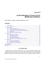
tively. The remaining unsampled reference pixels were used as validation data for assessing the
accuracy of the different methods. The cropped (ranging from 7 to 530 and from 9 to 406 pixels)
reference classification and the

G =

314 training samples used in this study are shown in Figure
11.1a and Figure 11.1b.
The class labels and the corresponding simulated reflectance values at the training sample
locations were used to derive statistical parameters: the class-conditional means
and the class-conditional (co)variances for forest, shrub, and rangeland, respectively.
The class labels of the training pixels were also used to infer the three indicator covariance models,
, for forest, shrub, and rangeland, respectively (Equation 11.5). All indicator covariance
models (not shown) were isotropic, and their parameters are tabulated in Table 11.1. The forest
and shrub indicator covariance models, , consisted of a nugget component (2 to 3% of the
total variance), a small-scale structure of practical range 25 to 30 pixels (59 to 61% of the total
variance), and a larger-scale structure of practical range 100 to 120 pixels (37 to 38% of the total
variance). The rangeland indicator covariance model, , consisted of a nugget component (1%
of the total variance), a small-scale structure of practical range 22 pixels (75% of the total variance),
and one larger-scale structure of practical range 400 pixels (24% of the total variance). These
covariance model parameters imply that forest and shrub have a very similar spatial correlation

that differs slightly from that of rangeland. The latter class has more pronounced small-scale

Figure 11.1

Reference classification (a) and 314 training pixels (b) selected via stratified random sampling.

Table 11.1 Parameters of the Three Indicator
Covariance Models,

s

1

,

s

2

,

s

3

, for Forest,

Shrub, and Rangeland, Respectively
Nugget

Sill

Range
(1) (2) (1) (2)

Forest 0.02 0.61 0.37 30 120
Shrub 0.03 0.59 0.38 25 100
Rangeland 0.01 0.75 0.75 22 400

Note:

All indicator covariances were modeled using a
nugget contribution and two exponential cova-
riance structures with respective sills and prac-
tical ranges: sill(1), sill(2), range(1), and
range(2). Sill values are expressed as a per-
centage of the total variance:

p

k

(1 –

p

k

) = 0.23,
0.17, 0.12, for forest, shrub, and rangeland,

respectively; range values are expressed in
numbers of pixels.
50 100 150 200 250 300 350 400 450 500
50
100
150
200
250
300
350
400
0 50 100 150 200 250 300 350 400 450 500
0
50
100
150
200
250
300
350
400
(a) (b)
Forest Shrub Rangeland
Forest Shrub Rangeland
+
O
mmm
XX X|| |
,,
123

SSSSSS
XX X|| |
,,
123
oo o
ssssss
123
,,
ssss
12
,
ss
3

L1443_C11.fm Page 154 Saturday, June 5, 2004 10:32 AM
© 2004 by Taylor & Francis Group, LLC

GEOSTATISTICAL MAPPING OF THEMATIC CLASSIFICATION UNCERTAINTY 155

variability, and less large-scale variability, which is also of longer range than that of forest and
shrub. For further details regarding the interpretation of variogram and covariance functions com-
puted from remotely sensed imagery, see Woodcock et al. (1988).

11.3.1 Spectral and Spatial Classifications

Using the class-conditional means and (co)variances , three
Gaussian likelihood functions were established for any vector of reflectance values at any
pixel

u

not in the training set (Equation 11.1). The three Gaussian likelihood functions were
subsequently inverted (Equation 11.2) to compute the three spectrally derived preposterior proba-
bilities, , , and , for forest, shrub, and rangeland,
respectively. These GML preposterior probabilities are shown in Figure 11.2a–c. Note (1) the high
degree of noise in the probabilities, (2) the confusion of shrub and rangeland (probabilities close
to 0.5), and (3) the motion-like appearance that entails diffuse class boundaries. The corresponding
MAP selection at each pixel

u

is shown in Figure 11.2d. Note again the high degree of fragmentation
in the classified map. The overall classification accuracy (evaluated against the reference classifi-
cation) was 0.73 (Kappa = 0.44), indicating a rather severe misclassification.
Arguably, in the presence of noise, the original spectral vector could have been replaced by a
vector of the same dimensions whose entries are averages of reflectance values within a (typically
3

¥

3) neighborhood around each pixel (Switzer, 1980). This, however, amounts to implicitly
introducing contextual information into the classification procedure: spatial variability in the reflec-
tance values is suppressed via a form of low-pass filter to introduce more spatial correlation, and
thus produce less fragmented classification maps. In the absence of noise-free data, any such filtering
procedure is rather arbitrary: there is no reason to use a 3

¥

3 vs. a 5

¥

5 filter, for example. In
this chapter, we propose a method for introducing that notion of compactness in classification via
a model of spatial correlation inferred from the training pixels themselves.
Ordinary indicator kriging (OIK) (Equation 11.5 and Equation 11.6) was performed using the
three sets of

G

training class indicators and their corresponding indicator covariance models to
compute the space-derived preposterior probabilities , , for
forest, shrub, and rangeland, respectively. These OIK preposterior probabilities are shown in Figure
11.3a–c. Note the very smooth spatial patterns and the absence of clear boundaries, as opposed
to those found in the spectrally derived posterior probabilities of Figure 11.2. Note also that the
training sample class labels are reproduced at the training locations, per the data-exactitude
property of OIK. The corresponding MAP selection at each pixel

u

is shown in Figure 11.3d. The
overall classification accuracy is 0.73 (Kappa = 0.44), the same as that computed from the
spectrally derived classification, indicating the same level of severe misclassification for the
spacially derived classification.

11.3.2 Merging Spectral and Contextual Information

Bayesian fusion (Equation 11.9), was performed to combine the individually derived spectral
and spatial preposterior probabilities into posterior probabilities ,
, and , for forest, shrub, and rangeland, respectively; these

posterior probabilities account for both information sources and are shown in Figure 11.4a–c.
Compared to the spectrally derived preposterior probabilities of Figure 11.2, the latter posterior
probabilities have smoother spatial patterns and much less noise. Compared to the spacially derived
preposterior probabilities of Figure 11.3, the latter posterior probabilities have more variable
patterns and indicate clearer boundaries. The corresponding MAP selection at each pixel

u

is shown
in Figure 11.4d. The overall classification accuracy increased to 0.80 and the Kappa coefficient to
mmm
XX X|| |
,,
123
SSSSSS
XX X|| |
,,
123
oo o
xu()
pc
1
[()| ()]uxu pc
2
[()| ()]uxu pc
3
[()| ()]uxu
pc
g1
[()| ]uc pc

g2
[()| ]uc pc
g3
[()| ]uc
pc x
g1
[()| (), ]uuc
pc x
g2
[()| (), ]uuc pc x
g3
[()| (), ]uuc

L1443_C11.fm Page 155 Saturday, June 5, 2004 10:32 AM
© 2004 by Taylor & Francis Group, LLC

156 REMOTE SENSING AND GIS ACCURACY ASSESSMENT

Figure 11.2

Conditional probabilities for forest (a), shrub (b), and rangeland (c), based on Gaussian maximum likelihood (GML), and corresponding MAP selection (d).
50 100 150 200 250 300 350 400 450 500
50
100
150
200
250
300
350
400

50 100 150 200 250 300 350 400 450 500
50
100
150
200
250
300
350
400
50 100 150 200 250 300 350 400 450 500
50
100
150
200
250
300
350
400
50 100 150 200 250 300 350 400 450 500
50
100
150
200
250
300
350
400
0
1
0. 5

0
1
0. 5
Shrub
Forest

Overall accuracy=73.4% , Kappa=43.9%
0
1
0. 5
(d)(c)
(a) (b)
Rangeland

L1443_C11.fm Page 156 Saturday, June 5, 2004 10:32 AM
© 2004 by Taylor & Francis Group, LLC

GEOSTATISTICAL MAPPING OF THEMATIC CLASSIFICATION UNCERTAINTY 157

Figure 11.3

Conditional probabilities for forest (a), shrub (b), and rangeland (c), based on ordinary indicator kriging (OIK), and corresponding MAP selection (d).
50 100 150 200 250 300 350 400 450 500
50
100
150
200
250
300
350

400
50 100 150 200 250 300 350 400 450 500
50
100
150
200
250
300
350
400
50 100 150 200 250 300 350 400 450 500
50
100
150
200
250
300
350
400
50 100 150 200 250 300 350 400 450 500
50
100
150
200
250
300
350
400
0
1

0. 5
0
1
0. 5
0
1
0. 5
(a)
(c)
(b)
(d)
Shrub
Forest

Rangeland
Overall accuracy=73.3% , Kappa=43.9%

L1443_C11.fm Page 157 Saturday, June 5, 2004 10:32 AM
© 2004 by Taylor & Francis Group, LLC

158 REMOTE SENSING AND GIS ACCURACY ASSESSMENT

0.59, a 9.6% and 34.1% improvement, respectively, relative to the corresponding accuracy statistics
computed from the GML classification.
For comparison, accuracy assessment statistics, including producer’s and user’s accuracy, for
all classification algorithms considered in this chapter are tabulated in Table 11.2. Clearly, classi-
fication accuracy using the proposed contextual classification methods was superior to that using
only spectral or only spatial information. As stated above, overall accuracy and the Kappa coeffi-
cients are significantly higher for the proposed methods. In addition, both producer’s and user’s
accuracy for all three classes are higher than the corresponding values computed from the spectrally

derived or the spacially derived classifications.
The reference and classification-derived class proportions are also provided in Table 11.3 for
comparison. Clearly, MAP selection from the fused posterior probabilities
yielded the closest class proportions to the reference ones: 0.69 vs. 0.65 (reference) for forest, 0.21
vs. 0.21 for shrub, and 0.10 vs. 0.14 for rangeland. The other methods performed worse with respect
to reproducing the reference class proportions.

11.3.3 Mapping Classification Accuracy

The three spectrally derived preposterior probabilities, , , and
for forest, shrub, and rangeland, respectively, were converted into an accuracy
value for the particular class reported at pixel

u

(i.e., for the classification of Figure 11.2d),
as described in Section 11.2.4. These accuracy values were mapped in Figure 11.5a. The same
procedure was repeated using the three fusion-based posterior probabilities ,
, and , for forest, shrub, and rangeland, respectively, to yield

Figure 11.4

Conditional probabilities for forest (a), shrub (b), and rangeland (c), based on Bayesian integration
of spectrally derived and spacially derived preposterior probabilities (GML/OIK), and corresponding
MAP selection (d).
50 100 150 200 250 300 350 400 450 500
50
100
150
200

250
300
350
400
50 100 150 200 250 300 350 400 450 500
50
100
150
200
250
300
350
400
50 100 150 200 250 300 350 400 450 500
50
100
150
200
250
300
350
400
50 100 150 200 250 300 350 400 450 500
50
100
150
200
250
300
350

400
Rangeland
Shrub
0
1
0. 5
0
1
0. 5
0
1
0. 5
(a)
(c)
(b)
(d)
Forest
Overall accuracy=79.75% , Kappa=59.26%
pc x
k
g
[()| (), ]uuc
pc
1
[()| ()]uxu pc
2
[()| ()]uxu
pc
3
[()| ()]uxu

a
c
()u
pc x
g1
[()| (), ]uuc
pc x
g2
[()| (), ]uuc pc x
g3
[()| (), ]uuc

L1443_C11.fm Page 158 Saturday, June 5, 2004 10:32 AM
© 2004 by Taylor & Francis Group, LLC

GEOSTATISTICAL MAPPING OF THEMATIC CLASSIFICATION UNCERTAINTY 159

Table 11.2 Accuracy Statistics for Classification
Based on MAP Selection from Conditional
Probabilities Computed Using Different
Methods: Gaussian Maximum Likelihood
(GML), Ordinary Indicator Kriging (OIK),
and Bayesian Integration of GML and OIK

Probabilities (GML/OIK)
GML OIK GML/OIK

Overall accuracy

0.73 0.73 0.80

Kappa

0.44 0.44 0.59

Producer’s accuracy

Forest 0.92 0.88 0.91
Shrub 0.44 0.52 0.63
Rangeland 0.30 0.39 0.51

User’s accuracy

Forest 0.82 0.78 0.86
Shrub 0.48 0.61 0.64
Rangeland 0.55 0.63 0.68

Table 11.3 Class Proportions from Reference and
Classified Maps Based on MAP Selection from
Conditional Probabilities Computed Using
Different Methods: Gaussian Maximum
Likelihood (GML), Ordinary Indicator Kriging
(OIK), and Bayesian Integration of GML and OIK

Probabilities (GML/OIK)
Reference GML OIK GML/OIK

Forest 0.65 0.73 0.73 0.69
Shrub 0.21 0.19 0.18 0.21
Rangeland 0.14 0.08 0.09 0.10

Figure 11.5

Pixel-specific accuracy values for GML-derived classes (a) and for GML/OIK-derived classes (b).
(a) (b)

L1443_C11.fm Page 159 Saturday, June 5, 2004 10:32 AM
© 2004 by Taylor & Francis Group, LLC

160 REMOTE SENSING AND GIS ACCURACY ASSESSMENT

an accuracy value for the particular class reported at pixel

u

(i.e., for the classification of
Figure 11.4d). These accuracy values were mapped in Figure 11.5b. The accuracy map of Figure
11.5b exhibited much higher values than the corresponding map of Figure 11.5a, indicating an
increased confidence in classification due precisely to the consideration of contextual information.
In addition, the low accuracy values (~0.4–0.6) of Figure 11.5b were found near class boundaries,
as opposed to the low accuracy values of Figure 11.5a, which just corresponded to pixels classified
as shrub and rangeland. This latter characteristic implied that contextual information yielded a
more realistic map of classification accuracy, which could be useful for designing additional
sampling campaigns.

11.4 DISCUSSION

A geostatistical approach for mapping thematic classification uncertainty was presented in this
chapter. The spatial correlation of each class, as inferred from a set of training pixels, along with
the actual locations of these pixels, was used via indicator kriging to estimate the location-specific

probability that a pixel belongs to a certain class, given the spatial information contained in the
training pixels. The proposed approach for estimating the above preposterior probability accounted
for texture information via the corresponding indicator covariance model for each class, as well as
for the spatial proximity of each pixel to the training pixels after this proximity was discounted for
the spatial redundancy (clustering) of the training pixels. Space-derived preposterior probabilities
were merged via Bayes’ rule with spectrally derived preposterior probabilities, the latter based on
the collocated vector of reflectance values at each pixel. The final (fused) posterior probabilities
accounted for both spectral and spatial information.
The performance of the proposed methods was evaluated via a case study that used realistically
simulated reflectance values. A subset of 0.14% (314) of the image pixels was retained as a training
set. The results indicated that the proposed method of context estimation, when coupled with
Bayesian integration, yielded more accurate classifications than the conventional maximum likeli-
hood classifier. More specifically, relative improvements of 10% and 34% were found for overall
accuracy and the Kappa coefficient. In addition, contextual information yielded more realistic
classification accuracy maps, whereby pixels with low accuracy values tended to coincide with
class boundaries.

11.5 CONCLUSIONS

The proposed geostatistical methodology constitutes a viable means for introducing contextual
information into the mapping of thematic classification uncertainty. Since the results presented in
the case study in this chapter appear promising, further research is required to evaluate the perfor-
mance of the proposed contextual classification and its use for mapping thematic classification
uncertainty over a variety of real-world data sets. In particular, issues pertaining to the type and
level of spatial correlation, the density of the training pixels, and their effects on the resulting
classification uncertainty maps should be investigated in greater detail.
In conclusion, we suggest that the final posterior probabilities of class occurrence be used in
a stochastic simulation framework, whereby multiple, alternative, synthetic representations of land
cover maps would be generated using various algorithms for simulating categorical variables
(Deutsch and Journel, 1998). These alternative representations would reproduce: (1) the observed

classes at the training pixels, (2) the class proportions, (3) the spatial correlation of each class
inferred from the training pixels, and (4) possible relationships with spectral or other ancillary
spatial information. The ensemble of simulated land-cover maps could be then used for error
a
f
()u

L1443_C11.fm Page 160 Saturday, June 5, 2004 10:32 AM
© 2004 by Taylor & Francis Group, LLC

GEOSTATISTICAL MAPPING OF THEMATIC CLASSIFICATION UNCERTAINTY 161

propagation (e.g., Kyriakidis and Dungan [2001]), thus allowing one to go beyond simple map
accuracy statistics and address map use (and map value) issues.

11.6 SUMMARY

Thematic classification accuracy constitutes a critical factor in the successful application of
remotely sensed products in various disciplines, such as ecology and environmental sciences. Apart
from traditional accuracy statistics based on the confusion matrix, maps of posterior probabilities
of class occurrence are extremely useful for depicting the spatial variation of classification uncer-
tainty. Conventional classification procedures such as Gaussian maximum likelihood, however, do
not account for the plethora of ancillary data that could enhance such a metadata map product.
In this chapter, we propose a geostatistical approach for introducing contextual information
into the mapping of classification uncertainty using information provided only by the training pixels.
Probabilities of class occurrence that account for context information are first estimated via indicator
kriging and are then integrated in a Bayesian framework with probabilities for class occurrence
based on conventional classifiers, thus yielding improved maps of thematic classification uncer-
tainty. A case study based on realistically simulated TM imagery illustrates the applicability of the
proposed method: (1) regional accuracy scores indicate relative improvements over traditional

classification algorithms in the order of 10% for overall accuracy and 34% for the Kappa coefficient
and (2) maps of pixel-specific accuracy values tend to pinpoint class boundaries as the most
uncertain regions, thus appearing as a promising means for guiding additional sampling campaigns.

REFERENCES

Atkinson, P.M. and P. Lewis, Geostatistical classification for remote sensing: an introduction,

Comput. Geosci.

,
26, 361–371, 2000.
Benediktsson, J.A. and P.H. Swain, Consensus theoretic classification methods, IEEE Trans. Syst. Man
Cybernet., 22, 688–704, 1992.
Benediktsson, J.A., P.H. Swain, and O.K. Ersoy, Neural network approaches versus statistical methods in
classification of multisource remote sensing data, IEEE Trans. Geosci. Remote Sens., 28, 540–552,
1990.
Bonham-Carter, G.F., Geographic Information Systems for Geoscientists, Pergamon, Ontario, 1994.
Congalton, R.G., A review of assessing the accuracy of classifications of remotely sensed data, Remote Sens.
Environ., 37, 35–46, 1991.
Congalton, R.G., Using spatial autocorrelation analysis to explore the errors in maps generated from remotely
sensed data, Photogram. Eng. Remote Sens., 54, 587–592, 1988.
Congalton, R.G. and K. Green, Assessing the Accuracy of Remote Sensed Data: Principles and Practices,
Lewis, Boca Raton, FL, 1999.
Cressie, N.A.C., Statistics for Spatial Data, John Wiley & Sons, New York, 1993.
De Bruin, S., Predicting the areal extent of land-cover types using classified imagery and geostatistics, Remote
Sens. Environ., 74, 387–396, 2000.
Deutsch, C.V., Cleaning categorical variable (lithofacies) realizations with maximum a-posteriori selection,
Comput. Geosci., 24, 551–562, 1998.
Deutsch, C.V. and A.G. Journel, GSLIB: Geostatistical Software Library and User’s Guide, 2nd ed., Oxford

University Press, New York, 1998.
Foody, G.M., Status of land-cover classification accuracy assessment, Remote Sens. Environ., 80, 185–201,
2002.
Foody, G.M., N.A. Campbell, N.M. Trood, and T.F. Wood, Derivation and applications of probabilistic
measures of class membership from the maximum-likelihood classifier, Photogram. Eng. Remote
Sens., 58, 1335–1341, 1992.
L1443_C11.fm Page 161 Saturday, June 5, 2004 10:32 AM
© 2004 by Taylor & Francis Group, LLC
162 REMOTE SENSING AND GIS ACCURACY ASSESSMENT
Goovaerts, P., Geostatistical incorporation of spatial coordinates into supervised classification of hyperspectral
data, J. Geogr. Syst., 4, 99–111, 2002.
Goovaerts, P., Geostatistics for Natural Resources Evaluation, Oxford University Press, New York, 1997.
Haralick, R.M. and H. Joo, A context classifier, IEEE Trans. Geosci. Remote Sens., 24, 997–1007, 1986.
Hutchinson, C.F., Techniques for combining Landsat and ancillary data for digital classification improvement,
Photogram. Eng. Remote Sens., 48, 123–130, 1982.
Isaaks, E.H. and R.M. Srivastava, An Introduction to Applied Geostatistics, Oxford University Press, New
York, 1989.
Jensen, J.R., Introductory Digital Image Processing: A Remote Sensing Perspective, Prentice Hall, Upper
Saddle River, NJ, 1996.
Journel, A.G., Non-parametric estimation of spatial distributions, Math. Geol., 15, 445–468, 1983.
Kyriakidis, P.C. and J.L. Dungan, A geostatistical approach for mapping thematic classification accuracy and
evaluating the impact of inaccurate spatial data on ecological model predictions, Environ. Ecol. Stat.,
8, 311–330, 2001.
Lee, T., J.A. Richards, and P.H. Swain, Probabilistic and evidential approaches for multisource data analysis,
IEEE Trans. Geosci. Remote Sens., 25, 283–293, 1987.
Li, S.Z., Markov Random Field Modeling in Image Analysis, Springer-Verlag, Tokyo, 2001.
Solow, A.R., Mapping by simple indicator kriging, Math. Geol., 18, 335–352, 1986.
Steele, B.M., Combing multiple classifiers: an application using spatial and remotely sensed information for
land cover type mapping, Remote Sens. Environ., 74, 545–556, 2000.
Steele, B.M. and R.L. Redmond, A method of exploiting spatial information for improving classification rules:

application to the construction of polygon-based land cover type maps, Int. J. Remote Sens., 22,
3143–3166, 2001.
Stehman, S.V., Comparing thematic maps based on map value, Int. J. Remote Sens., 20, 2347–2366, 1999.
Stehman, S.V., Selecting and interpreting measures of thematic classification accuracy, Remote Sens. Environ.,
62, 77–89, 1997.
Strahler, A.H., Using prior probabilities in maximum likelihood classification of remotely sensed data, Remote
Sens. Environ., 47, 215–222, 1980.
Swain, P.H., S.B. Vardeman, and J.C. Tilton, Contextual classification of multispectral image data, Pattern
Recogn., 13, 429–441, 1981.
Switzer, P., Extensions of linear discriminant analysis for statistical classification of remotely sensed data,
Math. Geol., 12, 367–376, 1980.
Switzer, P., W.S. Kowalik, and R.J.P. Lyon, A prior method for smoothing discriminant analysis classification
maps, Math. Geol., 14, 433–444, 1982.
Tso, B. and P.M. Mather, Classification Methods for Remotely Sensed Data, Taylor & Francis, London, 2001.
van der Meer, F., Classification of remotely sensed imagery using an indicator kriging approach: application
to the problem of calcite-dolomite mineral mapping, Int. J. Remote Sens., 17,1233–1249, 1996.
Vogelmann, J.E., T.L. Sohl, P.V. Campbell, and D.M. Shaw, Regional land cover characterization using Landsat
Thematic Mapper data and ancillary data sources, Environ. Monit. Assess., 51, 415–428, 1998.
Woodcock, C.E., A.H. Strahler, and D.L.B. Jupp, The use of variograms in remote sensing. I: scene models
and simulated images, Remote Sens. Environ., 25, 323–348, 1988.
Zhang, J. and M. Goodchild, Uncertainty in Geographic Information, Taylor & Francis, London, 2002.
L1443_C11.fm Page 162 Saturday, June 5, 2004 10:32 AM
© 2004 by Taylor & Francis Group, LLC