Motion Control 2009 Part 7 ppt
Bạn đang xem bản rút gọn của tài liệu. Xem và tải ngay bản đầy đủ của tài liệu tại đây (7.01 MB, 35 trang )
Motion Control
202
increased with increasing frequency and amplitude, the active body length involved in the
swimming increased continually because of the participation of more joints. Nevertheless,
all the joints functioned and the active body length remained invariant in the second stage.
The two-phase profile demonstrated that the oscillating body length plays an important role
in the swimming speed of the AmphiRobot.
(a) drive=1
(b) drive=1.5
Terrestrial and Underwater Locomotion Control for
a Biomimetic Amphibious Robot Capable of Multimode Motion
203
(c) drive=2
(d) drive=2.5
Fig. 19. A comparison of actual swimming and simulation results
Motion Control
204
Fig. 20. The relationship of swimming speed and drive difference
5. Conclusion
This chapter has reviewed some of the issues involved in creating a multimode amphibious
robot, especially its mechanical design and motion control, in a biomimetic manner. Based
on the body structure, motion characteristics of amphibians, two generations of multimode
biomimetic amphibious robots, named “AmphiRobot”, have been developed. For terrestrial
movements, a geometry based steering method called body-deformation steering has been
proposed and optimized, taking advantage of the wheel-like mechanisms attached to the
robot. At the same time, a chainlike CPG network responsible for coordinated swimming
between multi-joint tail and artificial pectoral fins has been built. The aquatic control
parameters mainly involve the length of undulation part, oscillating frequency and
amplitude cooperatively regulated by the threshold values of the saturation function for
each propelling unit. The real-time online calculation of controlling parameters has been
also implemented. Preliminary testing results, both on land and in water, have
demonstrated the effectiveness of the proposed control scheme. However, the amphibious
locomotion performance of the AmphiRobot is still far behind that of animals in terms of
speed and agility, especially in complex unstructured environments. More cooperative
efforts from materials, actuators, sensors, control as well as learning aspects will be needed
to improve the robot locomotor skills in unstructured and even unknown surroundings.
The ongoing and future work will focus on the analysis and optimization of locomotion
control for autonomous movements as well as flexible water-land transitions.
Hydrodynamic experiments based hybrid mechanical/electrical optimization, of course, is a
plus for real-world applications.
6. Acknowledgement
The authors would like to thank Prof. Weibing Wang in the Machine and Electricity
Engineering College, Shihezi University, for his contribution to mechanical design and
fabrication of the AmphiRobot.
Terrestrial and Underwater Locomotion Control for
a Biomimetic Amphibious Robot Capable of Multimode Motion
205
This work was supported in part by the National Natural Science Foundation of China
under Grants 60775053 and 60505015, in part by the Municipal Natural Science Foundation
of Beijing under Grant 4082031, in part by the National 863 Program under Grant
2007AA04Z202, and in part by the Beijing Nova Programme (2006A80).
7. References
Ayers, J. (2004). Underwater walking, Arthropod Structure and Development, Vol. 33, pp. 347–
360
Bandyopadhyay, P.R. (2004). Guest editorial: biology-inspired science and technology for
autonomous underwater vehicles, IEEE J. Ocean. Eng., Vol. 29, No. 3, pp. 542–546
Bandyopadhyay, P.R. (2005). Trends in biorobotic autonomous undersea vehicles, IEEE J.
Ocean. Eng., Vol. 30, No. 1, pp. 109–139
Barrett, D.S. (1996). Propulsive efficiency of a flexible hull underwater vehicle, Dissertation
for the Doctoral Degree, Cambridge, MA: Massachusetts Institute of Technology
Boxerbaum, A.; Werk, P.; Quinn, R. & Vaidyanathan, R. (2005). Design of an autonomous
amphibious robot for surf zone operation: Part I mechanical design for multi-mode
mobility, Proc. of the 2005 IEEE/ASME International Conference on Advanced Intelligent
Mechatronics, pp. 1460–1464
Delcomyn, F. (1980). Neural basis for rhythmic behaviour in animals, Science, Vol. 210, pp.
492–498
Ding, R.; Yu, J.; Yang, Q.; Hu, X. & Tan, M. (2009). Platform-level design for a biomimetic
amphibious robot, Proc. of IEEE International Conference on Robotics and Biomimetics,
Bangkok, Thailand, pp. 977–982
Fish, F.E. & Rohr, J.J. (1999). Review of dolphin hydrodynamics and swimming
performance, Technical Report 1801, SPAWARS System Center San Diego, CA
Georgiades, C.; Nahon, M. & Buehler, M. (2009). Simulation of an underwater hexapod
robot, Ocean Engineering, Vol. 36, pp. 39–47
Greiner, H.; Shectman, A.; Won, C.; Elsley, D. & Beith, P. (1996). Autonomous legged
underwater vehicles for near land warfare, Proc. Symp. Autonom. Underwater Vehicle
Tech., pp. 41–48
Harkins, R.; Ward, J.; Vaidyanathan, R.; Boxerbaum, A. & Quinn, R. (2005). Design of an
autonomous amphibious robot for surf zone operation: Part II - hardware, control
implementation and simulation, Proc. of the 2005 IEEE/ASME International
Conference on Advanced Intelligent Mechatronics, pp. 1465–1470
Healy, P.D. & Bishop, B.E. (2009). Sea-dragon: an amphibious robot for operation in the
littorals, Proc. of 41st Southeastern Symp. on System Theory, University of tennessee
Space Institute, Tullahome, TN, USA, pp. 266–270
Ijspeert, A.J.; Crespi, A. & Cabelguen, J M. (2005). Simulation and robotic studies of
salamander locomotion: applying neurobiological principles to the control of
locomotion in robots, Neuroinformatics, Vol. 3, pp. 171–196
Ijspeert, A.J.; Crespi, A.; Ryczko, D. & Cabelguen, J M. (2007). From swimming to walking
with a salamander robot driven by a spinal cord model, Science, Vol. 315, No. 5817,
pp. 1416–1420
Ijspeert, A.J. (2008). Central pattern generators for locomotion in animals and robots: a
review, Neural Networks, Vol. 21, No. 4, pp. 642–653
Motion Control
206
Kemp, M.; Hobson, B. & Long, J. (2005). Madeleine: an agile auv propelled by flexible fins,
Proc. of the 14th International Symposium on Unmanned Untethered Submersible
Technology (UUST), pp. 1–6
Lauder, G.V.; Anderson, E.J.; Tangorra, T.J. & Madden, P.G.A. (2007a). Fish biorobotics:
kinematics and hydrodynamics of self-propulsion, The Journal of Experimental
Biology, Vol. 210, pp. 2767–2780
Lauder, G.V. & Madden, P.G.A. (2007b). Fish locomotion: kinematics and hydrodynamics of
flexible foil-like fins, Exp. Fluids, Vol. 43, pp. 641–653
Prahacs, C.; Saunders, A.; Smith, M.; McMordie, D. & Buehler, M. (2005). Towards legged
amphibious mobile robotics, J. Eng. Design and Innovation (online), vol. 1, part. 01P3,
Available: www.cden.ca/JEDI/index.html
Sfakiotakis, M.; Lane, D.M. & Davies, J.B.C. (1999). Review of fish swimming modes for
aquatic locomotion, IEEE J. Oceanic Eng., Vol. 24, No. 2, pp. 237–252
Yamada, H.; Chigisaki, S.; Mori, M.; Takita, K.; Ogami, K. & Hirose, S. (2005). Development
of amphibious snake-like robot ACM-R5, Proc. of 36th Int. Symposium on Robotics,
pp. 433–440
Yang, Q.; Yu, J.; Tan, M. & Wang, S. (2007). Amphibious biomimetic robots: a review, Robot,
Vol. 29, No. 6, pp. 601–608
Yu, J.; Tan, M.; Wang, S. & Chen, E. (2004). Development of a biomimetic robotic fish and its
control algorithm, IEEE Trans. Syst., Man, Cybern. B, Cybern., Vol. 34, No. 4, pp.
1798–1810
Yu, J.; Hu, Y.; Fan, R.; Wang, L. & Huo, J. (2007). Mechanical design and motion control of a
biomimetic robotic dolphin, Advanced Robotics, Vol. 21, No. 3–4, pp. 499–513
Wang, L.; Sun, L.; Chen, D.; Zhang, D. & Meng, Q. (2005). A bionic crab-like robot
prototype, Journal of Harbin Engineering University, Vol. 26, No. 5, pp. 591–595
10
Autonomous Underwater Vehicle
Motion Control during Investigation of
Bottom Objects and Hard-to-Reach Areas
Alexander Inzartsev, Lev Kiselyov,
Andrey Medvedev and Alexander Pavin
Institute of Marine Technology Problems (IMTP FEB RAS)
Far East Branch of the Russian Academy of Sciences
Russia
1. Introduction
Modern Autonomous Underwater Vehicles (AUVs) can solve different tasks on sea bosom
research, objects search and investigation on the seabed, mapping, water area protection,
and environment monitoring. In order to solve problems of bottom objects survey AUV has
to move among the obstacles in a small distance from the seabed. Such motion is connected
with active manoeuvring, changes in speed and direction of the movement, switch and
adaptive correction of modes and control parameters. This can be exemplified by using
AUV for geologic exploration and raw materials reserves estimation in the area of
seamounts, which are guyots with rugged topography. Such problems arise during vehicle
manoeuvring near artificial underwater point or extended objects (for example, dock
stations or underwater communications). The problems of ocean physical fields’ survey are
of a particular interest. These are the problems of bathymetry and seabed mapping as well
as signature areas of search objects.
To perform these tasks AUV must be equipped with the systems that can define the
positions of the vehicle body against the obstacles and search objects. As a rule, acoustic
distance-measuring systems (multibeam and scanning sonars, and also groups of sonars
with the fixed directional diagram) and other vision systems are used for these purposes.
AUV path planning is carried out with the use of current sensory data due to the lack of a
priori information. On the basis of measured distances the current environment model and
the position of the vehicle are defined. Then taking into account vehicle dynamic features
the direction of probable movement and usable motion modes are evaluated. At each
control phase a motion replanning is carried out taking into account new data received from
sensors and changed surrounding.
The paper presents the results of research and working outs based on the many years of
experience of the Institute of Marine Technology Problems (IMTP) FEB RAS (Ageev et al.,
2005). It also gives examples of realization of the offered solutions in the structure and
algorithms of motion control of certain autonomous underwater vehicles-robots.
Motion Control
208
2. Control system peculiarities of AUV capable to work at severe environment
The use of AUV to perform different operations under conditions of difficult informative
uncertain or extreme surrounding requires a developed complex of positioning, control, and
computer vision systems onboard the vehicle. In the overall structure of control system one
can mark such basic systems providing AUV functioning as an equipment carrier, and
information and searching functions.
The basis of control system is a local area network composed of several computers. It
provides motion control and emergency and search functions. To organize AUV’s local area
network high speed channels (Ethernet) and quite slow exchange serial channels are used.
To form the control navigation and sensors’ data are used. Emergency sensors are used for
AUV safety. Remote change of AUV mission can be carried out with the help of acoustic
link. Positioning system plays an important role. Positioning accuracy is acquired by using
on-board autonomous navigation system including inertial positioning system, angular and
position measuring devices, and acoustic Doppler log. An accumulating dead-reckoning
error can be decreased by means of integration of hydroacoustic and stand-alone data by
operating AUV with hydroacoustic navigation facilities with long or ultra-short base.
Search systems incorporated computer vision systems differ on physical principles and
methods of data acquisition. Acoustic systems include high-frequency and low-frequency
side-scan and sector-scan sonars as well as subbottom profiler. Current-conducting objects
can be found with the use of electromagnetic locator (EML). A video system carries out
imaging and object recognition. It includes photo and video cameras.
The information from sensors and measuring systems are usually stored for the following
mapping of researched area (ecological, geophysical, etc.) If necessary, this information can
be used in real time, for example, for contouring the areas with abnormal characteristics of
measured fields.
System architecture of programmed control has hierarchic three-level organization
(strategic, tactic and executive levels). Program-task (mission) for the vehicle is programmed
on the highest level and in general it contains the description of desired motion path and
operation modes of onboard equipment. Tactic level contains a set of vehicle behavior
models (function library) and a scheduler that coordinates their work. The lowest level
carries out tactical commands. To do this it contains a set of servocontrollers. Control
algorithms providing “reflex” motion among the obstacles work on the lowest level.
The propulsion system is used for spatial motion, positioning, and obstacle avoiding. It
provides free motion modes (motion in wide speed range, hovering, and free trim motion).
There are stern and bow propulsion sections. Control forces and moments are created with
the help of four stern mid-flight and several stern and fore lateral thrusting propulsions.
Multi-beam echoranging system (ERS) with the range up to 75 meters is used for working
out corresponding controls and obstacles detection. ERS sonars are oriented on the front
aspect under different angles to vehicle fore-and-aft axis (forward, down, sideway, up).
3. Motion modes and AUV dynamics peculiarities
Trajectories of arbitrary forms are required for bottom objects survey, constructions
inspection, docking with mooring facilities or homing beacons. Not only basic motion
modes but more difficult modes of dynamic positioning at variable speed and circular
change of thrust vector direction (start-stop, reverse, transversal, etc.) must be performed.
Among typical practical tasks of this class are:
Autonomous Underwater Vehicle Motion Control during Investigation
of Bottom Objects and Hard-to-Reach Areas
209
• maneuvering in specified area near the target at variable speed and heading correction,
pointing to the target (signal source), approaching to the target and point positioning,
• lengthy objects search and survey,
• path selection in the rugged bottom relief.
In many cases the said missions are interconnected and can correspond to different phases
of a particular vehicle mission. So we shall consider them as components of single scenery
for rather complex missions’ performance.
Fig. 1. A system of coordinates and flow pattern of force in trimetric projection
Let’s equate the model of AUV spatial motion as (fig. 1):
0
11 22 33
sin cos cos cos sin ,
cos cos cos ,
sin ,
,
cos cos ,
sin ,
sin cos .
,,,
xx x y z
yy x y
ctrl
zz z
ctrl
yyy
Tx
Ty
Tz
xy z
mRP T T T
mRP T T
JMM M
JMM
X
Y
Z
mM mM mM I
υ
ϑαβαβ
υϑ ϑ α α
ψψ
ϕ
υϑϕυ
υϑυ
υϕϑυ
λλ λ
=− + ⋅ + ⋅ ⋅ − ⋅ − ⋅
=+⋅ +⋅ +⋅
=+⋅ +
=+
=⋅ ⋅ +
=⋅ +
=⋅ ⋅ +
=+ =+ =+
55 66
,,
yyy zzz
III
λ
λ
=+ =+
(1)
where
λ
11
,
λ
22
,
λ
33
,
λ
55
,
λ
66
– added masses and liquid inertia moment, T
x1
, T
y1
, T
z1
, M
y
ctrl
,
M
z
ctrl
– projection of control forces and moments in a system of coordinates dependent on
the vehicle,
υ
- speed against the flow, φ, ψ – heading and vehicle pitch correspondingly,
ϑ
,
χ
– angles of ascent and motion swing, R
x
, R
y
, R
z
, M
y
, M
z
– hydrodynamic forces and
moments, M
0
– moment of stability,
υ
Tx
,
υ
Ty
,
υ
Tz
– current velocity vector components which
Motion Control
210
have constant, variable or random character, P – variable buoyancy depending, in
particular, on the depth of the vehicle descent.
According to the general formulation area survey is performed with the help of
maneuvering piecewise-constant speed and path program near the target (object) and start-
stop control mode at point dynamic positioning or along the contour.
Horizontal motion area (X, Z) can be defined by one of the following methods:
• coordinates of the target point {X
T
, Z
T
}, local area radius r
T
and distance to the target d
T
,
distance d
B
to the signal source (transponder) and bearings ϑ
B
,
• optional close circuit g(X,Z)=0, against which the vehicle displacement d
i
is defined in
directions dependent of the vehicle,
• linear zone |aX+bZ+c| ≤ Δ
l
width Δ
l
against extended object and relative linear
{ΔX
l
,ΔZ
l
} and angular Δϕ
l
vehicle motions.
Control responses created by the stern and bow propulsions in the trimetric projection
connected with the vehicle are given by (Ageev et al., 2005; Kiselev & Medvedev, 2009):
()cos,
()sin ,
( ) sin ,
( )( sin cos ) ,
()(sincos) ,
x SUSRSBSL
S
ySUSB BHyBV
S
zSRSL BVzBH
ctrl S
z
SU SB BV TB y BV TB
ctrl S
ySRSLTS TS BHTBz BHTB
TS TS
TTTTT
TTT TTT
TTT TTT
M
T Tx y Tx TdTx
MTTx z TxTdTx
d
δ
δ
δ
δδ
δδ
=+++⋅
=−⋅+=+
=−⋅ +=+
=− + +⋅=⋅+⋅
=− + +⋅=⋅+⋅
=
max max
max max
( sin cos ) sin ,
,.
TS TS TS TS
SB
TT
B
S
SB
B
S
xy xyctg
UU
TT sat TT sat
TT
δδδ δ
⋅+⋅ =+⋅
⎛⎞
⎛⎞
=⋅ =⋅
⎜⎟
⎜⎟
⎝⎠
⎝⎠
(2)
where Т
SU
, Т
SB
– vertical channel stern mid-flight propulsions thrusts (upper and bottom
correspondingly), Т
SR
, Т
SL
- horizontal channel stern mid-flight propulsions thrusts (right
and left correspondingly), Т
BH
, Т
BV
- horizontal and vertical bow maneuvering thrusts, х
TS
,
у
TS
,
δ
- coordinates and pitch angle of stern mid-flight propulsions, х
TB
- axial coordinate of
bow maneuvering propulsion, U
S
T
, U
B
T
- control functions for stern and bow propulsion
sections.
As is clear from set of equations one and the same control responses can be created by
means of applying different work patterns of stern and bow propulsions. A practical
application has the following modes:
• cruising motion;
• low speed motion.
The first mode is characterized by the fact that vehicle spatial motion is carried out by
means of changing of attack angle with the help of variables T
x
, M
Y
CTRL
, M
Z
CTRL
. At the same
time only stern mid-flight propulsions form the mentioned forces and moments. This mode
is used for vehicle control only at cruising speed.
Autonomous Underwater Vehicle Motion Control during Investigation
of Bottom Objects and Hard-to-Reach Areas
211
In the second mode all propulsion sections are used to form vehicle motion, and control is
performed according to five degrees of freedom with the help of variables T
x
, T
Y
, T
Z
, M
Y
CTRL
,
M
Z
CTRL
. This mode is used for vehicle control at low speed and during hovering.
Complex AUV motions are carried out by means of combination of these two modes. Let’s
analyze several possible control methods. They differ by the logic of program algorithm and
by system dynamics in performing complex spatial motions.
4. Motion control in the rugged bottom relief
AUV usage for seabed layer survey is connected with the organization of equidistant motion
(motion at equally distance from the seabed) and bypassing or bending around the
obstacles. Equidistant motion control assumes the formation of an equidistant model on the
basis of echoranging data and data on vehicle relative motion. In this case control can be
organized as an adjusted program that can forecast spatial equidistant path and direct the
vehicle along it. In a plane case the task is simplified and consists in stabilization of
positioning and angular error formed with the help of several range sensors. Such control
method was implemented in different versions of the majority of the vehicles designed by
IPMT FEB RAS (Ageev et al., 2005).
Characteristic features of the task can be illustrated on the example of control organization
during seamounts (guyots) survey. They are distinguished by sharp changeable microrelief
and different obstacle along the motion path (Ageev et al., 2000; Smoot, 1989). AUV use for
seamounts survey is mainly connected with the geologic exploration and raw materials
reserves estimation (for example, the resources of ferro-manganese nodules in the Pacific
Ocean created on the guyots tilted areas). Common characteristics of the guyot macrorelief are:
• cone form with side angle up to 30°- 40° near the top;
• flat top covered with the fall-outs, the edge can have barriers;
• nodules are created in the guyot upper vein systems;
• sides and top can have picks and gorges;
• side can have terraces (width up to several kilometers), edges can have peaks and
barriers.
The main objective of the survey is the estimation of amount of minerals in the given area
and the conditions for the following exploitation. The second task in using AUV is reduced
to SSS survey. The first task can be partly solved by using photo and TV survey. It is a rather
complicated task because it is quite difficult due to the necessity to approach to the surface
up to 3-5 meters.
Let’s consider potential obstacles in more detail.
Peaks are rather large underwater mounts with pike. The vehicle must pass such obstacles
sideways.
Barriers and peaks can be found on terrace edges and guyot top edge. Fault ridge height can
be up to dozen of meters. Bypassing of low barrier is rather simple. Peak bypassing during
moving from below is a more complicated task. In this case the vehicle has to stop forward
motion and emerge staying at an allowable distance from the obstacle.
Breaks and gorges are not the survey objects and the vehicle must go above them. The major
problem is to recognize this land shape.
Let’s consider several motion peculiarities in typical mode taking into account dynamic
features of the vehicle and power requirements. Broadly speaking, the selection of motion
modes is rather optional. The following variants are possible:
Motion Control
212
• motion along the side with zero pitch or with the pitch that corresponds the side angle;
• obstacle bending “without a pause” at permanent or variable speed;
• deceleration or back motion with transfer to hovering when the obstacle that cannot be
bypassed “without a pause” is found;
• body scanning without forward motion for obstacle heighting and maximal visual
angle;
• complex obstacle avoiding (peak, high hurdle) with the use of backward motion at big
pitch and attack angle.
It is necessary to choose the most energetically efficient motion modes. So the modes with
absolute minimum resistance are more preferable. It is connected with providing an
“optimal” angle of attack that corresponds preset current speed. Not all of the
abovementioned modes meet this requirement. So, moving along the side with zero pitch
cannot be considered appropriate as the basic mode, as in this case there can be high angles
of attack, and energy consumption can be reduced only at the expense of speed decreasing.
In just the same way it is difficult to provide energetically efficient mode at complicated
maneuvering near the obstacle as vehicle security prioritizes. As a consequence there
appears additional energy consumption for motion performing. One more peculiarity is
incomplete, unreliable, fuzzy information about the bottom configuration. It leads to the
suitability of construction of hybrid control structure with fuzzy-logic elements (Ageev et
al., 2000; Kiselev & Medvedev, 2009). Let us cite as an example the results of motion
modeling in vertical plane for such typical control modes as obstacle bending “without a
pause” at equidistant curve with regard to relief, bending around high and rapid obstacles,
maneuvers on tracking another more complicated bottom forms.
For descriptive reasons sonar beams are depicted at several points of motion path. The
length of each beam corresponds to ERS radius of action. In most cases complicated
obstacles bending is carried out with the use of deceleration and back motion modes. In all
considered cases control system keeps equidistant motion at preset distance of 3 meters.
When the obstacle is found it performs maneuver on its avoiding. The use of fuzzy-logic
elements with failures in ERS work allows leveling equidistant motion path, especially at
unreliable information intensification.
4.1 Motion along the side with preset pitch
The mostly widespread case during guyots’ research is moving along the smooth slope.
Creation of control forces and moments with the help of four stern and one bow propulsions
gives a chance for free selection of propulsion thrust values betweenness. In particular, if
vertical force Т
Y
and moment М
z
are defined, then it is possible to find the equations for all
thrust components at presence of all additional kinematical connections from static
equations. At the same time with the purpose of energy minimization it’s possible to let that
depth stabilization and motion along smooth lope is carried out at cruising mode (with the
use of mid-flight propulsions), and during maneuvering and moving along steep slope stern
and fore propulsions work simultaneously.
Actual angle of attack is defined by correlation of vertical thrust components, buoyancy, and
uplift hydrodynamic force. As the last one nonlinearly depends on speed and angle of
attack, it is obvious that power spent for motion is also in nonlinear dependence of angle of
attack. This can be approximately evaluated on the basis of empirical data.
Autonomous Underwater Vehicle Motion Control during Investigation
of Bottom Objects and Hard-to-Reach Areas
213
4.2 Various obstacle bending
For single obstacles avoiding such as “bench”, “hurdle”, “den”, “cutting”, and so on, typical
control based on the echoranging data can be used.
When the obstacle is found a pitch that is corresponding its height is created. Vehicle
dynamic features and control character are analogous to the previous case. Besides, safety
distance is under control. It allows obstacle bending “without a pause” and without
deceleration as well as bow propulsion switching on.
The motion mode is chosen depending on slope gradient Δ calculated on the basis of ERS
data at each points of motion path.
Let d
i
(i = 1 4) – is rangers’ distances directed correspondingly down, at an angle, forward,
and at an angle upward;
α
i
, - angle between i and i +1 ranger, i
ϕ
i
– angle between vehicle
fore-and-aft axis and i- th ranger,
ψ
- pitch. Then slope gradient is calculated as follows:
3
1
1
1
1
sin
max , (90 )
sin
i
o
ii
iiik
i
k
ii i
d
arctg
dd
α
ψ
ϕϕαα
α
+
=
=
+
⎛⎞
⎛⎞
⋅
Δ= + − = − +
⎜⎟
⎜⎟
⎜⎟
−⋅
⎝⎠
⎝⎠
∑
(3)
Median filtering is used to eliminate influence of rangers’ noise on calculated slope.
Let
δ
1
and
δ
2
are slope gradient threshold values at which the switch from cruising motion
mode to the deceleration or stern propulsion mode takes place. At small slope gradient
(|Δ|<
δ
1
) a cruising motion mode at the speed of υ ≈1 m/s is used. This mode is provided by
the work of vehicle stern propulsions.
Fig. 2. Obstacle bending: “without a pause” (left) and high “hurdle” (right)
To form control М
z
positional error dY=Y
T
– min(d
1
, d
2
соsα) (here Y
T
– preset height over
the bottom), program pitch in the shape of calculated surface steep Δ, angular speed on
pitch ψ′, and safety distance on the front ranger d
3
are used:
(
)
12 343
() 1
z
M
KdY K K K d
ψψ
=⋅+⋅Δ−+⋅+⋅
(4)
At the same time small obstacles are bended “without a pause”. Fig. 2 (left) shows the
example of obstacle bending when its height is compared with the height of vehicle motion.
It depicts motion path and positions of the casing at every 20 seconds of simulation time.
The width of coordinate grid square side is 10 m.
At large slope gradient (
δ
1
<|Δ|<
δ
2
) vehicle speed reduces up to 0.5 m/s. To create control
moments the collaboration of stern and fore propulsions is used. It allows creating much
larger trim angles.
Motion Control
214
To avoid high and rapid obstacles (|Δ|>
δ
2
) vehicle stops its forward motion and keeps
allowable distance to the obstacle. Upon that the distance to the obstacle is controlled
according to the upper and front rangers. Simultaneously upward motion on the slope with
pitch stabilization takes place. Fig. 2 (right) shows the example of “hurdle” obstacle
bending.
Control thrusts and moments are formed as follows:
(
)
134 2
max
14 2
12
min( , ) ,
,
90
2, 90
,,
90
30,
90
(2) ,
(-)
z
o
o
y
T
y
o
o
T
zT
TK dd DKx
T
Y
TD
Kd Y K
MK K
ψ
ψψ ψ
=⋅ −+⋅
⎧
≤
⎧
≤
Δ
Δ
⎪⎪
==
⎨⎨
>
Δ
⋅− +⋅ >
Δ
⎪
⎪
⎩
⎩
=⋅ +⋅
(5)
where К
1
, К
2
– are control parameters,
ψ
T
– target pitch.
As distinct from previous case AUV cannot perform bending of such an obstacle “without a
pause” due to its great height.
At point “A” vehicle decelerates and starts stabilizing preset distance to the obstacle. This
distance is in proportion to preset motion height. Vehicle deceleration is performed
smoothly due to timely obstacle detection.
4.3 Complicated obstacles avoiding
A slope with gradient of 90° and more is considered to be “peak” or “cave” obstacle. The
stabilized distance to the obstacle increases up to 30÷40 m. It brings to backward motion
under the “peak”, or to the fact that the vehicle doesn’t enter the “cave”. Fig. 3 shows the
example of vehicle motion in the area of such an obstacle. The size of the obstacle is so that it
is fully in the field of ERS vision. On the basis of this data vehicle emerges without entering
into the “cave”.
Fig. 3. “Cave” obstacle bending (left figure) and “peak” obstacle bending (right figure)
Obstacle bending of such type is characterized by the use of deceleration and backward
motion modes. The angle of attack can vary up to 180°. Fig. 3 (right) shows the example of
vehicle motion under the “peak”. This case is similar to the one described above. The only
difference is that AUV cannot beforehand estimate the character of the obstacle due to its
Autonomous Underwater Vehicle Motion Control during Investigation
of Bottom Objects and Hard-to-Reach Areas
215
great size. As a result only at point “A” a vehicle can define that it is under the “peak” and
starts backward motion.
This motion algorithm allows avoiding getting into the “gorges” if their width is compared
to the ERS radius of action.
The example of AUV upward motion on the slope with rather rugged relief is depicted in
fig. 4.
Fig. 4. Rugged relief motion
The whole motion path consists of several areas. Each area has its own motion mode. AUV
preset motion height over the bottom is 3 m. Areas 1,2,4,5 are represented as the motion
modes along the slope that has both positive and negative steep from 70° to -65°. At area 3
the vehicle performs “peak” bending. Motion at great distance from the slope at this area is
explained by the fact that “peak” in the motion direction was found beforehand. At area 6
the vehicle performs exit from under the “peak” of a greater size in the same way as it was
described earlier.
5. Extended objects search and tracking
Characteristic feature of the task is in organization of extended line search according to the
AUV systems signals for the following object tracking in the given survey zone (Ageev et al.,
2005; Inzartsev & Pavin, 2009). Practical approaches to perform such task with the use of
echosounder (Inzartsev & Pavin, 2006; Pavin, 2006), magnetometric, electromagnetic
(Kukarskih & Pavin, 2008) and video (Scherbatyuk et al., 2000) systems are known. Such
decisions were used in AUVs “AE-2”, “XP-21”, and “R-1”. Motion control is formed by
means of choosing general direction and its correction according to the contact with the
object. In fuzzy situations search motions are performed in limited area.
When the object is found vehicle linear and angular motion parameters with regard to
extended line are defined. These parameters are an input data for AUV control system. The
task is to make so that the AUV trajectory “in average” to be as close to the tracked object as
possible in the presence of positioning and dynamic errors.
Motion Control
216
If location of extended object is defined beforehand with preciseness enough for coming of
the vehicle into the point of contact establishing with the detecting devices, then the vehicle
mission includes:
• arrival to the object area and contact search with the object;
• maneuvering near the object and detecting of extended line orientation;
• extended line tracking at given “zone” that corresponds the area of steady state contact;
• return to the search program at occasional loss of contact with the object.
Acquisition system can include different devices that allow finding the object according to
the short-range signals and identify it against the background of false signals. To solve this
problem the computer video system must include high-resolution survey sonars, video
system and magnetometric or electromagnetic detecting devices.
Let’s illustrate general provisions on the example of underwater cable inspection with the
use of video system and electromagnetic locator designed by IPMT FEB RAS. Fig. 5 shows
the layout of devices used by AUV.
Fig. 5. AUV coordinates and devices layout
When the object is found with the help of video system at the output of recognition system
for each frame the following set of values is pointed out:
• direction of recognized extended object with regard to image fore-and-aft axis;
Autonomous Underwater Vehicle Motion Control during Investigation
of Bottom Objects and Hard-to-Reach Areas
217
• distance from the center of the frame to the linear object;
• length of visible part of the object.
Received parameters are used to define the position of the object in inertial system of
coordinates.
In the mode of object tracking the control data is formed as:
()
,
,
( , ) | sin( ) | .
tag AUV line
tag line p Y d Y
tag tag VIC v tag
sat K d K d
vfht K
ϕ
ϕϕ
αϕ
α
=
+Δ
=Δ ⋅ ⋅Δ + ⋅
=+⋅
(6)
Where:
Δϕ
line
- object orientation in the system of coordinates connected to the camera;
K
p,
K
d
- amplification constants for positional and differential components;
K
ν
- constant of proportionality;
α
tag
- target attack angel;
Δ
d
Y
- preset position stabilization error in diametral plane,
d
•
Y
- AUV motion speed in cross direction;
f(h
tag
,t
VIC
) - function evaluating dependence of preset AUV speed from the motion height
and operational period of video image processing system.
Extended object position according to the data of electromagnetic detecting system is
defined at the moment of maximum potentials on receiving electrodes. Estimated
Fig. 6. Cable tracking with the use of on EML (upper figure), EML and video system (central
figure), only video system (lower figure)
Motion Control
218
probability of the search object existence is defined on the basis of the values of potential
and speed of its increasing for the period of time preceding the maximum. Particular
dependence is chosen empirically on the basis of device characteristics, AUV velocity (and
height), and inspected object characteristics (electromagnetic characteristics, diameter, shell
thickness and so on).
At coprocessing of video, electromagnetic and navigation signals the control of the contacts
with the object is performed, and the data for AUV control system is worked out (Inzartsev
& Pavin, 2008). Fig. 6 shows the graphs illustrating the process of cable tracking at separate
and joint use of electromagnetic locator and video system.
6. Guiding to the given target in the action of disturbances
Let’s analyze the task of AUV motion control in conditions of incomplete or unreliable
information about environment and action of shift current. To be more specific let’s dwell
upon the analysis of vehicle motion in guiding to the given target from random starting
position. This task can be considered as a component of the closing-in scenario and coupling
with underwater target.
In this case it is necessary to provide approach and hovering of the vehicle above the object
(at the target) in the dynamic positioning mode. Guiding algorithm can use information
received from navigation-piloting sensors and positioning system data on the vehicle
coordinates, pointing to the target and distance to it. AUV motion control is conducted by
transformation of control forces and moments into the thrusts, its calculated by the program
and created by thrust-steering complex.
In general the algorithm must provide:
• classification of incalculable attack moments to work out adequate behavior;
• current vector autodetection with sufficient accuracy to compensate crabbing in
stabilization tasks;
• behavior shaping based on the history of AUV and control algorithm conditions.
Let’s call R
1
– area radius where guiding to the target is performed, R
0
– maneuvering area
radius, R – distance from vehicle to target.
Under conditions of constant current the following mode of vehicle approaching to the
target is logical:
• motion on bearings (azimuth) of the target on preset constant speed at R>R
1
,
• speed reduction at signing on the area R
0
≤R≤R
1
and turn into the direction
corresponding to the bearings sign (or value),
• position stabilization at R<R
0
.
While moving into given small area program algorithm logic forms speed change mode,
relative bearing ϕ
k
and turn directions:
1
,,
(), ,
()( ).
kkg
k
kk kkg
kk kg k g
rr
s
ign r r
arctg Z Z X X
ϕ
ϕ
ϕϕ ε
εϕ
+
≤
⎧
⎪
=
⎨
+
Δ⋅ >
⎪
⎩
=− − −
(7)
Autonomous Underwater Vehicle Motion Control during Investigation
of Bottom Objects and Hard-to-Reach Areas
219
It’s obvious that current influence leads to shifting of the program path against the accepted
coordinate system, and to solve the problem it’s necessary to form the control possessing
with “robustness” property to external resistance.
At coordinate path points definition this task resolves into choosing control providing
minimum “miss” Δ in guiding to the target coordinates and path length minimum S,
preassigned by points of intersection P
k
={X
k
,Z
k
}:
1/ 2
22
1/ 2
22
-1 -1
( () ) (() ) ,
( ( ) ( )) ( ( ) ( )) ,
kk kk
kk kk
Xt X Zt Z
SXtXtZtZt
⎡⎤
Δ= − + −
⎣⎦
⎡⎤
=−+−
⎣⎦
∑
∑
(8)
where t
k
– is path discrete intervals.
At the final stage of the area path investigation the task of approaching to the target and
target positioning is being solved. Control possessing (U
x
, U
z
) provides approaching to the
target and positioning near it in the basis of PID control. It’s possible at known relative
position of the vehicle and target. PID-control with limitations for the value of control
responses is described:
0 0
11
123 123
22
11 max
,,
cos sin , sin cos ,
()
tt
xz
tt
xx z z x z
xz
UKXKXK XdtUKZKZK Zdt
TU U T U U
TT T
ϕϕ ϕϕ
=⋅Δ+⋅+⋅Δ =⋅Δ+⋅+⋅Δ
=⋅ +⋅ =−⋅ +⋅
+<
∫∫
(9)
In many cases positioning data required for control, has imprecise or failure character and it
leads to the conclusion that a fuzzy logic vehicle can be used. The advantages of such an
approach are:
• description of the vehicle behavior on the formalized language;
• availability of a priori information about the system for improvement of adjustment
quality;
• “robustness” with regard to changeable conditions;
• a priori adjustment of membership function (MF) parameters to reduce the time
required for identification of these parameters;
• possibility to perform nonlinear transfer between motion modes.
In program algorithm based on fuzzy regulator a standard scheme is used: fuzzification
(making fuzzy) – production deduction rules- defuzzification (making logic). MF are
represented as piecewise-linear forms. Such a choice provides simplicity of software
implementation and computation speed.
Parameters of input and output variables of the regulator are adjusted for every certain
AUV model in accordance with its hydrodynamic features.
Let’s consider input linguistic variable as an example: “Distance-to-go to the target” (fig. 7).
Each variable term (near- R
0
, middle - R
1
, far - R
2
guiding zone) has its own velocity mode.
Parameter values of MF are chosen in accordance with spatial restrictions at defined velocity
mode. The restrictions are known from calculating hydrodynamic studies.
For output variables: output consists of thrusts/moments corresponding certain discrete
velocity.
Motion Control
220
R
1
R
2
R
0
1503 20
40
R
1
R
2
R
0
1503 20
40
R
1
R
2
R
0
1503 20
40
Fig. 7. Linguistic variable “Distance to the target” with three terms (range of values in
meters)
From here the reactions of vehicle motion system on possible situations come. Situation is
one of probable positions of vehicle casing against the target. In fuzzy version the situation
looks as follows: “target to the right” and “vehicle in the near radius R
0
”, “target behind”
and “the target is far from R
2
” and so on. Response to the situation can be described as
follows: “if a situation is”, then “speed-up”, “no sideway motion” and “turn to the right”.
Deduction rules are represented in the form of fuzzy association map (FAM) (fig. 8).
Fig. 8. Fuzzy controller deduction rules for motion to the target
Fig. 9 shows the example of motion paths derived in algorithm modeling. The example
illustrates the process of vehicle guiding to the target in two cases: in constant and variable
currents. Change of current vector projection for the second case is preassigned by periodic
function: V
Tx
= V
Ty
= Asin(ωt), where А = 0.5 m/s; ω = 0.008 Hz.
The motion is built from three linked modes: guiding along the distance at preset velocity in
far zone, approaching to the target at variable velocity on entering into specified area,
dynamic positioning with holding the vehicle head to stream near the target.
Two parameters are used in controlling: target direction in relation to vehicle motion
direction and distance to the target.
At known current course, vehicle and target coordinates the distance D and direction ϕ
t
.
Autonomous Underwater Vehicle Motion Control during Investigation
of Bottom Objects and Hard-to-Reach Areas
221
Fig. 9. The results of modeling, a) – motion path and parameters at constant current, b) -
motion path and parameters at variable current (time in seconds)
The use of fuzzy regulator brings to implicit switching of motion modes, so switching zonal
boundaries (fig. 8) conditionally divide the underwater space into the zones. That zones
correspond different conditions at given motion modes.
Under conditions of constant current the vehicle approaches the target and hover near it
positioning itself head to stream. Under conditions of shifting current the vehicle positions
close to the target, hauls and changes the speed so that to stay at the mean near the target.
Another way of solving analogous task is connected with the control organization in the
case of motion to guiding sonar transponder, and to approach it discrete distance
measurement R and direction (bearing) measurements θ are used. At that the task is to
a)
b)
Motion Control
222
provide decreasing of d
m
upon the average, keeping d
m
= 0 and vehicle angle orientation on
target bearing.
7. AUV motion control during investigation of ocean physical fields
The tasks of AUV motion control are usually connected with bottom survey, object search,
and inspection in near-bottom space as well as physical fields’ measurements (Ageev et al.,
2005; Kiselev & Medvedev, 2009). Manifold AUV uses for search-inspection tasks, seabed
survey, bottom mapping, and aquatic medium monitoring can be considered on common
grounds at the root of which the idea of ocean physical fields lies. So, for example, the task
of route selection in the rugged bottom topography is a special case of a more common task
of bottom path investigation and navigation according to the bathymetric map. More
generally similar task arises in organization of any physical field path investigation. Spatial
structure of such physical fields possesses the following features: changeability, abnormal
level, and correlation in field geometry, etc.
In hands-on experience physical fields measurements in water columns and near the bottom
are based on creation of survey network bound to base points, horizons or bottom points.
According to the whole ocean scale observations held in different periods of time and in
different places, the scientists receive average information about structure of sudden
(random) fields. Though, as a rule, they are considered to be static, homogeneous, and
isotropic. Small-scale phenomena research is carried out by means of establishing stations
on the oceanographic grounds with the following machine processing of received
information. Depth and area measurement network creates a system of transverse sections
characterizing spatial structure of the field. Data received in the result of substitution of
continuous field by network of point measurements is used in future for field mapping, i.e.,
for its reconstruction in any point by means of basis measurements profiling in network
node. Nowadays along with traditional methods of oceanographic measurements the
methods of path measurements with the help of autonomous, remotely operated, and towed
vehicles are used. So the use of AUV has a number of advantages, especially during
complex measurements at great depth and in extreme surrounding.
Fig. 10 shows the examples of bathymetric mapping and temperature field mapping with
the help of data received by AUV “Klavesin” during Lomonosov Ridge research in polar
expedition “Arctic Zone-2007”. During this experiment bathymetric, hydrographical, and
other measurements were conducted while following along a programmed path near the
bottom by geographical referencing the measurements with preciseness that AUV
navigation facilities can provide.
Field mapping according to the measurement data is a common task, though rather labor-
intensive. In simplified version one can confine to building separate field realization,
isolines or other sections in particular. Two interconnected tasks have an independent
meaning: navigation according to known map elements and motion organization according
to field isolines (sections).
Let’s dwell upon probable variants of problem description.
Let ξ(X,Z) be a variable characterizing flat field section that can be defined as isoline map
ξ(X,Z)=const. Field measuring device during path motion {X(t), Z(t)} gives field
measurement ξ (X(t), Z(t)) with an accidental error. Let’s suppose that vehicle (measuring
device) geographical coordinates and speed are defined by on-board navigation system with
Autonomous Underwater Vehicle Motion Control during Investigation
of Bottom Objects and Hard-to-Reach Areas
223
Fig. 10. Fragments of bathymetric mapping (upper) and temperature field mapping (bottom)
during research over Lomonosov Ridge in Arctic zone with the help of AUV “Klavesin”
errors {ΔX
a
, ΔZ
a
}, {Δv
x
, Δv
z
}. Let’s define field variability along trajectory by field gradient
value |Δξ| or change Δξ =|∇ξ|vΔt on time interval Δt.
Control U(v, X, Z, ξ, Δξ) must be organized so that:
a. ξ(X(t), Z(t)) =ξ
0
=const or v∇ξ = 0;
b. trajectory goes through all points {X
k
, Z
k
}, fulfilling condition ξ=ξ
max
or ξ = ξ
min
;
Motion Control
224
c. trajectory goes through all points fulfilling condition |∇ξ (X(t),Z(t))))|=|∇ξ|max or |Δξ
(X(t), Z(t))| = |Δξ|max.
The first case corresponds to motion along preset isoline; the second one is edging of an area
according to the points with extreme values of field level. This can be of interest during
edging of signatures created by search objects. The last case corresponds to motion along the
point with maximum rating of field gradient (change).
In all three control variants vehicle coordinates must be known. Though in some cases (for
example, during isoline tracking “at the mean”) it is enough to orient velocity vector in
accordance with flection of reproduced trajectory.
During integrated performing of control task and state vector evaluating knowledge of field
map and its elements with preciseness better than accuracy dead reckoning allows clarifying
the position of the vehicle. In this case common problem description consists in construction
of computational procedure which algorithm depends on estimation covariance matrix,
measured field values, gradient, and spectrum patterns of sensors noises. An alternative
variant of the task performing is given below.
7.1 Path control with field isolines search and tracking
Isoline motion joins the tasks of field mapping and motion control along isoline paths,
motion along which contains constant value. Program algorithm in this case must contain
conditions controlling ordered transfer from one curve to another as well as angular motion
control law that displays isoline flection. To choose correctly the direction of transfer
between field isolines it is necessary to gain information about direction of gradient vector.
This information can be gained by means of measuring gradient components with the help
of differential sensors or scheme imitating gradient calculation in search motions. In this
case parameters of search trajectory and radius of isoline flection as well as period of search
motions and time of data updating must be coordinated.
The use of data on field for motion control is equal to inclusion of field parameter ξ(X,Z)
into extended vector of system condition (1) with additional equation:
( , ) cos ( , ) sin ,
xz
XZ V XZ V
ξ
ξχξχ
=
∇⋅+∇⋅
(10)
where path angle is χ, drift angle and route are connected by the equation χ = φ - β .
During motion along isoline ξ(X,Z) = ξ
0
= const velocity vector v
x
=vcosχ, v
z
=vsinχ must
obey “at the mean” to kinematic condition:
0,
xx zz
VV
ξ
ξ
∇
+∇ =
(11)
which can be expressed in terms of gradient projection on axis connected with vehicle: β=
arctg(∇ξ
x1
/∇ξ
z1
)or in the form:
11 11
()/(),
x
xzz xzzx
tg V V V V
ϕ
ξξ ξξ
=
∇+∇ ∇−∇
(12)
Equation (12) gives values for programmed course if another motion parameters are known.
Let’s consider the task of motion control during search and tracking of given isoline ξ = ξ
0,
considering that control vector consists of two components – one of them for position
control, the other one for orientation control.
Autonomous Underwater Vehicle Motion Control during Investigation
of Bottom Objects and Hard-to-Reach Areas
225
Let’s define “distance” D
ξ
from point with current field value to preset isoline by equation
0
/,D
ξ
ξ
ξξ
=− ∇
(13)
and projection of gradient vector on motion direction as
11
cos , ( / )
vzx
p p arctg
ξ
ξγγβ ξξ
=∇=∇ =+ ∇ ∇
(14)
The choice of motion direction at yield of isoline in accordance with gradient direction must
obey condition: (ξ - ξ
0
) p < 0. If not, it’s necessary to perform search motion that properly
orients velocity vector.
Let’s motion control to the point with coordinates
cos , sin ,
s
s
XD ZD
ξξ ξξ
ϕ
ϕ
=
⋅=⋅
(15)
define as:
123
0
123
0
() (),
() (),
cos , sin ,
t
x
t
z
UKXX KXK XXdt
UKZZ KZK ZZdt
XZ
ξξ
ξξ
νϕ νϕ
=−+⋅+⋅−
=−+⋅+⋅−
=⋅ =⋅
∫
∫
(16)
where K
1
, K
2
, K
3
are control parameters.
In projections on vehicle axis we’ll receive:
1
1
cos sin ,
sin cos ,
xx z
zx z
UU U
UU U
ϕ
ϕ
ϕ
ϕ
=⋅ +⋅
=− ⋅ + ⋅
(17)
where above-mentioned restrictions on a control take place.
Generally control law (24, 25) providing yield of isoline and motion in a given vicinity Δ
0
can
be written as:
0
,
0
(,), ,
() (), ,
xz
s
UU
U
UK K KDsignp
ϕξ
ϕϕ ϕ ξξ ξ
ξ
ϕϕ ϕ ξ
⎧
Δ
>Δ
⎪
=
⎨
=
−+ + Δ Δ≤Δ
⎪
⎩
(18)
Let’s consider an example where several features of the task are evident.
Let’s define field ξ(X,Z) by isoline class approximated by cubic parabolas like Z =
aX
3
+bX
2
+cX+d.
Let’s define values for control and orientation:
1/ 2
222
32 2
2
(3 2 ,1), 1 (3 2 )
()/,(32),
(3 2 ), 1
s
aX bX c aX bX c á
D
ZaXbXcXd arctgaX bXc
X D aX bX c Z D
ξξ
ξξ
ξξ ξ ξ
ϕ
⎡⎤
∇= + + ∇ = + + +
⎣⎦
=− + + + ∇ = + +
=++=⋅
(19)