Analysis of Pesticides in Food and Environmental Samples - Chapter 12 (end) potx

12
Monitoring of Pesticides
in the Environment
Ioannis Konstantinou, Dimitra Hela, Dimitra
Lambropoulou, and Triantafyllos Albanis
CONTENTS
12.1 Introduction 319
12.2 Monitoring Programs 320
12.2.1 Purpose and Design of Pesticide Monitoring Programs 321
12.2.2 Selection of Pesticides for Monitoring 323
12.2.3 Types of Monitoring 324
12.2.3.1 Air Monitoring 324
12.2.3.2 Water Monitoring 326
12.2.3.3 Soil and Sediment Monitoring 329
12.2.3.4 Biological Monitoring 331
12.2.4 Water Framework Directive and Monitoring Strategies 332
12.3 Environmental Exposure and Risk Assessment 333
12.3.1 Environmental Exposure 333
12.3.1.1 Point and Nonpoint Source Pesticide Pollution 333
12.3.1.2 Environmental Param eters Affecting Exposure 334
12.3.1.3 Pesticide Parameters Affecting Exposure 334
12.3.1.4 Modeling of Environmental Exposure 335
12.3.2 Risk Assessment 336
12.3.2.1 Preliminary Risk Assessment–Pesticide Risk
Indicators–Classification Systems 338
12.3.2.2 Risk Quotient–Toxicity Exposure Ratio Method
(Deterministic-Tier 1) 339
12.3.3 Probabilistic Risk Assessment (Tier 2) 344
12.4 Environmental Qualit y Standard Requirements and System
Recovery through Probabilistic Approaches 348
12.5 Limitations and Future Trends of Monitoring and Ecological

Risk Assessment for Pesticides 350
References 351
ß 2007 by Taylor & Francis Group, LLC.
12.1 INTRODUCTION
Worldwide pesticide usage has increased dramatically during the last three decades
coinciding with changes in farming practices and the increasing intensive agricul-
ture. This widespread use of pesticides for agricultural and nonagricultural purposes
has resulted in the presence of their residues in various environmental matrices.
Numerous studies have highlighted the occurrence and transport of pesticides and
their metabolites in rivers [1], channels [2], lakes [1,3,4], sea [5,6], air [7–10], soils
[11,12], groundwater [13,14], and even drinking water [15,16], proving the high risk
of these chemicals to human health and environment.
In recent years, the growing awareness of the risks related to the intensive use
of pesticides has led to a more critical attitude by the society toward the use of
agrochemicals. At the same time, many national environmental agencies have been
involved in the development of regulations to eliminate or severely restrict the use
and production of a number of pesticides (Directive 91=414=EEC) [17]. Despite
these actions, pesticides continue to be present causing adverse effects on human and
the environment. Monitoring of pesticides in different environmental compartments
has been proved a useful tool to quantify the amount of pesticides enter ing the
environment and to monitor ambient levels for trends and potential problems and
different countries have undertaken, or currently undertaking, campaigns with vari-
ous degrees of intensity and success [18]. Although numerous local and national
monitoring studies have been performed around the world providing nationwide
patterns on pesticide occurrence and distribution, there are still several gaps. For
example, only limited retrospective monitoring data are available in all compart-
ments and there is a lack of monitoring data for many pesticides both in space and
time [5,19]. In addition, there is little consistency in the majority of these studies in
terms of site selection strategy, sampling methodologies, collection time and dur-
ation, selected analytes, analytical methods, and detection limits [18,20]. Therefore,

dedicated efforts are needed for comprehensive monitoring schemes not only for
pesticide screening but also for the establishment of cause–effect relationships
between the concentration of pesticides and the damage, and to asses s the environ-
mental risk in all compartments.
12.2 MONITORING PROGRAMS
Environmental monitoring programs are essential to develop extensive descriptions
of current concentrations, spatiotemporal trends, emissions, and flows, to control the
compliance with standards and quality objectives, and to provide early war ning
detection of pollution. Furthermore, environmental monitoring provides a viable
basis for efficacious measures, strategies, and policies to deal with environmental
problems at a local, regional, or global scale. Similar terms often used are ‘‘surveys’’
and ‘‘surveillance.’’ A survey is a sampling program of limited duration for specific
pesticides such as an intensive field study or exploratory campaign. Surveillance is a
more continuous specific study with the aim of environmental quality reporting
(compliance with standards and quality objectives) and=or operational activity
reporting (e.g., early warning and detection of pollution) [19].
ß 2007 by Taylor & Francis Group, LLC.
12.2.1 PURPOSE AND DESIGN OF PESTICIDE MONITORING PROGRAMS
In general, pesticide monitoring is used to investigate and to gain knowledge that
allows authorities tentatively to assess the quality of the environment, to recognize
threats posed by these pollutants, and to assess whether earlier measures have been
effective [18,21]. Whichever the objectives of a monitoring program may be, it is
important that they are well defined before sampling takes place to select suitable
sampling and analysis methods and to plan the project adequately. Another important
characteristic of a monitoring program is that data produced are often used to imple-
ment and regulate existing directives concerning pesticides in the environment [5].
Because of the great number of parameters (pesticide physicochemical pro-
perties, climatic and environmental factors) affecting the exposure of pesticides,
monitoring of a single medium will not provide sufficient information about the
occurrence of pesticides in the environment. A multimedia approach that involves

tracking pesticides from sources through multiple environmental media such as air,
water, sediment, soil, and biota provides with data for understanding the fate and
partitioning of pesticides and for the validation of environmental models [19].
A basic problem in the design of a pesticide monitoring program is that each of
the earlier reasons for carrying out monitoring demands different answers to a
number of questions. Thus, when a monitoring program consists of sampling,
laboratory analysis, data handling, data analysis, reporting, and information exploit-
ation, its design will necessarily have to include a wide range of scientific and
management concepts, thus making a large and difficult task [21]. Therefore, cost-
effective monitoring programs should be based on clear and well thought-out aims
and objectives and should ensure, as far as possible, that the planned monitoring
activities are practicable and that the objectives of the program will be met. There are
a number of practical considerations to be dealt with when designing a monitor-
ing program that are generic regardless of the compartment getting monitored
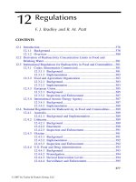
(Figure 12.1). For pesticide monitoring programs, some general guidelines should
Feedback
Analysis
Sampling strategy
Site selection
Identify
possible
sites
Pilot study
Establish management
authorities
Identify the parties
concerned
Define study objectives
Sample
collection

Data analysis
Data interpretation
Communication
Publications
Workshops
Reporting
Planning
Conducting
FIGURE 12.1 Phases in planning, conducting, and reporting of a monitoring program.
(From Calamari, D., et al., Evaluation of Persistence and Long Range Transport of Organic
Chemicals in the Environment, G. Klecka et al., eds., SETAC, 2000.)
ß 2007 by Taylor & Francis Group, LLC.
be taken into consideration including the clear statement of the objectives, the
complete description of the area as well as the locations and frequency of sampling,
and the number of the samples. The geographical limits of the area, the present and
planned water or land uses, and the present and expected pesticide pollution sources
should be identified. Background informat ion of this type is of great help in planning
a representative monitoring program covering all the sources of the spatial and
temporal variability of the pesticide environmental concentration. Appropriate stat-
istical analysis can be used to determine probability distributions that may be used to
select locations for further sampling programs and for risk assessment. The fieldwork
associated with the collection and transp ortation of samples will also account for a
substantial section of the plan of a monitoring program. The development of
meaningful sampling protocols has to be planned carefully taking into account the
actual procedures used in sample collection, handling, and transfer [22]. The design
of a sampling should target the representativeness of the samples that is related to
the number of samples and the selection of sampling stations intended within the
objectives of the study. The sampling process of taking random grab samples and
individually analyzing each sample is very common in environmental monitoring
programs and is the optimal plan when a measurement is needed for every sample.

However, the process of combining separate samples and analyzing this pooled
sample is sometimes beneficial. Such composite sampling process is generally
used under flow conditions and in situations where concentrations vary over time
(surface water or air sampling), when samples taken from varying locations as well
as when representativeness of samples taken from a single site need to be improved
by reducing intersample variance effects. Composite samplin g is also used to
increase the amount of material available for analysis, as well as to reduce the
cost of analysis. However, certain limitations must be taken into account and it
should be used only when the researcher fully understands all aspects of the plan of
choice [18,22].
Apart from sampling, the selection and the performance of the analytical method
used for the determination of pesticides is a very critical subject. Earlier chapters of
this book discuss the various methods that can be successfully applied to monitor
pesticides in various environmental compartments. Another point that should be
considered in the planning stage concerns the quality assurance=quality control
(QA=QC) procedures to produce reliable and reproducible data. These quality issues
relate to the technical aspects of both sampling and analysis. The quality of the data
generated from any monitoring program is defined by two key factors: the integrity
of the sample and the limitations of the analytical methodology. The QA=QC
procedures should be designed to establish intralaboratory controls of sample col-
lection and preparation, instrument operation, and data analysis and should be
subjected to ‘‘ Good Analytical Practices’’ (GAP). Laboratories should participa te
in a series of intercalibration exercises and chemical analysis cross-validations to
avoid false positives [19,23].
As already mentioned, the whole planning of a monitoring program is aimed at
the gene ration of reliable data but it is acknowledged that simply generating good
data is not enough to meet monitoring objectives. The data must be proceeded and
presented in a manner that aids understanding of the spatial and temporal patterns,
ß 2007 by Taylor & Francis Group, LLC.
taking into consideration the characteristics of the study areas, and that allows the

human impact to be understood and the consequences of management action to be
predicted. Thus, different statistical approaches are usually applied to designing,
adjusting, and quantifying the informational value of monitoring data [20]. However,
because data are often collected at multiple locations and time points, correlation
among some, if not all, observations is inevitable, making many of the statistical
methods taught to be applied. Thus, in the last decade geographic information
systems (GIS) and computer graphics are used that have enhanced the ability to
visualize patterns in data collected in time and space [24]. In summary, statistical
methods, including chemometric methods, coupled to GIS are used in recent years to
display the most significant patterns in pesticide pollution [18].
Finally, one of the major parameters of the monitoring plan should be the cost of
the program. A cost estimate should be prepared for the entire program, including
laboratory and field activities. The major cost elements of the monitoring program
include personnel cost; laboratory analysis cost; monitoring equipment costs;
miscellaneous equipment costs; data analysis and reporting costs.
As a conclu sion based on the earlier arguments, monitoring activities must imply
a long-term commitment and can be summarized as follows [18–20]: (1) establish-
ment of monitoring stations for different environmental compartments to fill spatio-
temporal data; (2) intensive monitoring over wider areas, and continuation of
existing time trend series; (3) establishment of standardized sampling and analytical
methods; (4) follow-up of improved quality assuranc e=quality control protocols;
(5) adequate reporting of the results in the more meaningful manner; and (6) estima-
tion of the monitoring program cost.
12.2.2 SELECTION OF PESTICIDES FOR MONITORING
The number and nature of pesticides monitored depended on the objectives of the
monitoring study. Some studies concentrated on a limited number of target pesti-
cides, whereas others performed a broad screening of different compounds. Research
has usually been focused on the most commonly used pesticides either in the
agricultural area around the studied sites or in the country concerned. The selection
of pesticides for monitoring has also been based on pesticide properties (e.g.,

toxicity, persistence, and input), the cost, as well as on special directives and
regulations [25].
The diversity of aims and objectives for the various monitoring programs has
resulted in a variety of active ingredients and metabolites monitored in the studies
performed.
For instance, until the beginning of the 1990s, halogenated, nonpolar pesti-
cides were the focus of interest. As the environmental fate of hydrophobic pesticides
became more generally understood and new, more environmental-friendly, pesticide
products are introduced in the market, there has been an increase in monitoring studies
that focused on currently used pesticides known to be present in the environment.
Whereas environmental concentrations of halogenated, nonpolar pesticide s have
generally declined during the past 20 years, a nd whereas current concentrations in
surface water are below the drinking water standards, concerns nevertheless remain,
ß 2007 by Taylor & Francis Group, LLC.
because these substances persist in the environment and accumulate in the food chain,
thus continue to be in the list for investigation. Current screening strategies have also
included pesticides with endocrine disruption action due to their newly discovered
ecotoxicological problems on human health and environment. Among the most
studied chemical classes of pesticides are the s-triazines, acetamides, substituted
ureas, and phenoxy acids from the group of herbicides and organophosphorus and
carbamates from the group of insecticides. Currently, moder n fungicides have gain
attention since their uses have been increased and new compounds have been intro-
duced in the market.
Although that all new compounds or new uses of existing pesticides are carefully
scrutinized, the list of pesticide of interest for monitoring programs is not getting
shorter and there is a continuing need for development of new criteria that allow the
prediction of which pesticides could be of concern for monitoring.
12.2.3 TYPES OF MONITORING
Pesticides can occur in all compartments of the environment or in other words in
any or all of the solid, liquid, or gaseous phases. The environment is not a simple

system and consequently pesticide monitoring should be carrying out in a specific
phase (e.g., volatile pesticides in air) or may encompass two or more phases and=or
media (e.g., water and sediment in the marine environment). Primary environmental
matrices that are usually sampled for pesticide investigations include water, soil,
sediment, biota, and air. However, each of these primary matrices includes many
different kinds of samples. A brief description of each type of monitoring is given in
the next paragraphs.
12.2.3.1 Air Monitoring
Historically, water contamination has garnered the lion’s share of public attention
regarding the ultimate fate of pesticides. In contrast, atmospheric monitoring is less
expanded since the atmospheric residence time of a pesticide is very variable.
However, in recent years, air quality has become a very important concern as more
and more studies have shown the great impact of atmospheric pesticide pollution on
environment and health. Pesticides can be potential air pollutants that can be c arried
by wind, and deposited through wet or dry deposition processes. They can revol-
atilize repeatedly and, depending on their persistence in the environment can travel
tens, hundreds, or thousands of kilometers [26]. For example, currently used organo-
chlorine pesticides (OCPs) like endosulfans and lindane have been detected in arctic
samples [9,27] where, of course, they have never been used.
The design of monitoring networks for air pollution has been treated in several
different ways. For example, monitoring sites may be located in areas of severest
public health effects, which involves consideration of pesticide concent ration, expos-
ure time, population density, and age distribution. Alternatively, the frequency of
occurrence of specific meteorological conditions and the strength of sources may be
used to maximize moni tor coverage of a region with limited sources.
Air concentrations of pesticides may vary over the scales of hours, days, and
seasons since they respond to air mass direction and depositional events.
ß 2007 by Taylor & Francis Group, LLC.
The sampling methods of pesticides in air may be divided into active (pump or
vacuum-assisted sampling) or passive techniques (passive by diffusion gravity or

other unassisted means). The sampling interval may be integrated over time or it may
be continuous, sequential, or instantaneous (grab sampling). Measurements obtained
from grab sampling give only an indication of what was present at the sampling site
at the time of sampling. However, they can be useful for screening purposes and
provide preliminary data needed for planning subsequent monitoring strategies.
Probably, the collection of pesticides by using passive air samplers (PAS) is the
most common sampling method for air samples. PAS continuously integrate the air
burden of pesticides and give real-time or near-time assessment of the concentration
of pesticide in air [8,22,28]. Most of the passive air sampling measurements have
been performed using semipermeable membrane devices (SPMDs) [28], polyure-
thane foam (PUF) disks [29], and samplers employing XAD-resin [30].
12.2.3.1.1 Occurrence and pesticide levels in air monitoring studies
Numerous investigations around the world consistently find pesticides in air, wet
precipitation, and even fog. Research in the 1960s to 1980s, for example, has found
the infamous pesticide DDT and other OCPs in Antarctic ice, penguin tissues, and
most of the whale species [31]. Monitoring programs have been established in many
countries for the spatial and temporal distribution of persistent OCPs such as DDTs,
HCHs, cyclodienes [19]. While many of the newer, currently used pesticides are less
persistent than their predecessors, they also contaminate the air and can travel many
miles from target areas. Of these, chlorothalonil, chlorpyrifos, metolachlor, terbufos,
and trifluralin have been detected in Arctic environmental samples (air, fog, water,
snow) by Rice and Cherniak [32] and Garbarino et al. [27] or in ecologically
sensitive regions such as the Chesapeake Bay and the Sierra Nevada mountains
[33]. In general, herbicides such as s-triazines (atrazine, simazine, terbuthylazine),
acetanilides (alachlor and metolachlor), phenoxy acids (2,4-D, MCPA, dichloprop)
are among the most frequently looked for and detected in air and precipitation.
Regarding the modern insecticides, organophosphorus compounds (parathion, mala-
thion, diazinon, and chlorpyrifos) have been looked for most often. The occurrence
of other groups of pesticides in air and rain has been generally poorly investiga ted
[34]. Concentrations of modern pesticides in air often range from a few picograms

per cubic meter to many nanograms per cubic meter. In rain, concentrations have
been measured from few nanograms per liter to several micrograms per liter.
However, concentrations in precipitation depended not only on the amount of
pesticides present in the atmosphere, but also on the amounts, intensity, and timing
of rainfall [34]. Concentrations in fog are even higher. Deposition levels are in
the order of several milligrams per hectare per year to a few grams per hectare per
year [9,10].
In general, air monitoring studies have been conducted on an ad hoc basis and
are characterized by a small number of sampling sites, covering limited geographical
areas and time periods. In the United States and Canada [10], however, some large,
nationwide studies have been conducted. In contrast, most European (EU) monitor-
ing studies have been focused on rain rather than in air. So far, at least over 80
pesticides have been detected in precipitation in Europe and 30 in air [35]. However,
ß 2007 by Taylor & Francis Group, LLC.
the lack of consistency in sampling and analytical methodologies holds for both
United States and European studies [7].
An example of characteristic pesticide monitoring programs in air and rainwater
can be mentioned, the Integrated Atmospheric Deposition Network (IADN, Canada),
based on several sampling stations on the Great Lakes [36]. The Canadian Atmos-
pheric Network for Current Used Pesticides (CANCUP, 2003) also provides
new information on currently used pesticides in the Canadian atmosphere and
precipitation [37]. Last example from monitoring of pesticides in rainwater is the
survey established by Flemish Environmental Agency (FE A) in Flanders, Belgium
[38] that monitors >100 pesticides and metabolites at eight different locations.
12.2.3.2 Water Monitoring
The principal reason for monitoring water quality has been, traditionally, the need to
verify whether the observed water quality is suitable for inte nded uses. However,
monitoring has also evolved to determine trends in the quality of the aquatic
environment and how the environment is affected by the release of pesticides and=or
by waste treatment operations. Currently, spot (bottle or grab) sampling, also called

as active sampling, is the most commonly used method for aquatic monitoring of
pesticides. With this approach, no special water sampling system is required and
water samples are usually collected in precleaned amber glass containers. Although
spot sampling is useful, there are drawbacks to this approach in environments where
contaminant concentrations vary over time, and episodic pollution events can be
missed. Moreover, it requires relatively large number of samples to be taken from any
one location over the entire duration of sampling and therefore is time-consuming
and can be very expensive. In order to provide a more representative picture and to
overcome some of these difficulties, either automatic sequential sampling to provide
composite samples over a period of time (24 h) or frequent sampling can be used.
However, the former involves the use of equipment that requires a power supply, and
needs to be deployed in a secure site, and the latter would be expensive because of
transport and labor costs .
In the last two decades, an extensive range of alternative methods that yield
information on environmental concent rations of pesticides have been developed.
Of these, passive sampling methods, which involve the measurement of the concen-
tration of an analyte as a weighted function of the time of sampling, avoid many of the
problems outlined earlier, since they collect the target analyte in situ without affecting
the bulk solution. Passive sampling is less sensitive to accidental extreme variations of
the pesticide concentration, thus giving more adequate information for long-term
monitoring of aqueous systems. Comprehensive reviews on the use of equilibrium
passive sampling methods in aquatic monitoring as well as on the currently avail-
able passive sampling devices have been recently published [39–42]. Despite the well-
established advantages, passive sampling has some limitations such as the effect of
environmental conditions (e.g., temperature, air humidity, and air and water move-
ment) on analyte uptake. Despite such concerns, many users find passive sampling an
attractive alternative to more established sampling procedures. To gain more general
appeal, however, broader regulatory acceptance would probably be required.
ß 2007 by Taylor & Francis Group, LLC.
Other technologies available for water sampling include continuous, online

monitoring systems. In such installations, water is conti nuously drawn from water
input and automatically fed into an analytical instrument (i.e., LC-MS). These
systems provide extensive, valuable information on levels of pesticides over time;
however they require a secure site, are expensive to install, and have a significant
maintenance cost [42].
Finally, another approach available and already in use for monitoring water
quality includes sensors. A wide range of sensors for use in pesticide monitoring
of water have been developed in recent years, and some are commercially available.
These are based on electrochemical or electroanalytical technologies and many are
available as miniaturized screen-printed electrodes [43]. They can be used as field
instruments for spot measurements, or can be incorporated into online monitoring
systems. However, some of these methods do not provide high sensitivity, and in
some case specificity, as they can be affected by the matrix and environmental
conditions, and thus it is necess ary to define closely the conditions of use [44].
12.2.3.2.1 Occurrence and pesticide levels in water samples
The majority of the pesticide monitoring effort goes into monitoring surface fresh-
waters (including rivers, lakes, and reservoirs) and monitoring programs for pesti-
cides in marine waters and groundwaters have received less attention. Within
Europe, the contamination of freshwaters by pesticides follows comparable concen-
tration levels and patterns as recorded in most countries. Among the most commonly
encountered herbicide compounds in European freshwaters were atrazine, simazine,
metolachlor, and alachlor. s-Triazine herbicides are widely applied herbicides in
Europe for pre- and postemergence weed control among various crops as well as
in nonagricultural purposes. In some studies, acetamide herbicides alachlor and
metolachlor (which are also used to control grasses and weeds in a broad range of
crops) were also detected at levels comparable with those of the triazines. Concern-
ing insec ticide concentrations in European freshwaters mainly organophosphates and
organochlorine insecticides have been detected. Diazinon, parathion methyl, mala-
thion, and carbofuran were the most frequently detected compounds [1]. OCPs
continue to be present in freshwaters, but at low levels, due to their high hydro-

phobicity. Among them, lindane was the most frequently detected compound. Other
OCPs include a-endosulfan and aldrin. Fungicides were not generally present at
high concentrations in European surface waters and usually the detected levels were
below detection limits. Only sporadic runoff of certain fungicides (e.g., captafol,
captan, carbendazim, and folpet) was reported in estuaries of major Mediterranean
rivers [45]. Finally, for the United States, the most commonly encountered com-
pounds also include atrazine, simazine, alachlor, and metolachlor from herbicides
and diazinon, malathion, and carbaryl from insecticides [46].
The water monitoring studies around the world have routinely focused on tracing
parent compounds rather than their metabolites. Thus, little data are available on the
occurrence of pesticide transformation products in freshwaters, including mainly
transformation products of high-use herbicides, such as acetamide and triazine
compounds. For example, desethylatrazine, metabolite of atraz ine, has been detected
in rivers of both United States [47] and Europe [48].
ß 2007 by Taylor & Francis Group, LLC.
Agricultural uses result in distinct seasonal patterns in the occurrence of a
number of compounds, parti cularly herbicides, in freshwaters. Regarding rivers,
critical factors for the time elapse between the period of pesticide application in
cultivation and their occurrence in rivers include the characteristics of the catchment
(size, climatological regime, type of soil, or landscape) as well as the chemical and
physical properties of the pesticides [49]. The size of the drainage basin affects the
pesticide concentration profile and Larson and coworkers showed that in large rivers
the integrating effects of the many tributaries result in elevated pesticide con-
centrations that spread out over the summer months. In rivers with relatively small
drainage basins (50,000–150,000 km
2
), pesticide concentrations increased abruptly
and the periods of elevated concentrations were relatively short—about 1 month—as
pesticides were transported in runoff from local spring rains in the relatively small
area [50]. Although for the smaller drainage basins of the Mediterranean area short

periods of increased pesticide concentrations would be expected, more spread out
pesticide concentration pro files are observed. This is probably due to delayed
leaching from soil as a result of dry weather conditions, which is reflected by the
low mean annual discharges [1,51]. Generally, low concentrations were observed
during the winter months because of dilution effects due to high-rainfall events and
the increased degradation of pesticides after their application. Thus, pesticides were
flushed to the surface water systems as pulses in response to late spring and early
summer rainfall as reported elsewhere [52].
The character of the landscape in combination with the type of cultivation in the
catchment area may as well affect the temporal variations in riverine concentrations
of pesticides. For example, for the relatively large basin of the river Rhone, the
concentration of triazines displays a short peak from late April to late June with
relatively constant concentrations during the rest of the year [53], due to the fact that
herbicides are used in vineyards situated on mountain slopes which promotes rapid
runoff. Finally, similar trends and temporal variations were observed also in lakes.
The only difference is that residues were detected during a longer period as a result
of the lower water flushing and renewal time compared with rivers.
Several pesticides and their metabolites have also been identified in groundwater
[54]. However, fewer pesticide measurements are available around the world located
mainly in the area of United States and Europe. In previous published studies that
summarized the groundwater monitoring data for pesticides in the United States [55],
researchers reported that at least 17 pesticides have been detected in groundwater
samples collected from a total of 23 State s. About half of these chemicals were
herbicides such as alachlor, atrazine, bromacil, cyanazine, dinoseb, metolachlor,
metribuzin, and simazine. The reported concentrations of these herbicides ranged
from 0.1 to 700 mg=L. Cohen et al. [55] have compiled the chemodynamic properties
of the detected pesticides in groundwater and concluded that most of these chemicals
had aqueous solubility in excess of 30 mg=L and degradation half-lives longer than
30 days.
In EU countries, as in the case of the United States, commonly used pesticides

such as triazines (atrazine and simazine) and the ureas (diuron and chlortoluron),
which are used in relatively large quantities, are often detected in raw water sources.
Because atrazine and simazine frequently appear in groundwater, several European
ß 2007 by Taylor & Francis Group, LLC.
countries ha ve banned or restrict ed the use of product s containing these active
ingredient s and a recent asses sment reveal ed a stat istically signi fi cant down ward
trend in the contam ination of groundw ater with atrazine and its metaboli tes in a
numbe r of Eur opean countr ies [15]. However , in Baden – Wurttem berg, Germany,
where atraz ine concent rations in groundw ater appear to be decreas ing, concent ra-
tions of another triazine herbicide, hexazi non, show an upward trend [15]. As an
examp le of groundw ater monitor ing progra m, the Pe sticides in European Ground-
waters (P EGASE ) is a detai led study of repres entative aqu ifers. Furthermor e, the
Pesticide Nationa l Synthes is Projec t which is a part of the U.S. Geol ogical Survey ’s
Nationa l Water Qual ity Assessm ent Program (NAWQ A) with the aim of long- term
assessmen t of the status and trend s o f wat er resour ces including pesticide s as o ne o f
the highest priority issues is also a nice examp le for water moni toring progra ms
(http:==ca.water.u sgs.go v=pnsp=).
As ment ioned previ ously, limit ed monitor ing data are avail able for the occu rrence
of pesti cides in mari ne waters. Main ly estua rine envir onmen ts, ports , and marinas
have been moni tored for pesticide loadin gs. Ni ce examp le of such moni toring
progra m is the Fluxes of Agr ochem icals into the Marine Environ ment (FAM E)
project, suppor ted by the Eur opean Union, that provi de informat ion for Rhone
(France) , Ebro (Spain ), Louros (Greece), and Western Scheldt (The Netherla nds)
river=estuary systems [56] and ME DPOL progra m for monitor ing prior ity fungi cides
in estuarine areas of the Medi terranean regio n [44,57 ]. In addition, the Assessment of
Antifo uling Agents in Coastal Environ ment s (ACE) project of the Eur opean Com-
missio n (1999 –2002 ) provi des data concern ing contam ination and effect s=risk s of the
most popula r bioci des c urrently u sed in antifouling paint s to prevent fouli ng of
submerged surfa ces in the sea as alternativ es to tri butyltin compo unds. A number
of booster bioci des have bee n de tected in many Eur opean countries including Irgar ol

1051, diuro n, sea nine, and c hlorothal onil. The occurr ence, fate, and toxi c effects of
antifouli ng bioci des have be en revie wed recently [58,59].
12.2.3. 3 Soil an d Se diment Monit oring
Soil a nd sediment compa rtments might also be regard ed as reservoirs for many types
of pesticide s. Althoug h high amoun ts of pesticide as well as a c omplex patte rn of
their met abolites are usually presen t in soils, this mat rix is not generally moni tored
on a regul ar basis and there is a g ap in knowledge on n ational and global level
regard ing the pesticide resi due levels. The majo rity of the investig ation studies were
carried out by resear chers ’ initiative or licensing of new subst ances or under the
frame of founded p rojects. Reg ardin g Eur ope, recent discu ssions have taken place to
conside r regul ation of persi stence o f soil residues beyond the guidelines given in the
Directive 91=414=EEC [17]. In this regard, stro nger e mphasis should be given to soil
monitor ing progra ms such a s Moni toring the State of European Soils (MO SES;
http:==projects- 2004.j rc.cec.eu .int=) and Env ironment al Indicators for Sustaina ble
Agricul ture (ELIS A; http:==www.ecnc.nl=CompletedPr oject s=Elisa _119.ht ml).
In contrast to soils, sediments are usually monitored for pesticide contamination.
Sediments from river, lake, and seawaters provide habitat for many benthic and
epibenthic organisms and are a significant element of aquatic ecosys tems. Many
ß 2007 by Taylor & Francis Group, LLC.
pesticide compounds, because of their h ydrophobic nature, such as OCPs, are known
to associate strongly with natural sediments and dissolved organic matter and high
concentrations of pesticides are frequently found in bed sediments, both freshwater
and coastal [60]. Monitoring studies using sediment core stratification also have the
advantage of providing information on the chronologies of accumulation rates of
persistent pesticides. This information is important to evaluate the rate of emission
from probable sources, and to relate specific rates of pesticide accumulation and rates
of ecosystem response. Sedime nt monitoring is also a task for the correct implemen-
tation of the Water Framework Directive (WFD) to assess any changes in the status
of water bodies.
Soils and sediments are typically very inhomogeneous media, thus a large

number of samples may be required to characterize a relatively small area. Sampling
sites could be distributed spatially at points of impact, reference sites, areas of future
expected changes, or other areas of particular interest. Selection of specific locations
is a subject of accessibility, hydraulic conditions, or other criteria. The devices used
for soil and sediment sampling are usually grab samplers or corers. Grab samplers
are available for operation at surfacial depths. Box corers or multicorers can be
employed if more data on the chronologies of accumulation rates of the analytes are
needed.
12.2.3.3.1 Occurrence and pesticide levels in soils and sediments
In view of the current concern about the assessment of soil quality, some recent
pesticide monitoring studies have been conducted within Europe [11,12,61,62].
According to the results a variety of pesticides, mainly herbicides and insecticides
appeared consistently as contaminants of the tested soil samples. Concerning pesti-
cide contamination of soils in United States pesticides such as atrazine, chlorpyrifos,
and others have been detected [63].
The monitoring studies performed on sediments show a large number of detected
pesticides over the last 40 years. Most of the target analytes detected were OCPs and
their transformation products despite the fact that most of them were banned or
severely restricted by the mid-1970s in the United States and EU. This reflects both
the environmental persistence of these compounds and limited targe t analytes list.
DDT and metabolites, chlordane compounds, a-, b-, g-HCH, and dieldrin were the
most detected pesticides in bed sediments. Other OCPs that sometimes were detect ed
included endosulfan compounds, endrin and its metabolites, heptachlor and hepta-
chlor epoxide, methoxychlor, and toxaphene [64].
Recent studies in sediment cores have shown that concentration levels of OCPs
have a relative steady state for DDTs, with a slight decrease in the top layers,
suggesting a slight decline in their concentrations due to restrictions in their usage
[65]. Besides the OCPs, a few compounds in other pesticide classes were detected in
some studies. Most of these pesticides contained chlorine or fluorine substituents
and have medium hydrophobicity. Currently used pesticides detected in sediments

included the herbicides atrazine, ametryne, prometryne, trifluralin, dicamba, ala-
chlor, metholachlor, and diuron; the organophosphorus insecticides diazinon, chlor-
pyrifos, ethion, and pyrethrines such as cypermethrin, fenverate, and deltamethrin
[2,3]. Of pesticides from other chemical classes, most were targeted at relatively few
ß 2007 by Taylor & Francis Group, LLC.
sites. Examples in this case include the booster biocides such as irgarol, diuron, and
chlorothalonil, which were detected in coastal marine sediments [58,59].
12.2.3.4 Biological Monitoring
A lot of b iological organisms, from flora and fauna to human beings, are monitored
to determine amounts of these pesticides that are present in the environment and
evaluate the associated hazard and risk. This type of monitoring is an essential part of
pesticide pollution studies that is known as biological monitoring or biomonitoring.
Another important facet of environmental biomonitoring is the emerging field
of environmental specimen banking. A specimen bank acts as a bridge connecting
real-time monitoring with future trends monitoring acti vities.
In general, biomonitoring overcomes the problem of achieving a snapshot of the
quality of the environment, and can provide a more representative picture of average
conditions over a period of weeks to months. However, the use of biomonitors
has limitations since some compounds are metabolized or eliminated at a rate close
to the rate of uptake, and thus are not accumulated. Moreover, because of cost, the
monitoring may be carried out only on a limited number of species and there is no
guarantee that important species will be selected. Not all pesticides are amenable
to biological monitoring. Pesticides that are rapidly absorbed and are neither seques-
tered nor metabolized to a significant extent are usually good candidates. Pesticides
that have a high tendency to bioaccumulate, such as OCPs, are the most commonly
detected pesticides in biota samples.
Sample collection methods must be selected considering both the organisms to be
collected and the conditions that will be encountered. Organisms that can be deployed
for extended periods of time, during which they passively bioaccumulate pesticides in
the surrounding environment are usually selected. Plankton, bacteria, periphyton,

benthos, fish, and fish-eating birds are the most common specimens for monitoring
aquatic compartment. Analysi s of the tissues or lipids of the test organism(s) can give
an indication of the equilibrium level of waterborne pesticide contamination. Adipose
tissues, eggs, and liver have been recognized as accumulators of lipophilic pesticides
and they are usually monitored to quantify the threat of pesticide contamination in
species of wildlife. Apart from aquatic organisms and wildlife species, increasing
attention is focused on the monitoring and assessment of human exposure to pesticides
throughout the world. Urine, blood, and exhaled air are the mostly used specimens for
routine biological monitoring to human beings. Other biological media include
adipose tissue, liver, saliva, hair, placenta, and body involuntary emissions such as
nasal accretions, breast milk, and semen. However, many of these media have some
serious problems (e.g., matrix effects, insufficient dose–effect relationships) and
they do not necessarily provide consistent results to that from blood, urine, or
breathe [66].
12.2.3.4.1 Occurrence and pesticide levels in biota
Several studies have been conducted around the world on the general topic of
biological monitoring of pesticides. As in the case of sediments, most of the studies
reveal the presence of OCPs and their transformation products. These compounds
have been detected in different human specimens such as human milk, saliva, urine,
ß 2007 by Taylor & Francis Group, LLC.
adipose tissues, and liver [66–69]. DDT and its metabolites are still the most
frequently determined compounds, especially in samples from developing countries.
Other OCPs determined were cyclodienes such as diel drin, aldrin, endrin, heptachlor
and its epoxide, chlordane as well as isomers of hexachlorocyclohexane [67].
Moreover, endosulfan I and II and the sulfate metabolite have been detected in fatty
and nonfatty tissues and fluids from women of reproductive age and children
in Southern Spain [69]. Apart from OCPs, currently used pesticides have also
been detected in different human biological samples. Examples include bromophos
in blood; fenvalerate, malathion, terbufos, and chlorpyrifos methyl in urine; paraqua t,
2,4-D, and pentachlorophenol in urine and blood; carbaryl, atrazine, and ethion in

saliva; and DDT in blood and adipose tissue, and so on [68]. From the currently used
pesticides, organophosphorus pesticides (OPPs) are the most frequently detect ed in
different human biological fluids. Apart from the parent compo unds, the measurement
of dialkyl phosphate metabolites has been frequently used to study exposure to a wide
range of OPPs. These metabolites have been detected in urine samples from exposed
workers as well as from people who had no occupational exposure to OPPs. In
addition, metabolites of carbamates (carbaryl, carbofuran) and pyrethrines (cyperme-
thrin, deltamethrin, permethrin) have been also detected in urine samples [66–68].
Except of human biological samples, the accumulation pattern of OCPs in aquatic
organisms as well as terrestrial wildlife has been reported. For example, concentration
levels of DDT and its metabolites have been detected in different species of arctic
wildlife such as terrestrial animals, fish, seabirds, and marine mammals [70]. Exten-
sive results have also reported for various bird species [4,71,72], fish, and amphibian
[73,74] as well as mammals [75,76], when adipose tissues, liver, or eggs of these
organisms have been analyzed. p,p
0
-DDE, a major metabolite of DDT, continued to be
the dominating OCP burden in almost all the tested species, whereas cyclodienes and
HCHs occurred at lower concentrations. Apart from OCPs, several currently used
pesticides (despite their lower bioaccumulation) such as trifluralin, chlorothalonil,
parathion methyl, phosalone, disulfoton, diazinon, dimethoate, and chlorpyrifos have
also been detected in biota samples [6,77]. It is notable that a high variability in the
concentrations of pesticides within the same species was observed and this was related
to sampling location, age, and sex and with condition and stage of the life cycle
(starvation=feeding, lactation, illness=disease) of the analyzed organisms.
A comparison of studies regarding the aquatic monitoring in sediments and biota
suggests that pesticides were detected more often in aquatic biota than in bed
sediment. In addition, the transformation products were also found at higher levels
in biota samples than in associated sediment [4].
An example of monitoring program that report a range of diverse invertebrate,

vertebrate, and human relevant tests is the Comparative Research on Endocrine
Disrupters—Phyloge netic Approach and Common Principles focusing on Andro-
genic=Antiandrogenic Compounds (COMPRENDO) project [78].
12.2.4 WATER FRAMEWORK DIRECTIVE AND MONITORING STRATEGIES
The potential adverse consequences that are derived from the use of pesticides
have led to the development of special regulations. For instance, in the European
ß 2007 by Taylor & Francis Group, LLC.
Community, several directives and regulations have been issued with the aim of
safeguarding human health and the environment from the undesirable effects
of these chemicals (i.e., Dangerous Substances (76=464=EC) [79], Groundwater
(80=68=EEC) [80], and Pesticide (91=414=EEC) [17] Directives). The newly intro-
duced WFD (2000=60=EC) [81] is widely recognized as one of the most ambitious
and comprehensive pieces of European environmental legislation. Its aim is to
improve, protect, and prevent further deterioration of water quality at the river-
basin level across Europe. The term ‘‘water’’ within the WFD encompasses most
types of water bodies. Furthermore, to monitor the progressive reduction in contam-
inants, trend studies, whether spatial or geographical, should be envisaged through
the measurement of contaminants in sediment and biota. The Directive aims to
achieve and ensure ‘‘good quality’’ status of all water bodies throughout Europe by
2015, and this is to be achieved by implementing management plans at the river-
basin level. The WFD foresees that water quality should be monitored on a system-
atic and comparable basis. Thus, technical specifications should follow a common
approach (e.g., the standardization of monitoring, sampling, and methods of
analysis). Chemical monitoring is expected to be intensified and will follow a list
of 33 priority chemicals (inorganic and organic pollutants including pesticides) that
will be reviewed every 4 years. The concentrations of the priority substances in
water, sediment, or biota must be below the Environmental Quality Standards
(EQSs) and this is expressed as ‘‘compliance checking.’’ However, EQSs for these
substances including pesticides have yet to be stated [25,82]. The derivation of EQSs
through a risk assessment procedure is presented later in this chapter.

The implementation of the WFD is based on a three-level monitoring system,
which will form part of the management plans and was to be implemented from
December 2006 [81,83]: This include (1) surveillance monitoring aimed at assessing
long-term changes in natural conditions; (2) operational monitoring aimed at pro-
viding data on water bodies at risk or failing environmental objectives of the WFD;
and (3) investigative monitoring aimed at assessing the causes of such failure and
the effects.
Comprehensive reviews focused on principal monitoring requirements of the
WFD as well as on emerging techniques and methods for water quality monitoring
have been published recently to identify and outline the tool s or techniques that may
be considered for water quality monitoring programs necessary for the implementa-
tion of WFD [24,83].
12.3 ENVIRONMENTAL EXPOSURE AND RISK ASSESSMENT
12.3.1 E
NVIRONMENTAL EXPOSURE
12.3.1.1 Point and Nonpoint Source Pesticide Pollution
Environmental exposure of pesticides can be occurred by point and nonp oint
sources. A point source can be any single identifiable source of pollution from
which pesticides are discharged such as the effluent pipes, careless storage, and
disposal of pesticide containers, accidental spills, and overspray. Pesticide move-
ment away from the targeted application site is defined as nonpoint source pollution
ß 2007 by Taylor & Francis Group, LLC.
and can occur through runoff, leaching, and drift. Nonpoint source pollution occurs
over broad geographical scales and because of its diffuse nature it typically
yields relatively uniform environmental concentrations of pesticides in surface
waters, sediments, and groundwater. Runoff is the surface movement of pesticide
in water or bound to soil particles, while leaching is the downward movement of a
pesticide through the soil by water percolation. Drift is the off-target movement
by wind or air currents and can be in the form of spray droplet drift, vapor drift, or
particle (dust) drif t.

12.3.1.2 Environmental Parameters Affecting Exposure
The environmental parameters that affect pesticide exposure could be classified as
follows:
1. Soil characteristics and field topography: Texture composition and pH are
the main soil properties that affect pesticide fate and transport, whereas
topographic characteristics of the fields like watershed size, slope, drainage
pattern, permeability of soil layers affect greatly the potential to generate
runoff water or leachates.
2. Weather and climate: Climatic factors such as the amount and timing of
rainfall, duration, and intensity, as well as temperature and air movement
influence the degree to which pesticides are mobilized by runoff, leaching,
and drift. In addition, temperature and sunlight affect all abiot ic and biotic
transformation reactions of pesticides [84,85].
12.3.1.3 Pesticide Parameters Affecting Exposure
The pesticide factors affecting exposure could be organized on three main sets:
1. Application factors: These include the application site (crop or soil surface)
and method, the type of use (agricultural, nonagricultural applications,
indoor pest management, etc.), the formulation (e.g., granules or suspended
powder or liquid) and the application amount, and frequency. In addition,
the application time does affect its possible routes of transport in the
environment.
2. Partitioning and mobility of pesticides in the environment: The main
physicochemical properties of pesticides that affect their mobility are the
water solubility, vapor pressure, and soil–water partition coefficient (K
oc
).
K
oc
defines the potential for the pesticide to bind to soil particles. Off-target
movement by drift also depends on the spray droplet size and the viscosity

of the liquid pesticide while plant uptake from the soil is another imp ortant
pathway in determining the ultimate fate of pesticide residues in the soil
[84,85].
3. Persistence in the environmental compartments: Persistence is usually
expressed in terms of half-life that is the time required for one-half of
the pesticide to decompose to products other than the parent compound.
The longer a pesticide persists within the environment, the greater the risk it
ß 2007 by Taylor & Francis Group, LLC.
poses to it. Hydrolysis, direct and indirect photolysis, and biodegradation
are the principal pesticide degradation processes and their rates depend on
pesticide chemistry, as well as on environmental conditions [84].
12.3.1.4 Modeling of Environmental Exposure
Monitoring data and environmental modeling are interconnected to each other.
Monitoring could provide the correct input data to models for calibration and
validation or could be devoted to collect data on the timing and magnitude of
loadings. Mathematical models that simulate the fate of pesticides in the environment
are used for developing Environmental Estimated Concentrations (EECs) or Pre-
dicted Environmental Concentrations (PECs). This means ‘‘predicting exposure’’ in
space and time, drawing on available environmental fate data, physicochemical data,
and the proposed agricultural practices and usage pattern associated with the pesti-
cide [86]. A complete presentation of environmental models describing the exposure
of pesticide in the environment is outside the scope of the present chapter. Thus, only
common environmental models that are used to estimate environmental exposure
concentrations for aquatic systems in the context of current risk assessing techniques
will be presented.
The Generic Estimated Environmental Concentration (GENEEC) model, devel-
oped by the EPA, determines generic EEC for aquatic environments under worst-
case conditions (i.e., application on a highly erosive slope with heavy rainfall
occurred just after the pesticide application, the treatment of the entire area—
essentially 10 acres of surface area with u niform slope—with the pesticide, and the

assumption that all runoff drains directly into a single pond). The model uses
environmental fate parameters derived from laboratory studies under standard pro-
cedures as well as soil and weather parameters. The outputs of the model are the
pesticide runoff and environmental concentration estimates [87]. This model can be
used as first tier approach since it is based on a single event and a high-exposure
scenario. On a higher tier approach (second and third), models that can account for
multiple weather conditions and=or multiple sites are used. Such models are the
Pesticide Root Zone Model (PRZM), edge of field runoff=leaching the Exposure
Analysis Modeling System (EXAMS), fate in surface water, and AgDrift (spray
drift) [87] that used additional parameters, more descriptive of the site studied.
PRZM simulates the leaching, runoff, and erosion from an agricultural field and
EXAMS simulates the fate in a receiving water body. The water body simulated is a
static pond, adjacent to the crop of interest. Typical conditions of the site including
the soil characteristics, hydrology, crop management practices, and weather infor-
mation are used. The output of this higher tier analysis is to define the EEC that can
be reasonably expected under variable site and weather conditions. The model yields
an output of annual maxima distributions of peak, 96 h, 21 days, 60 days, 90 days,
and yearly intervals. AgDrift includes generic data for screening level assess-
ments including pesticide formulation, drop height, droplet size, nozzle type, and
wind speed. The earlier approaches are used by pesticide registrants to address
environmental exposure concerns and are frequently combined with geographical
information systems (GIS) to produce regional maps.
ß 2007 by Taylor & Francis Group, LLC.
The fugacity ap proach has a lso proven particula rly suit ed for descri bing the
beh avior of pesticide s in the envir onment. A tier ed system of fugaci ty models has
bee n introduc ed which distingu ishes four level s of complexit y, depend ing on
whet her the system is close d or in exchange with the surro unding environmen t.
The four levels are Level I, close syst em equil ibrium; Level II, equil ibrium stead y
stat e; Lev el III, None quilibri um stead y state; and Lev el IV, None quilibrium non-
stead y state. Levels I and II are used in lower tier approac hes, wher eas Lev el III is

wi dely used in higher tiers to obtai n exposur e concent rations due to emissi on flux
into a prede fined standard envir onmen t. A detailed introduct ion into fugacity-b ased
model ing can be found in Ref. [88].
For evalua ting the impact of manag ement pract ices on potent ial pesti cide leach-
ing, the Groundw ater Loa ding Effects of Agricul tural Manage ment Systems
(GLE AMS) is a widely used, field-scale model . GLE AMS assumes that a field has
ho mogeneous land use, soils, and precipita tion. It consi sts of four major compo n-
ents: hydrology, erosi on, pesticide transport , and nutrients . GLE AMS estimat es
leachi ng, surfa ce runoff , and sediment loss es from the field and can be used as a
tool for compa rative analys is of complex pesticide chemistr y, soil properties , and
clim ate. The model output data are daily, mont hly, a nnual pesti cide mass and
con centratio ns in runoff and sediment .
Finally, a fourth tier approac h can be used ba sed on watershe d site asses sments.
The se asses sments are very compl ex since the lands cape studi ed has a very high
surfa ce area, high diversit y of soils and weather condit ions, varied p roximities of
agric ultu ral lands to receiving wat ers and vario us wat er bodies . Thus, GIS are
comm only used to dist inguish high- risk versus low-ri sk areas on a watershe d
basis . Finally, model ing and monitor ing are often combi ned wi thin tier 4 to provi de
more accurate distrib utio n of pesticide exposur e.
12.3.2 R ISK A SSESSMENT
In order to evalua te the negative impa ct of pesticide s on ecosys tems, the envir on-
mental risk assessment is necessary. It is known that the environmental impact of a
pesticide depends on the degree of exposure and its toxicological properties [89].
The risk assessment procedure involves three main steps: a formulation of the
problem to be addressed followed by an appraisal of toxicity and exposure and
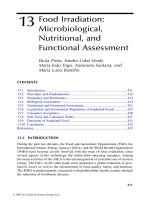
concluding with the characterization of risk. A typical framework for ecological risk
asses smen t is show n in Figure 12.2 [90]. The object ive of the exposur e asses sment is
to describe exposure in terms of source, intensity, spatial and temporal distribution,
evaluating secondary stressors (metabolites) to derive exposure profiles. Usually
exposure assessment involves the measured environmental concentrations (MECs)

derived from monitoring studies or the developing and application of models as
discussed previously.
The toxicity assessment identifies concentrations that when administered to
surrogate organisms result in a measurable adverse biological response. Toxico-
logical assessment is commonly based on laboratory studies with the aim of deter-
mination of the relationship between magnitude of exposure and extent of observed
effects commonly referred as dose–response relationship. Toxicity impacts were
ß 2007 by Taylor & Francis Group, LLC.
usually studied by indicator species selected to represent various trophic levels
within an ecosystem. Representative groups of organisms are assessed for risk to
pesticides, including fish, aquatic invertebrates, algae, and plants from the aquatic
environment and birds, mammals, bees and beneficial arthropods, earthworms, soil
microorganisms, and nontarget plants from the terrestrial environment. All these
organisms are assessed in Europe under 91=414=EEC [17], whereas the USE PA
concentrates on birds and mammals, bees, nontarget plants, and aquatic organisms. It
is impossible and inadvisable to test every species (abunda nt, threatened, endan-
gered) with every pesticide but the need for more toxicological data is acknow-
ledged. Chosen organisms like Daphnia sp. for freshwater zooplankton or rainbow
trout for freshwater fish categories should typically satisfy some basic criteria like the
ecological significance, the abundance and the wide distrib ution, the susceptibility to
pesticide exposure, and the availability for laboratory testing.
Stressor–response analysis can be derived from point estimates of an effect
(i.e., lethal concentration or effect concentration for 50% of the organism population,
LC
50
or EC
50
) or from multiple-point estimates (hazardous concentration for 5% of
the species, HC
5

) that can be displayed as cumulative distribution functions (species
sensitivity distributions, SSDs). In addition, the establishment of cause–effect rela-
tionships from observatio nal evidences or experimental data could be performed.
In a third phase, the risk characterization takes place defining the relationship
between exposure and toxicity. Two different approaches are usually applied for this
Planning
(risk assessor/
risk manager)
Ecological risk assessment
Problem formulation
Risk characterization
Phase 1Phase 2
Analysis
Acquire data, verify, monitor results
Phase 3
Risk management
Discussion between the risk assessor
and risk manager
Characterization
of
ecological effects
Characterization
of
exposure
FIGURE 12.2 EPA framework for ecological risk assessment. (From USEPA, U.S. Environ-
mental Protection Agency, Framework for Ecological Risk Assessment, Risk Assessment
Forum, Washington, D.C., 1992.)
ß 2007 by Taylor & Francis Group, LLC.
purpose. The first is a determinist ic approach that is based on simple exposure and
toxicity ratios and the second is a probabilistic approach in which the risk is

expressed as the degree of overlap between the exposure and effects. Apart from
these methods, numerous Pesticide Risk Indicators (PRIs) based on classification
systems have been developed for fast preliminary assessments and comparative
purposes. All methods will be analyzed in detail later.
The last step in the assessment of risk is the weight-of-evidence analysis.
Strengths, limitations, and uncertainties as well as magnitude, frequency, and spatial
and temporal patterns of previously identified adverse effects and exposure concen-
trations are discussed in the weight-of-evidence analysis.
The assessment of the pesticides risk usually follows a tiered approach adopt.
Tiers are normally designed such that the lower tiers are more conservative, whereas
the higher tiers are more realistic with assumptions more closely approaching reality.
Tier 1 is essentially a screen, thereby to identify low-risk uses, or those groups of
organisms at low risk [91–94]. Higher tier approaches aim to the refinement of risk,
that is, a procedure (method, investigation, evaluation) performed to characterize in
more depth the pesticide risks arising from the preliminary (tier 1) risk assessment.
The risk refinement is triggered to increase more realistic and=or comprehensive sets
of data, assumption and models, and=or mitigation options. Thus, if the assessment
fails to ‘‘pass’’ tier 1, then a more detailed risk assessment is required.
12.3.2.1 Preliminary Risk Assessment–Pesticide Risk
Indicators–Classification Systems
A preliminary estimation of the environmental impact of pesticides use could be
performed through the development and use of PRIs, which are indices that co mbine
the hazard and exposure characteristics for one or several environmental compart-
ments that are assessed separately. PRIs make use of the physicochemical and
biological properties of pesticides and have been used over the years by a large
number of organizations for the purposes of selecting pesticide compounds for
further regulatory a ctions.
Firstly, the development of a PRI is generally based on the concept of risk ratios,
that is, the division of exposure concentration by effect concentration. Several
approaches are based on this standard framework for risk assessment (analyzed in

the following section) such as the Evaluation System for Pesticides (ESPE) [95], the
Ecological Relative Risk (EcoRR) [96], the Environmental Yardstick [97], and
SYNOPS [98]. Although the risk ratio approach is favored by many researchers,
different methodologies have also been used such as the scoring and rankin g of
pesticides in terms of their environmental hazard. In general, the proposed systems
are also based on factors describing the physicochemical and ecotoxicological
properties of pesticides. Such indices are developed by assigning scores to the
previously mentioned properties. The scores are then aggregated using different
algorithms or weights of evidence finally to obtain a numerical or descriptive
index useful for comparati ve assessment of the environ mental impact of pesticide
applications [99]. There are several screening tools in use that were developed for
priority setting in risk assessment, whi ch involves ordering chemicals by scoring and
ß 2007 by Taylor & Francis Group, LLC.
ranking them individually or placing them in group based on degree of concern (e.g.,
high, medium, low). Examples of such approaches are the Scoring and Ranking
Assessment Model (SCRAM), [100], the Environmental Impact Quotient (EIQ)
[101], and the Pesticide Environmental Risk Indicator (PERI) [102]. Such
approaches can be useful for several management purposes such as the selection of
pesticides with less envir onmental impact and the setting of priority list for planning
environmental monitoring or further experimental research [103]. These methods are
simple and fast for ecological screening assessments but are highly arbitrary [104]. In
addition, some other systems use the risk ratio methodologies combined with rating
and scoring approaches in aggregated indices. The short-term or long-term pesticide
risk indexes for the surface water system (PRISW-1, PRISW-2) [104] belong to
this category. Finally, van der Werf and Zimmer [105], in 1998, have developed an
expert system using fuzzy logic (I-pest) to assess the environmental impact of a
single pesticide application to rank various alternatives.
Recently, an attempt to evaluate and compare the v arious methodologies has
been made in Europe by the Concerted Action on Pesticide Environmental Risk
Indicators (CAPER) project [102]. According to the project conclusions, PRIs

differed considerably with regard to several aspects such as purposes, methodolo-
gies, compartments, and effects to take into account. However, the earlier aspects
barely influenced the rankings of the pesticide s. Further details on all the previous
and other approaches and systems are well described and compared in recently
published articles and reports [102,103,105,106]. In conclusion, the present indica-
tors leave room for users and scientists to select the most appropriate indicator,
according to the considered environmental effects and the environmental specific
conditions at national or regional level. However, a harmonized scientific framework
is highly recommended.
12.3.2.2 Risk Quotient–Toxicity Exposure Ratio Method
(Deterministic-Tier 1)
At present, the usual approaches to decide the acceptability of environmental risks
are generally based on the concept of risk ratios expressed as the toxicity–exposure
ratio (TER) adopted by the EU (Equation 12.1) [17] or the risk quotient (RQ)
adopted by USEPA (Equation 12.2) [107]. This methodology usually involves
comparing an estimate of toxicity, derived from a standard laboratory test with a
worst-case estimate of exposure, EEC, or PEC from model applications or peak
measured concentrations, for the US and EU, respectively.
TER ¼
toxicity
exposure
, (12:1)
RQ ¼
exposure
toxicity
: (12:2)
Since the term risk implies an element of likelihood which is usually reported as
probabilities, it is more correct that the risk quotient should be better expressed
as hazard quotient (HQ). However, both terms are used in several studies with the
ß 2007 by Taylor & Francis Group, LLC.

same meaning. Examples of toxicity measurements used in the calculation of RQs
are LC
50
(fish and amphibians, birds); LD
50
(birds and mammals); EC
50
(aquatic
plants and invertebrates); EC
25
(terrestrial plants); EC
05
or nonobserved effect
concentration (NOE C) (endangered plants).
According to Directive 414=91=EEC [17], one standard procedure for the risk
assessment in aquatic systems is the determination of RQ method for three taxo-
nomic groups (i.e., algae, zooplankton, fish) at two effect levels (i.e., acute level,
using LC
50
or EC
50
values and chronic level, using NOEC or predicted noneffect
concentration [PNEC] values).
For assessing the risk in sediments, if results from whole-sediment tests with
benthic organisms are available, the PNEC
sed
has to be derived from these tests.
In the case that not enough reliable ecotoxicological data for sediment-dwelling
organisms are known, the equilibrium partitioning method can be used [108] to
derive PNEC

sed
according to the following equation:
PNEC
sed
¼
PNEC
wat
 K
susp-water
RHO
susp
 1000, (12:3)
where
PNEC
wat
is the PNEC calculated for the water compartment
K
susp–water
is the sediment=water partition coefficient
RHO
susp
is the bulk density of the sediment
The same methodology can be applied for deriving PNEC values for soil using the
corresponding K
psoil
(soil=water) partition coefficient.
For terrestrial systems, the estimat e of the distribution of exposure is separated
into the chemical=physical and biological components. The first component of dose
estimate is the environmental and chemical variables that influence the distribution
of residue levels. The major variables that influence the biological component are

species-dependent including (1) food, water, and soil ingestion rates; (2) dermal and
inhalation rates; (3) dietary diversity; (4) habitat requirements and spatial movement;
and (5) direct ingestion rates. These variables are combined into Equation 12.4 to
estimate the distribution of total dose:
Dose
total
¼ Dose
oral
þ Dose
dermal
þ Dose
inhal
: (12:4)
The oral dose can be further analyzed as follows:
Dose
oral
¼ Dose
food
þ Dose
water
þ Dose
soil
þ Dose
preening
þ Dose
granular
: (12:5)
For each of these sources of oral exposure, the equations which can be used
to esti mate the dose are reported elsewhere [109]. Frequently for birds and mammals,
it is assumed that exposure is through eating treated food items and resi due

concentrations (w=w) in milligram per kilogram are compared with dietary
LC
50
, NOEC.
ß 2007 by Taylor & Francis Group, LLC.
12.3.2.2.1 The use of assessment factors for the characterization
of uncertainty
For many substances, the available toxicity data that can be used to predict eco-
system effects are very limited, and thus, empirically derived assessmen t factors
must be used depending on the confidence with which a PNEC can be derived from
the existing data. The proposed assessment factors according to EC guidelines [108]
are presented in Table 12.1 for water and sediment.
If the database on SSDs from long-term tests for different taxonomic groups
is sufficient, statistical extrapolation methods may be used to derive a PNEC.
In such methods, the long-term toxicity data are log-transformed and fitted according
to the distribution function and a prescribed percentile of that distribution is used
as criterion. Kooijman [110] and Van Straalen and Denneman [111] assume a log-
logistic function, Wagner and Lokke [112] a log-normal function, and Newton
et al. [113] a Gompertz distribution. Newman et al. [113] proposed to bootstrap
the data as a nonparametric alternative whereas Van der Hoeven [114] proposed a
nonparametric method to estimate HC
5
without any assumption about the distri-
bution and without bootstrapping. Aldenberg and Jaworska [115] refined the way to
estimate the uncertainty of the 95th percentile by introducing confidence levels.
The 95% confidence level provides more strict values while 50% of confidence level
is usually applied. According to the earlier discussions, a PNEC value can be
calculated as
TABLE 12.1
Assessment Factors to Derive a PNEC

aquatic
Available Data Assessment Factor
At least one short-term L(E)C
50
from each of three trophic
levels of the base set (fish, Daphnia, and algae)
1000
a
One long-term NOEC (either fish or Daphnia) 100
b
Two long-term NOECs from species representing two trophic levels
(fish, Daphnia, and=or algae)
50
b
Long-term NOECs from at least three species (fish, Daphnia, and algae)
representing three trophic levels
10
b
Species sensitivity distribution (SSD) method 5–1
Field data or model ecosystems Reviewed on case
by case basis
Source: From European Commission, Technical Guidance Document on Risk Assessment in Support of
Council Directive 93=67=EEC for New Notified Substances and Commission Regulation
1488=94 on Risk Assessment for Existing Substances and Directive 98=8=EC of the European
Parliament and the Council Concerning the Placing of Biocidal Products of the Market, EU,
JRC, Brussels, Belgium, 2002.
a
A factor of 100 could be used for pesticides subjected to intermittent release.
b
The same assessment factors are used for derivation of PNEC in sediments using appropriate species.

ß 2007 by Taylor & Francis Group, LLC.
PNEC ¼
5%SSD( 50 % c : i: )
AF
: (12:6)
AF is a n appropr iate assessmen t facto r between 5 and 1 (as propos ed in Tab le 12.1),
reflecting the further uncertainties identified. Confidence can be associated with a
PNEC derived by statistical extrapolation if the database contains at least 10 NOECs
(preferably >15) for different species covering at least 8 taxonomic groups [108].
Uncertainty arises from an incomplete knowledge of the system that is assessed
and it is associated with the following aspects: measurement errors (accuracy),
inherent variability, model error both conceptual and mathematical, assumption
errors, and lack of data. As already mentioned, the characterization of risk at a first
level of assessment is typically highly conservative, both from exposure and effects
characterization perspective and thus it is characterized by high uncertainty. This
means that even values of RQ that are below 1 are quite likely to be capable of
causing an effect. Usually, a safety factor is applied to risk quotients for covering
uncertainty. The factor can vary between 1 and 100, depending on the organisms that
is assessed and whether the toxicity end point is acute, based on short-term effects
(LD=LC=EC
50
) or chronic, based on NOEC [56,94].
Therefore, as a final step in risk characterization procedure, the results of the RQ
are compared with acceptable levels designed by particular jurisdiction [116]. These
regulatory triggers used to categorize the potential risk are defined as levels of
concern (LOC). An example of LOCs of RQ values that can be used for terrestrial
and aquatic risk assessments is shown in Table 12.2. In the EU, TERs for
terrestrial acute effects must be 10 and for aquatic short-term effects 100.
TABLE 12.2
EPA Established Risk Quotients and Levels of Concern for Different

Environmental Appl ications
End Point and Scenario Risk Quotient Nonendangered Endangered
Mammalian acute (granular) EEC=LD50=FT
2
0.5 0.1
Mammalian acute (spray) EEC=LC
50
0.5 0.1
Mammalian chronic (spray) EEC=NOEC 1.0 1.0
Avian acute (granular) EEC=LD50=FT
2
0.5 0.1
Avian dietary (spray) EEC=LC
50
0.5 0.1
Avian chronic (spray) EEC=NOEC 1.0 1.0
Aquatic acute EEC=LC
50
0.5 0.05
EEC=EC
50
Aquatic chronic EEC=NOEC 1.0 1.0
Terrestrial plants EEC=EC
25
1.0 1.0
Aquatic plants EEC=EC
50
1.0 1.0
Source: From Whitford, F. in The Complete Book of Pesticide Management. Science, Regulation,
Stewardship and Communication, John Wiley & Sons, New York, USA, 2002.

ß 2007 by Taylor & Francis Group, LLC.
Chronic and subchr onic TERs 5 and 10 for terr estrial and aquatic speci es, respec t-
ively, are accepta ble.
Descript ive uncert ainty a nalysis is usual ly perfor med in the lower tiered
risk asses sments while sensiti vity analys is and more compl ex model (i.e., Monte
Carlo) simulat ion are usual ly completed in higher tier asses sments. Mont e Car lo
simulations can be performed by using risk q uotient approac h by using random ly
selected toxi city va lues from the generat ed SSDs and divi ding these by the environ-
mental concent rations random ly selec ted from thei r speci fied dist ribution s to produce
RQ or TER values . Such an approac h when repeat ed thous ands of times buil ds up a
distrib ution of RQ or TER values and provi des informat ion on the risk asses smen t
uncertaint y, as more envir onmen tally realistic assum ptions are introduced [117].
In conclu sion, if consi deration of the ‘‘wor st-case ’’ scenario results in TERs or
RQs that are ac ceptable when compa red with LOC, then no further risk asses sment is
needed. If the tier 1 asses sment does no t pass the risk crit eria, then the asses smen t
needs to be re fined and iterated back to the initial exposure and toxicity charact er-
ization but using a higher tier procedu re.
12.3.2. 2.2 Risk Refi ning and ha zard of pesticide mixtu res
Risk re finemen t must be a tiered proces s that more realistic and=o r compr ehensive sets
of data, assumption s, an d models are used to reexamine the potential risk. The re is a
tenden cy to jump straight from tier 1 to chemi cal moni toring in the envir onmen t and
generate ‘‘real- world ’’ data. How ever, this approac h has its limitati ons since it pro-
vides only a snapsh ot in time and rarel y gives suf ficient infor mation abo ut concent ra-
tions over time, which is often necessary to deter mine exposur e. For tier 1, the USE PA
uses the GEN EEC exposur e model; and for tier 2, the PRZM=EXA MS model ing
systems whi ch is speci fic to a parti cular crop and regio n [94]. Cur rently used models
that are used in risk asses sment approac hes wer e presen ted in Se ction 12.3.1.4.
Refinement of toxic effects is usually obtained through the application of probabilistic
approaches presented later in this chapte r.
Until now, the relative risk of single pesticide compounds has been discussed.

However, as already reported in the first few sections of this chapter, multiresidues of
pesticides are usually detected in different environmental compartments. For the
estimation of pesticide mixture effects, the quotient addition method is generally
applied. The quotient addition approach assumes that toxicities are additive or
approximately additive and that there are no synergistic, antagonistic, or other inter-
actions. The additive response of a mixture of pesti cides with the same toxicological
mode of action can be assessed, according to the so-called Loewe additivity model
[118] as described in Equation 12.7. The sum of the toxic quotients of all compound s
detected gives an estimate of the total toxicity of the sample with respect to the
compounds determined.
TU
mix
¼
X
n
i¼1
TU
i
, (12:7)
where TU
i
¼C
i
=EC
i
are the toxic units of individual pesticides calculated as
TERs or RQs.
ß 2007 by Taylor & Francis Group, LLC.