Applications of Environmental Aquatic Chemistry: A Practical Guide - Chapter 5 pptx

5
Soil, Groundwater,
and Subsurface
Contamination
5.1 NATURE OF SOILS
Water is always a potential conveyor of contaminants, whereas soil can be either an
obstacle to contaminant movement or a contaminant transporter. The stationary soil
matrix slows the passage of groundwater and provides solid surfaces to which
contaminants can sorb, delaying or stopping their movement. On the other hand,
soil can also move, carried by wind, water flow, and construction equipment.
Moving soil, like moving water, transports the contaminants it carries. Predicting
and controlling pollutant behavior in the environment requires understanding how
soil, water, and contaminants interact. That is the subject of this chapter.
5.1.1 SOIL FORMATION
Soil is the weathered and fragmented outer layer of the earth’s solid surface, initially
formed from the original rocks and then amended by growth and decay of plants and
organisms. The initial step from rock to soil is destructive ‘‘weathering.’’ Weathering is
thedisintegrationanddecompositionofrocksbynatural physicalandchemicalprocesses.
5.1.1.1 Physical Weathering
Physical weathering causes fragmentation of rocks, increasing the exposed surface
area and, thereby, the potential for further, more rapid, weathering. Common causes
of physical weathering are
.
Expansion and contraction caused by heating and cooling.
.
Stress forces caused by mineral crystal growth and the expansion and
contraction of water when it freezes and melts in cracks and pores.
.
Penetration of tree and plant roots.
.
Scouring and grinding by abrasive particles carried by wind, water, and

moving ice.
.
Unloading forces that arise when rock-confining pressures are lessened by
geologic uplift, erosion, or changes in fluid pressures. Unloading can cause
cracks at thousands of feet below the surface.
ß 2007 by Taylor & Francis Group, LLC.
5.1.1.2 Chemical Weathering
Chemical weathering of rocks causes changes in their mineral composition.
Common causes of chemical weathering are
.
Hydrolysis and hydration reactions (water reacting with mineral stru ctures)
.
Oxidation (usually by oxygen in the atmosphere and in water) and reduc-
tion (usually by microbes)
.
Dissolution and diss ociation of minerals
.
Immobilization by precipitation, e.g., the formation of solid oxides, hydrox-
ides, carbonates, and sulfides
.
Loss of mineral components by leaching and volatilization
.
Chemical exchange processes, such as cation exchange
Physical and chemical weathering processes often produce loose materials that can
be deposited elsewhere after being transported by wind (aeolian deposits), running
water (alluvial deposits), or glaciers (glacial deposits).
The next steps, after the rocks have been fractured and broken down, are the
formation of secondary minerals (e.g., clays, mineral precipitates, etc.) and changes
caused by plants and microorganisms.
5.1.1.3 Secondary Mineral Formation

Secondary minerals are formed within the soil itself by chemical reactions of the
primary (original) minerals. The reactions forming secondary minerals are always in
the direction of greater chemical stability under local environmental conditions.
These reactions are facilitated by the presen ce of water, which dissolves and
mobilizes different components of the original rocks, allowing them to react to
form new compounds.
5.1.1.4 Roles of Plants and Soil Organisms
Plants and soil organisms play many complex roles. Roots form extensive networks
permeating soil. They can exert pressures that compress aggregates in one location
and separate them in another. Water uptake by roots causes differential dehydration
in soil, initiating soil shrinkage and opening of many small cracks.
The plant root zone in the soil is called the rhizosphere. It is the soil region where
plants, microbes, and other soil organisms interact. Soil organisms include thousands
of species of bacteria, fungi, actinomycetes, worms, slugs, insects, mites, etc. The
number of organisms in the rhizosphere can be 100 times larger than in non-
rhizosphere soil zones. Root secretions and dead roots promote microbial activity
that produces humic cements. Root secretions contain various sugars and aliphatic,
aromatic, and amino acids, as well as mucigel, a gelatinous substance that
lubricates root penetration. These substances and dead root material are nutrients
for rhizosphere microorganisms. The root structure itself provides surface area for
microbial colonization.
ß 2007 by Taylor & Francis Group, LLC.
5.2 SOIL PROFILES
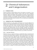
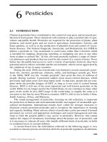
A vertical profile through soil, Figure 5.1, tells much about how the soil was formed.
It usually consists of a succession of more or less distinct layers, or strata. The layers
can form from aeolian or alluvial deposition of material, or from in situ weathering
processes.
5.2.1 SOIL HORIZONS
When the layers develop in situ by the weathering processes described above, they
form a sequence called horizons. The horizons are designated by the U.S. Depart-

ment of Agriculture by the capital letters: O, A, E, B, C, and R, in order of farthest
distance from the surface (see Figure 5.1).
O-horizon: Organic
.
The top horizon: starts at the soil surface
.
Formed from surface litter
.
Dominated by fresh or partly decomposed organic matter
O-horizon
A-horizon
E-horizon
B-horizon
C-horizon
R-layer
Surface litter: Fresh and partly
decomposed organic matter
Topsoil (rizosphere): Dark color,
finely divided, decomposed organic
matter, humus, roots, microbes,
insects, less soluble minerals
Leaching zone: Light color
Subsoil: Dark color, accumulated
minerals and humus leached
from upper horizons
Soil parent material: Fragmented
and weathered rock
Bedrock: Impenetrable layer,
except for fractures
FIGURE 5.1 Generalized soil profile showing the horizon sequence.

ß 2007 by Taylor & Francis Group, LLC.
A-horizon: Topsoil
.
The zone of greatest biological activity (rhizosphere)
.
Contains an accumulation of finely divided, decomposed, organic matter,
which imparts a dark color
.
Clays, carbonates, and most metal cations are leached out of the A-horizon
by downward percolating water; less soluble minerals (such as quart z) of
sand or silt size become concentrated in the A-horizon
E-horizon: Leaching zone (sometimes called the A-2 horizon)
.
Light-colored region below the rhizosphere where clays and metal cations
are leached out and organic matter is sparse
B-horizon: Subsoil
.
Dark-colored zone where downward migrating materials from the A-horizon
accumulate
C-horizon: Soil parent material
.
Fragmented and weathered rock, either from bedrock or base material that
has deposited from water or wind
R-layer: Bedrock
.
Below all the horizons; consists of consolidated bedrock
.
Impenetrable, except for fractures
5.2.2 SUCCESSIVE STEPS IN THE TYPICAL DEVELOPMENT OF A SOIL
AND

ITS PROFILE (PEDOGENESIS)
1. Physical disintegration (weather ing) of exposed rock formations forms the
soil parent material, the C-horizon.
2. The gradual accumulation of organic residues near the surface begins to
form the A-horizon, which might acquire a granular structure, stabilized to
some degree by organic matter cementation. This process is retarded in
desert regions where organic growth and decay are slow.
3. Continued chemical weathering (oxidation, hydrolysis, etc.), dissolution,
and precipitation b egin to form clays.
4. Clays, soluble salts, chelated metals, etc. migrate downward through the
A-horizon, carried by permeating water, to accumulate in the B-horizon.
5. The C-horizon, now below the O-, A-, and B-horizons, continues to
undergo physical and chemical weathering, slowly transforming into
B- and A-horizons, deepening the entire horizon structure.
6. A quasi-stable condition is approached in which the opposing processes of
soil formation and soil erosion are more or less balanced.
5.3 ORGANIC MATTER IN SOIL
Soil organic matter influences the weathering of minerals, provides food for soil
organisms, and provides sites to which ions are attracted for ion exchange. Only two
ß 2007 by Taylor & Francis Group, LLC.
types of organisms can synthesize organic matter from nonorganic materials. These
are certain bacteria called autotrophs and chlorophyll-containing plants. Organic
matter is developed in soil from the metabolism, wastes, and decay products of
plants and soil organisms. For example, soil fungi metabolism produces excellent
complexing agents such as oxalate ion and citric and other chelating organic acids.
These promote the dissolution of minerals and increase nutrient availability. Some
soil bacteria release the strong organic chelating agent 2-ketogluconic acid. This
reacts with insoluble metal phosphates to solubilize the metal ions and release
soluble phosphate, a plant nutrient.
As another example, oxalate ion is a metabolite of certain soil organisms. In

calcium soils, oxalate forms calcium oxalate, Ca(C
2
O
4
), which then reacts with
precipitated metals (particularly Fe or Al) to complex and mobilize them. The
reaction with precipitated aluminum is
3H
þ
þ Al(OH)
3
(s) þ 2Ca(C
2
O
4
) ! Al(C
2
O
4
)
À
2
(aq) þ 2Ca
2þ
(aq) þ 3H
2
O(5:1)
Because hydrogen ions are consumed, this reaction raises the pH of acidic soil.
It also weathers minerals by dissolving some metals and provides Ca
2þ

as a plant
and biota nutrient. Similar processes with silicate minerals release K
þ
and other
nutrient cations.
The amount of organic matter in soil has a stro ng influence on soil properties and
on the behavior of soil contaminants. For example, plants compete with soil for
water. In sandy soils, pore space is large and particle surface area is small. Water is
not strongly adsorbed to sands and is easily available to plants. However, in sandy
soils the water drains off quickly. On the other hand, water binds strongly to organic
matter in soil. Soils with high organic content hold more water; but the water is less
available to plants.
5.3.1 HUMIC SUBSTANCES
The most important organic substance in soil is humus , a collection of variously
sized polymeric molecules consisting of soluble fractions (humic and fulvic acids)
and an insoluble fraction (humin). Humus is the near-final residue of plant biodeg-
radation and consists largely of protein and lignin. Humus is what remains after the
more easily degradable components of plant biomass have degraded, leaving only
the parts most resistant to further degradation. Humic materials are not well-defined
chemically and have variable composition. Percent by weight for the most abundant
elements are C: 45%–55%, O: 30%–45%, H: 3%–6%, N: 1%–5%, and S: 0%–1%.
RULE OF THUMB
Organic matter is typically less than 5% in most soils, but is critical for plant
productivity. Peat soils can be 95% organic matter. Mineral soils can be less
than 1% organic matter.
ß 2007 by Taylor & Francis Group, LLC.
The exact chemical structure depends on the source plant materials and the history of
biodegradation.
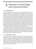
Humic and fulvic acids are soluble organic acid macromolecules containing
many –COOH and –OH functional groups that ionize in water, releasing H

þ
ions and providing negative charge centers on the macromolecule to which
cations are strongly attracted (see Figure 5.2). Humic materials are the most
important class of natural soil complexing agents and are found where vegetation
has decayed.
5.3.2 SOME PROPERTIES OF HUMIC MATERIALS
5.3.2.1 Binding to Dissolved Species
Humic materials are effective at removing metals from water by sorption to negative
charge sites, mainly at the structural oxygen atoms. Polyvalent metal cations are
sorbed especially strongly. The cation-exchange capacity of humic materials can be
as high as 500 meq=100 mL. Humic materials may sorb metals like uranium in
concentrations 10,000 times greater than adjacent water. Humic materials also bind
organic pollutants, especially low-solubility compounds like DDT and atrazine.
Much of the utility of wetlands for water treatment arises from their high concen-
trat ions of humi c mate rials. Figure 5.3 shows severa l ways by which metal cations
bind to humic and fulvic acids.
5.3.2.2 Light Absorption
Humic materials absorb sunlight in the blue region (transmitting yellow) and
can transfer the solar energy to sorbed molecules, initiating reactions. This
energy trans fer process can be effective in degrading pesticides and other organic
compounds.
H
3
C
CO
O
H
C
C
C

O
O
H
H
O
C
C
C
CH
3
H
C
C
O
O
H
C
O
O
H
H
O
H
CH
2
O
H
C
O
H

O
H
C
O
H
O
CC
O
O
H
O
O
H
H
FIGURE 5.2 Characteristic structural portion of an unionized humic or fulvic acid.
ß 2007 by Taylor & Francis Group, LLC.
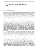
5.4 SOIL ZONES
In discussions of groundwater movement, the soil subsurface is commonly divided
into three zones, based on their air and water content (see Figure 5.4). From the
ground surface down to an aquifer water table, soils contain mostly air in the pore
spaces, with some adsorbed and capillary-held water. This region is called the water-
unsaturated zone or vadose* zone. From the top of the water table to bedrock, soils
contain mostly water in the pore spaces. This region is called the saturated zone.
C
O
O
O
M
C
O

C
O
O
O
M
C
O
O
M
+
(a) Chelation between
carboxyl and hydroxyl
groups
(b) Chelation between
two carboxyl groups
(c) Complexation with
carboxyl group
FIGURE 5.3 Some types of binding metal ions (M
2þ
) to humic or fulvic acids.
Bedrock
Water-unsaturated zone (vadose zone)
Water-saturated zone
Water table
Capillary zone
Ground surface
FIGURE 5.4 Soil zones in the subsurface region.
* From the Latin vadosus, meaning shallow.
ß 2007 by Taylor & Francis Group, LLC.
Between the vadose and saturated zones, there is a transition region called the

capillary zone, where water is drawn upward from the water table by capillary forces.
The thickness of the capillary zone depends on the soil text ure—the smaller the pore
size, the greater the capillary rise. In fine gravel (2–5 mm grain size), the capillary
zone will be of the order of 2.5 cm thick. In fine silt (0.02–0.05 mm grain size), the
capillary zone can be 200 cm or greater.
The saturated zone lies above the solid bedrock, which is impermeable except for
fractures and cracks. The region of the subsurface overlying the bedrock is generally
unconsolidated porous, granular mineral material.
5.4.1 AIR IN SOIL
Air in soil has a different composit ion from atmospheric air because of biodegrad-
ation of organic matter by soil organisms. Biodegradation occurs in many small
steps, but the net overall reaction is shown in Equation 5.2, where organic matter in
soil is represented by the approximate generic unit formula {CH
2
O}. An actual
molecule of soil organic matter would have a formula that is approximately some
whole number multip le of the {CH
2
O} unit.
{CH
2
O} þ O
2
! CO
2
þ H
2
O(5:2)
Equation 5.2 shows that, for each {CH
2

O} unit contained within a large r organic
molecule, one CO
2
molecule and one H
2
O molecule are produced by biodegradation.
Oxygen from soil p ore space air is consumed and CO
2
released by microbial
metabolism. Much of the soil air is semitrapped in pores and cannot readily equili-
brate with the atmosphere. As a result, the O
2
content in soil pore space air is
decreased from its atmospheric value of 21% to about 15% and CO
2
content
is increased from its atmospheric value of about 0.03% to about 3%. This, in turn,
increases the dissolved CO
2
concentration in groundwater, making it more acidic.
Acidic groundwater contributes to the weathering of soils, especially calcium
carbonate (CaCO
3
) minerals.
When soil becomes water-saturated, as in the saturated zone, many changes
occur:
1. Oxygen becomes used up by respiration of microorganisms.
2. Anaerobic processes lower the oxidation potential of water so that reduci ng
conditions (electron gain) prevail, whereas oxidizing conditions (electron
loss) dominate in the unsaturated zone.

3. Certain metals, particularly iron and manganese, become mobilized by chem-
ical reduction reactions that change them from insoluble to soluble forms:
Fe(OH)
3
(s) þ 3H
þ
þ e
À
! Fe
þ2
(aq) þ 3H
2
O(5:3)
Fe
2
O
3
(s) þ 6H
þ
þ 2e
À
! 2Fe
þ2
(aq) þ 3H
2
O(5:4)
MnO
2
(s) þ 5H
þ

þ 2e
À
! Mn
þ2
(aq) þ 2H
2
O(5:5)
ß 2007 by Taylor & Francis Group, LLC.
Groundw ater, moving under gravi ty, can transport dissolved Fe
þ 2
and Mn
þ 2
into
zones wher e oxidi zing condition s prevai l, e.g., by surfa cing to a spring, stream, or
lake. There, Equati ons 5.3 throu gh 5.5 are revers ed a nd the met als redepos it as solid
precipitates, mainly Fe(OH)
3
and MnO
2
. Precipitation of Fe(OH)
3
often causes ‘‘red
water’’ and red or yellow deposits on rocks and soil. MnO
2
deposits are black. These
deposits can clog underdrains in fields and water treatment filters.
5.5 CONTAMINANTS BECOME DISTRIBUTED IN WATER,
SOIL, AND AIR
In the environment, contaminants always contact water, air, and soil. No matter
where it originated, a contaminant moves across the interfaces between water, soil,

and air phases to become distributed, to different degrees, into every phase it
contacts. Partitioning of a pollutant from one phase into other phases serves to
deplete the concentration in the original phase and increase it in the other phases.
The movement of contaminants throu gh soil is a process of continuous redistribution
among the different phases it encounters. It is a process controlled by gravity,
capillarity, sorption to surfaces, miscibility with water, and volatility.
5.5.1 VOLATILIZATION
The main partitioning process from liquids and solids to air is volatilization, which
moves a contaminant across the liquid–air or solid–air interface into the atmosphere
or into air in soil pore spaces. Volatilization is an important partitioning mechanism
for compounds with high vapor pressures. For liquid mixtures such as gasoline, the
most volatile components are lost first, causing the composition and properties of
the remaining liquid mixture to change over time. For example, the most volatile
components of gasoline are generally the smallest molecules in the mixture. The
remaining larger molecules have stronger London attractive forces. Hence, as gas-
oline weathers and loses the smaller molecules by volatilization, its vapor pressure
decreases and its viscosity and density increase.
5.5.2 SORPTION
The main partitioning process from liquids and air to solids is sorption, which moves
a contaminant across the liquid–solid or air–solid interface to organic or mineral
solid surfaces. Sorption from the water phase is most important for compounds of
low solubility. Once a contaminant is sorbed to a surface, it undergoes chemical and
biological transformations at different rates and by different pathways than if it
were dissolved.
EXAMPLE 1
ESTIMATING SOME RELATIVE PHYSICAL PROPERTIES
Suppose you need to compare the relative vapor pressures, water solubilities, and
Henry’s law constants of the compounds tabulated below, but are only able to find
ß 2007 by Taylor & Francis Group, LLC.
melting point data. Estimate their relative values of these parameters based on their

melting points and structures.
.
Vapor pressure (P
v
) is a measure of the tendency for molecules to partition
from a pure substance into the atmosphere.
.
Solubility (S
w
) is a measure of the tendency of molecules to partition from a
pure substance into water.
.
Henry’s law constant (K
H
) is a measure of a compound’s tendency to partition
between water and air. It may be considered to be the vapor pressure of a
substance dissolved in water.
Compound Structure
Phenol
Melting temp. ¼ 41.08C
OH
1,2,3,5-Tetrachlorobenzene
Melting temp. ¼ 54.58C
Cl
Cl
Cl
Cl
1,2,4,5-Tetrachlorobenzene
Melting temp. ¼ 1408C
Cl

Cl
Cl
Cl
Answer:
Vapor pressure varies inversely with intermolecular attraction. Substances with high
vapor pressure have weak intermolecular attractive forces. Therefore, vapor pressure
will tend to vary inversely with melting point, because a high melting point indicates
strong intermolecular attractive forces.*
Solubility varies with polarity and the ability to form hydrogen bonds to water
molecules. The more polar the molecule and the more hydrogen bonding to water, the
more soluble it will be, because of stronger attraction to water molecules. It also varies with
* The correspondence between melting point and vapor pressure is only approximate, because the melting
point may also depend on the crystal lattice energy, a function of the molecular geometry of the solid.
However, it can serve as a first approximation where more accurate data are not available.
ß 2007 by Taylor & Francis Group, LLC.
molecular weight. Higher molecular weight tends to decrease a compound’s solubility
because London attractive forces are stronger, attracting the compound molecules to one
another more strongly.
Henry’s law constant depends on two different properties of a substance. It varies
inversely with solubility and directly with vapor pressure. In general, solubility will
dominate in determining K
H
.
Vapor pressure: (Lowest to highest vapor pressure will be, to a first approximation, in
the order of highest to lowest melting point.)
1,2,4,5-tetrachlorobenzene < 1,2,3,5-tetrachlorobenzene < phenol
Solubility: (Lowest to highest solubility will be in the order of lowest to highest
polarity, highest to lowest molecular weight, and fewest to most hydrogen bonds
to water.)
Least soluble is 1,2,4,5-tetrachlorobenzene (nonpolar because of symmetry; high

molecular weight, no hydrogen bonds).
More soluble is 1,2,3,5-tetrachlorobenzene (less symmetrical, therefore more
polar; same molecular weight as 1,2,4,5-tetrachlorobenzene, no hydrogen
bonds).
Most soluble is phenol (most polar; the only compound that can form hydrogen
bonds to water; lightest molecular weight of all).
Henry’s law constant: Lowest to highest K
H
should vary according to highest to lowest
solubility and lowest to highest vapor pressure. Phenol, with the highest polarity,
greatest solubility and lowest melting point, will have the lowest K
H
. Because the
solubilities of 1,2,3,5-tetrachlorobenzene and 1,2,4,5-tetrachlorobenzene are so similar,
their K
HS
are expected to be similar also. However, their vapor pressures differ by a
factor of more than 10. The much higher vapor pressure of 1,2,3,5-tetrachlorobenzene
might give it a slightly higher K
H
than 1,2,4,5-tetrachlorobenzene.
Phenol < 1,2,4,5-tetrachlorobenzene < 1,2,3 ,5-tetrachlorobenzene
The measured values in Table 5.1 confirm these relative vapor pressure, solubility, and
K
H
estimates.
TABLE 5.1
Measured Values for Melting Point, Vapor Pressure, Solubility,
and Henry’s Law Constant
MW T

m
P
v
S
w
K
H
Compound (g) (8C) (atm) (mg=L) (atm m
3
=mol)
Phenol 94.1 41.0 2.6 3 10
À4
8,2000 4.0 3 10
À7
1,2,3,5-Tetrachlorobenzene 215.9 54.5 1.4 3 10
À5
3.5 5.8 3 10
À3
1,2,4,5-Tetrachlorobenzene 215.9 140.0 5.3 3 10
À6
2.2 2.6 3 10
À3
Note: T
m
¼ melting point; P
v
¼ vapor pressure; S
w
¼ solubility in water; K
H

¼ Henry’s law constant.
ß 2007 by Taylor & Francis Group, LLC.
EXAMPLE 2
Rank the four compounds below in order of increasing Henry ’ s law constant (tendency
to partition from water into air).
Cl
C
H
H
H
O
C
H
H
H
H
N
C
H
H
H
H
H
O
C
H
H
H
C
H

H
H
I II III IV
1-chloro-3- 3-methylphenol 3-methylaniline 3-methylanisole
methylbenzene (m-cresol)
Answer :
All the compounds are similar in molecular weight and their structures differ only in the
top functional group. The molecule having the group with the weakest attractive force
to water will most readily partition from water into air. Therefore, we want to rank them
by their relative attractions to water, i.e., solubilities.
I. Has no oxygen, nitrogen, or fluorine for H-bonding to water and is the least
polar. It will volatilize the most readily.
IV. Has an oxygen, but no hydrogen is attached to it for H-bonding to water. It
will be next in volatility from water to air.
II. and III. Both can H-bond. II can form one H-bond while III can form two
H-bonds, so, II is third in volatility and III is the least volatile in water.
Order of Henry’s law constants: I > IV > II > III
Their measured Henry ’ s law constants (dimensionless) are
I, K
H
¼ 1:38; IV, K
H
¼ 1:17; II, K
H
¼ 0:0034; III, K
H
¼ 0:0015
A larger Henry’s law constant means greater tendency to volatilize from water
(see Section 5.6.1).
5.6 PARTITION COEFFICIENTS

The tendency for a pollutant to move from one phase to another is often quantified by
the use of a partition coefficient, also called a distribution coefficient. Partition coeffi-
cients are chemical specific. They can be measured directly or, in some cases, estimated
from other properties of the chemical. The simplest form of a partition coefficient is the
ratio of the pollutant concentration in phase 1 to its concentration in phase 2:
K
1,2
¼
concentration in phase 1
concentration in phase 2
¼
C
1
C
2
(5:6)
This expression assumes that a linear relation exists between the concentrations of
a substance in different phases, and is often satisfactory for low to moderate
ß 2007 by Taylor & Francis Group, LLC.
concentrations. The phase of the denominator, C
2
, is referred to as the reference
phase. Water is commonly used as the reference phase to maintain some consistency
in published values. Using water as the reference phase, a linear relation gives
Equations 5.7 through 5.9 for partitioning between water and air, water and free
product (original physical form of the pollutant, such as a layer of oil floating on a
river or above the groundwater table; sometimes called the bulk pollutant), and water
and soil. In these equations, the pollutant may be a pure substance, like benzene, or
one component from a mixture, like benzene from free product liquid gasoline.
C

a
¼ K
H
C
w
(5:7)
K
H
is the air–water partition coefficient, also known as Henry’s law const ant. C
a
and
C
w
are the pollutant concentrations in air and water, respectively.
C
p
¼ K
p
C
w
(5:8)
K
p
is the free product–water partition coefficient. C
p
and C
w
are the pollutant
concentrations in the free product and water, respectively.
C

s
¼ K
d
C
w
(5:9)
K
d
is the soil–water partition coefficient. C
s
and C
w
are the pollutant concentrations
sorbed on soil and dissolved in water, respective ly.
Each value of K depends on properties of the particular pollutant and the
temperature. K
d
also depends on the type of soil.
5.6.1 AIR–WATER PARTITION COEFFICIENT (HENRY’S LAW)
Henry’s law, C
a
¼ K
H
C
w
, describes how a substance distributes itself at equilibrium
between water and air. The units of Henry’s law constant, K
H
¼ C
a

=C
w
, depends on
what units are used to express concentrati ons in air and water.* For the case of
oxygen gas, O
2
,at208C
.
When air and water concentrations both have the same units,
K
H
(O
2
,20

C) ¼ 26 (unitless) (5:10)
.
For water concentration in mol=L or mol=m
3
, and air in atmosphere s,
K
H
(O
2
, 20

C) ¼ 635 LÁ atm=mol ¼ 0:635 m
3
Áatm=mol (5:11)
.

For water concentration in mg=L and air in atmospheres,
K
H
(O
2
, 20

C) ¼ 0:0198 LÁatm=mg (5:12)
* Henry’s law constants are tabulated in many references, such as Handbook of Chemistry and Physics,
CRC Press; Howard (1991); Lyman et al. (1990); Mackay and Shiu (1981); Sander (1999). There are
also computer programs that calculate Henry’s law constant from other chemical properties.
ß 2007 by Taylor & Francis Group, LLC.
EXAMPLE 3
If soil pore water is measured to contain 3.2 mg=L of oxygen at 208C, what is the
concentration, in mg=L and in atmospheres, of oxygen in the air of the soil pore space?
Answer :
For O
2
at 20

C, K
H
¼ 26 ¼
C
a
3: 2 mg =L
; C
a
¼ ( 26)(3: 2 mg=L) ¼ 83: 2mg=L
Using different units,

K
H
¼ 0: 0198 L Á atm =mg ¼
C
a
3:2 mg= L
C
a
¼ ( 0: 0198 L Á atm =mg)(3: 2mg=L) ¼ 0:063 atm
Since the normal atmospheric partial pressure of oxygen at sea level is about 0.2 atm,
this result, showing that the soil oxygen concentration is lower than atmospheric,
indicates the presence in the soil of microbial activity that has consumed oxygen.
EXAMPLE 4
BO D AND H ENRY ’ S LAW
A certain sewage treatment plant located on a river typically removes 100,000 lb
(4.54 3 10
7
g) of biodegradable organic waste each day. If there were a plant upset
and it became necessary to release one day’ s waste into the receiving river, how many
liters of river water could potentially be contaminated to the extent of totally depleting
the water of all oxygen?
Answer :
An approximate chemical equation we have used before (Section 5.4.1) as being
suitable for biodegradation of organic matter is
{CH
2
O} þ O
2
! CO
2

þ H
2
O(5: 2)
Assume the river water is initially saturated with oxygen from the air at 208 C and that,
after the spill, no additional oxygen dissolves from the atmosphere, a worst case scenario.
Necessary Data:
Atm. pressure at the treatment plant ¼ 0.82 atm
Vapor pressure of water at 208C ¼ 0.023 atm
Percent O
2
in dry air ¼ 21%
From Equation 5.11, K
H
(O
2
) ¼ 635 LÁatm=mol
Calculation:
Organic matter is biodegraded, consuming oxygen by Equation 5.2. This chemical
equation shows that one mole of O
2
is consumed for each mole of CH
2
O biodegraded.
The molecular weight of CH
2
Ois30g=mol. Therefore,
Moles of CH
2
O in sewage ¼
4:54 Â 10

7
g
30 g=mol
¼ 1:5 Â 10
6
mol ¼ moles of O
2
consumed
ß 2007 by Taylor & Francis Group, LLC.
Atmospheric pressure ¼ P
total
¼ 0:82 atm ¼ P
O
2
þ P
N
2
þ P
H
2
O
P
dry air
¼ atmospheric pressure partial pressure of water vapor ¼ P
total
P
H
2
O
Therefore, P

O
2
¼ (0:21)(P
total
P
H
2
O
) ¼ (0:21)(0:82 atm 0 :023 atm) ¼ 0:17 atm:
Use Henry’s law to find the concentration of dissolved O
2
in the river.
K
H
(O
2
) ¼ 635 LÁatm=mol ¼
C
a
C
w
¼
0:17 atm
C
w
C
w
¼ [O
2
(aq)] ¼

0:17 atm
635 atmÁL=mol
¼ 2:710
À4
mol=L
or [O
2
(aq)] ¼ (2:7 Â 10
À4
mol=L) Â (32 g=mol) ¼ 8:6mg=L
In saturated water at 208C and 0.82 atm total pressure, [O
2
, aq] ¼ 2.7310
À4
mol=L
Liters of river water depleted of O
2
¼
1:5 Â 10
6
mol O
2
consumed
2:7 Â 10
À4
mol O
2
=L in river
¼ 5:6 Â 10
9

L
This is a worst-case scenario. Less oxygen than calculated would be lost from the river
because of continuous replenishing of oxygen to the river by partitioning from
the atmosphere. The rate at which this occurs would depend on several factors such
as the surface to volume ratio of the river, water turbulence and cascades, wind velocity,
and temperature.
Note that both vapor pressure (proportional to C
a
) and solubility (proportional to C
w
)
of a pure solid or liquid generally increase with temperature, but vapor pressure always
increases faster. Therefore, the value of K
H
increases with temperature, indicating that,
for a gas partitioning between air and water, the atmospheric portion increases and the
dissolved portion decreases when the temperature rises. This is consistent with
the observation that the water solubility of gases decreases with increasing temperature.
RULE OF THUMB
Estimating K
H
:
If a tabulated value for K
H
cannot be found, it may be estimated roughly by
dividing the vapor pressure of a compound by its aqueous solubility. For some
compounds, tabulated values of vapor pressure and solubility may be easier to
find than K
H
values.

K
H
¼
C
a
(partial pressure in atmospheres)
C
w
(mol=L)
%
vapor pressure (atm)
aqueous solubility (mol=L)
(5:13)
In this case, the units of K
H
are atm Á L mol
À1
ß 2007 by Taylor & Francis Group, LLC.
EXAMPLE 5
Estimate Henry ’ s law constants for chlorobenzene and bromomethane using vapor
pressure and aqueous solubility.
Chlorobenzene: P
v
(258 C) ¼ 1.6 3 10
À 2
atm;
C
w
(258 C) ¼ 4.5 3 10
À3

mol=L
Cl
K
H
(258 C) % P
v
=C
w
¼ 1.6 3 10
À2
atm=4.5 3 10
À3
mol=L
¼ 3.6 L Á atm=mol
This happens to exactly match the experimental value. To put K
H
into
dimensionless form, divide by RT (R ¼ universal gas constant,
T ¼ temperature in degrees Kelvin), equivalent to multiplying by
0.041 mol=LÁatm:
K
0
H
¼
3:6 L Á atm=mol
( 0:0821 L Á atm=mol K)( 298 K)
¼ 0:15
Bromomethane: P
v
(liq, 258 C) ¼ 1.8 atm;

C
w
(1 atm, 258 C) ¼ 0.16 mol=L.
C
Br
H
H
H
At 25 8C, bromomethane has a vapor pressure > 1 atm, so it is a gas.
Since the solubility is given at 1 atm partial pressure, all gases should
be used at a vapor pressure of 1 atm.
K
H
(258 C) % P
v
=C
w
¼ 1 atm=0.16 mol=L ¼ 6.3 LÁatm=mol
K
0
H
¼
6:3 L Á atm=mol
( 0:0821 L Á atm=mol K) (298 K)
¼ 0:26
EXAMPLE 6
Estimate relative Henry ’ s law constants for the compounds in Example 1 using vapor
pressure and solubility data from Table 5.1. Compare your answer with the measured
K
H

values in Table 5.1.
Answer :
From Equation 5.13, Henry ’s law constant varies directly with vapor pressure and
inversely with aqueous solubility.
K
H
%
vapor pressure (atm)
aqueous solubility (mol=L)
Use vapor pressure and solubility data from Table 5.1 to estimate approximate Henry’ s
law values.
K
H
(phenol) %
2:6 Â 10
À4
atm
8:2 Â 10
4
mg=L
Â
94:1 g=mol
10
À3
g=mg
¼ 3:0 Â 10
À4
LÁatm=mol
K
H

(1,2,3,5-tetrachlorobenzene) %
1:4 Â 10
À5
atm
3:5 mg=L
Â
215:9 g=mol
10
À3
g=mg
¼ 0:86 LÁatm=mol
ß 2007 by Taylor & Francis Group, LLC.
K
H
(1,2,4,5-tetrachlorobenzene) %
5:3 Â 10
À6
atm
2:2 mg =L
Â
215:9 g=mol
10
À3
g=mg
¼ 0:52 LÁatm=mol
K
H
(1,2,3,5-tetrachlorobenzene) > K
H
(1,2,4,5-tetrachlorobenzene) >> K

H
(phenol)
Table values:*
K
H
(phenol) ¼ 4: 0 Â 10
À4
LÁatm=mol
K
H
(1,2,3,5-tetrachlorobenzene) ¼ 5:8 LÁatm=mol
K
H
(1,2,4,5-tetrachlorobenzene) ¼ 2:6 LÁatm=mol
The calculated value for phenol is very close to the measured value. The calculated values
for the chlorobenzenes are in the correct order but are about one-fifth too small. It cannot
be determined why the calculated values for 1,2,3,5-tetrachlorobenzene and 1,2,3,5-
tetrachlorobenzene differ from the measured values without examining the original experi-
mental data. It is likely due to experimental error based on the difficulty of accurately
measuring such low pressures. This could also explain why the Henry’s law constant of the
polar 1,2,3,5-tetrachlorobenzene appears to be higher than that of the nonpolar 1,2,4,5-
tetrachlorobenzene. The absolute difference in the constants is small and could be
accounted for by the limits of error in the vapor pressure measurements, where an
uncertainty factor of 3 or 4 is not unusual in tabulated values of small vapor pressures.
It might seem counterintuitive that phenol, the compound with the highest vapor
pressure in the pure state, has the lowest Henry’s law constant. This example shows the
importance of the environment immediately surrounding the molecule. Phenol is much
more strongly attracted to water molecules than to other phenol molecules. Consequently, it
enters the vapor state more readily from pure liquid phenol than from a water solution.
5.6.2 SOIL–WATER PARTITION COEFFICIENT

Partitioning from water into soil surfaces can be limited by the available soil surface
area. The rate of transfer will slow as the soil surface becomes saturated. For this
reason, the partitioning of a compound between water and soil may deviate from
linearity. This is particularly true for the partitioning of organic compounds. To
account for nonlinearity, the corresponding partition coefficient is often written in a
modified form called the Freundlich isotherm. The modification consists in introdu-
cing an empirically determined exponent to the C
w
term.
C
s
¼ K
d
C
n
w
(5:14)
where
C
s
is the concentration of sorbed organic compound in solid phase (mg=kg)
C
w
is the concentration of dissolved organic compound in water phase (mg=L)
K
d
¼ C
s
=C
w

n
is the partition coefficient for sorption
n ¼ empirically determined exponential factor
* Reference: Canadian Water Quality Guidelines, Task Force on Water Quality Guidelines of the
Canadian Council of Resource and Environment Ministers, March 1987.
ß 2007 by Taylor & Francis Group, LLC.
When C
w
( C
s
(the common case for organic compo unds of low water
solub ility) , then n is close to unit y for most organi cs. However , n typi cally is
temperature dependent.
Equation 5.14 can be writt en as an equation for a straight line by takin g the
logarithm of both sides, as in
log C
s
¼ log K
d
þ n log C
w
(5:15)
It is important not to extrapolate the Freundlich isotherm too far beyond the range of
experimental data.
EXAMPLE 7
USE OF THE FREUNDLICH ISOTHERM
A power company planned to discharge their power plant cooling water into a small
lake. Before purchasing the lake, they tested the water and found the pesticide 2,4-D
(2,4-dichlorophenoxyacetic acid) at 0.8 ppt (0.8 parts per trillion, or 0.8 3 10
À9

g=L),
just a little below the permitted limit of 1 ppt. The company calculated that their
operation would raise the water temperature in the mixing zone near their discharge
from 58C to about 258C. Should they anticipate a problem?
Answer:
2,4-D has low solubility and is denser than water. It will sink in the lake and become sorbed
on the bottom sediments. The potential problem is whether the expected increase in
temperature will cause the 2,4-D limit to be exceeded because of additional 2,4-D partition-
ing into the water from the bottom sediments. It is a case for the Freundlich isotherm,
because the empirical constant n is a function of temperature and will cause a change in K
d
when the temperature changes. A Web search found a study (Means and Wijayratne, 1982)
that measured Freundlich isotherm values for 2,4-D at 58Cand258C (Table 5.2).
C
s
¼ K
d
C
n
w
(5:14)
At 5

C: C
s
¼ (6:53)(0:8 Â 10
À9
g=L)
0:76
¼ (6:53)(1:22 Â 10

À7
) ¼ 797 Â 10
À9
g=kg
The calculation indicates that there are 797 ppt of 2,4-D sorbed on the sediments at 58C.
Note that the concentration of 2,4-D sorbed to sediments is about 1000 times larger
than the dissolved concentration. Even if a temperature rise to 258C causes a large
percentage increase in the dissolved portion, the percentage loss from the sediment
fraction will be 1000 times smaller. Assume that the sediment concentration at 258Cis
essentially the same as at 58C. This allows an approximate calculation of C
w
at 258C.
TABLE 5.2
Values for Freundlich Isotherm Parameters of 2,4-D
Temperature (8C) nK
d
log K
d
5 0.76 6.53 0.815
25 0.83 5.20 0.716
ß 2007 by Taylor & Francis Group, LLC.
At 25

C: 797 Â 10
À9
g= kg ¼ ( 5: 20)( C
w
)
0:83
C

w
( 25

C) ¼
797 Â 10
À9
5:20

1
0 :83
¼ 6: 2 Â 10
À 9
g=L ¼ 6: 2 ppt
The expected temperature rise will cause 2,4-D to desorb from the bottom sediments
and raise the water concentration well over the permitted limit of 1 ppt.
5.6.3 DETERMINING K
D
EXPERIMENTALLY
The Freundl ich Equa tion 5.14 can be used to deter mine K
d
experimentally, as
follows:
1. Prepare samples having several different concentrations of dissolved
contaminant in equilibrium with soil from the site of interest.
2. Measure the contaminant concentrations in water, C
w
, in each sample.
3. Measure the corresponding contaminant concentrations sorbed to soil, C
s
.

4. Plot log C
s
versus log C
w
to get a straight line with slope ¼ n and
intercept ¼ log K
d
.
EXAMPLE 8
Prepared water samples containing different concentrations of benzene were equili-
brated with clean soil from a site under study. Equilibrium concentrations of dissolved
and sorbed benzene are shown in Table 5.3. Find K
d
for benzene in this soil.
TABLE 5.3
Benzene Partitioning Data for Soil and Water
in Equilibrium
Dissolved Benzene C
w
(mg=L) Sorbed Benzene C
s
(mg=kg)
6.59 2.2
10.00 3.1
33.28 8.1
34.57 9.6
68.31 15.00
88.89 26.00
183.74 44.00
340.54 89.00

452.30 119.00
674.79 130.00
819.56 188.00
955.95 247.00
ß 2007 by Taylor & Francis Group, LLC.
Answer:
1. Determine the base-10 logarithms of all the concentration values.
Logarithms of C
w
and C
s
log C
w
log C
s
0.819 0.342
1.000 0.491
1.522 0.908
1.539 0.982
1.834 1.176
1.949 1.415
2.264 1.643
2.532 1.949
2.655 2.076
2.829 2.114
2.914 2.274
2.980 2.393
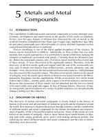
2. Plot log C
w
versus log C

s
and fit a straight line through the points. The
formula of the line is log C
s
¼ log K
d
þ n log C
w
. Therefore, the slope of the
line is equal to n and the y-axis intercept is equal to log K
d
. The resulting plot
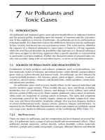
is shown in Figure 5.5.
The equation of the least-squares fitted line is log C
s
¼ 0.941 log C
w
À 0.468.
1.0 1.5
log C
w
log C
s
2.0 2.5 3.0 3.50.50.0
0.0
0.5
1.0
1.5
2.0
2.5

3.0
y
= 0.9414x − 0.468
R
2
= 0.9949
FIGURE 5.5 Freundlich isotherm for benzene partitioning between water and soil.
ß 2007 by Taylor & Francis Group, LLC.
Therefore,
n ¼ 0:941
log K
d
¼À0:468
K
d
¼ 0:340 L=kg
5.6.4 ROLE OF SOIL ORGANIC MATTER
Values for K
d
are extremely site- and chemical specific because the extent of sorption
depends on several physical and chemical properties of both the soil and the sorbed
chemical. For dissolved neutral organic molecules, such as fuel hydrocarbons,
sorption to soils is controlled mostly by sorption to the organic portion of the soil.
Therefore, the value of the soil–water partition coefficient, K
d
, depends on the
amount of organic matter in the soil. Expressing the soil–water partition coefficient
in terms of soil organic carbon (K
oc
), rather than total soil mass (K

d
), can eliminate a
large part, but not all, of the site-specific variability in K
d
.
The amount of organic matter in soil is usually expressed as either the weight
fraction of organic carbon, f
oc
, or the weight fraction of organic matter, f
om
. The
amount of organic matter in typical mineral soils is generally between about 1% and
10%, but is typically less than 5%. In wetlands and peat-soils, it can approach 100%.
Since soil organic matter is approximately 58% carbon, f
oc
typically ranges between
0.006 and 0.06. Some characteristic values of f
oc
for a range of different soil types
are given in Table 5.4.
There is a critical lower value for the fraction of organic carbon in the soil, f
*
oc
(dependent on the dissolved organic compound), below which sorption to inorganic
matter becomes dominant. Typical values for f
*
oc
are between about 10
À3
and 10

À4
(0.1%–0.01%).
TABLE 5.4
Typical Values of Fraction of Organic Carbon
in Different Soils
Type of Soil Typical f
oc
(wt. fraction)
Coarse soil 0.04
Silty loam 0.05
Silty clayey loam 0.03
Clayey silty loam 0.005
Clayey loam 0.004
Sand 0.0005
Glaciofluvial 0.0001
Note: These typical values were collected from many sources. They
should only be used as crude estimates when site-specific
measurements cannot be obtained. The range of measured values
for a single soil type can span a factor of 100.
ß 2007 by Taylor & Francis Group, LLC.
If we define K
oc
¼
C
oc
C
w
, where C
oc
is the concentration of contaminant sorbed to

organic carbon and C
w
is the concentration of contaminant dissolved in water, then
the soil–water partition coefficient becomes
K
d
¼ K
oc
f
oc
(5:16)
This relation is useful as long as f
oc
is greater than about 0.001.
EXAMPLE 9
Find K
oc
for benzene in the soil of Example 8. The soil contains 1.1% organic matter.
Answer:
The soil organic matter was measured to be 1.1%, or f
om
¼ 0.011. This may be
converted to fraction of organic carbon ( f
oc
) by the approximate rule of thumb
f
oc
¼ 0:58 f
om
Therefore, f

oc
¼ 0:58 Â 0:011 ¼ 0:0064: Since K
d
¼ K
oc
f
oc
, we have
K
oc
(benzene) ¼ 0:340=0:0064 ¼ 53 L=kg
5.6.5 OCTANOL–WATER PARTITION COEFFICIENT, K
OW
For laboratory experiments, the liquid compound octanol, an eight carbon organi c
alcohol, CH
3
(CH
2
)
7
OH, is a good surrogate for the organic carbon fraction of soils.
The partitioning behavior of organic compounds between octanol and water is
similar to that between the organic carbon fraction of soil and water. The basic
steps for measuring the octanol–water partition coefficient, K
ow
, are as follows:
1. Combine octanol and water in a bottle. Octanol forms a separate phase
floating on top of the water.
2. Add the organic contaminant (e.g., carbon tetrachloride, CCl
4

), shake
the mixture, and let the phases separate.
3. Measure the contaminant concentrations in the octanol phase and in the
water phase.
RULES OF THUMB
1. It is often found that typical soil organic matter is about 58% carbon.
Using this value to convert between the fraction of organic carbon
and the fraction of organic matter leads to the relation f
oc
% 0.58 f
om
.
2. Soil organic carbon content can vary by a factor of 100 for similar
soils. Although there have been tabulations of f
oc
values according to
soil type (e.g., Maidment, 1993), it is much better to use values
measured at the site for use in Equation 5.16.
ß 2007 by Taylor & Francis Group, LLC.
Then
K
ow
¼
C
octanol
C
water
( 5: 17 )
An empi rical equation that relates K
ow

and organic carbon to K
d
is
K
d
¼ f
oc
bK
a
ow
( 5: 18 a)
or
log K
d
¼ a log K
ow
þ log f
oc
þ log b (5 : 18b)
where the empirica lly determin ed constants a and b depend on the organic
compound.
Equati on 5.19, derived from Equ ations 5.16 and 5.18a , is a relation that allo ws a
calculation of K
oc
in terms of K
ow
.
K
oc
¼ bK

a
ow
(5:19)
The usefulness of these relations is evident in the rules of thumb for K
ow
. Knowing
the value of K
ow
for a compound allows one to qualitatively estimate many of its
environmental properties.
EXAMPLE 10
Consider the pesticide DDT in terms of the rules of thumb for K
ow
. For DDT,
K
ow
¼ 3.4 3 10
6
, which is well into the high value range for K
ow
. From the rules of
thumb, one can predict that DDT has low water solubility (its measured solubility is
25 mg=L), is slowly biodegraded, is persistent in the environment (low mobility and
slow biodegradation), is strongly adsorbed to soil, and is strongly bioaccumulated.
RULES OF THUMB FOR K
ow
(High K
ow
¼> 1000)
The higher K

ow
is for a compound
.
The higher is the sorption to soil
.
The higher is the bioaccumulation
.
The l ower is the biodegradation rate
.
The lower is the water solubility
.
The lower is the mobility
(Low K
ow
¼< 500)
The lower K
ow
is for a compound
.
The lower is the sorption to soil
.
The l ower is the bioacc umulation
.
The higher is the biodegradation
rate
.
The higher is the solubility
.
The higher is the mobility
ß 2007 by Taylor & Francis Group, LLC.

On the other hand, phenol has K
ow
¼ 30.2, a low value. Phenol has high water
solubility (its measured solubility is 8.3 3 10
4
mg=L), biodegrades rapidly, is not
persistent in the environment, is weakly sorbed to soil, is highly mobile, and is weakly
bioaccumulated.
5.6.6 ESTIMATING K
D
USING MEASURED SOLUBILITY OR K
ow
Literature values for K
d
measurements vary considerably because they are so site
specific. Considerable effort has been expended in finding more consistent
approaches to soil sorption. EPA has published a comprehensive evaluation of the
soil–water partition coefficient, K
d
(USEPA, 1999).
The following empirical observations have led to methods for estimating K
d
from more easily measured parameters:
.
Water solubility is inversely related to K
d
; the lower the solubility, the
greater is K
d
.

.
Since molecular polarity correlates with solubility, molecules whose
structure indicates low polarity (hence, low solubility) may be expected
to have a high K
d
.
.
For compounds of low solubility, such as fuel hydrocarbons, sorption is
controlled primarily by interactions with the organic portion of the solid
sorbent.
.
The surface area of the solid is important. The larger the surface area, the
larger will be K
d
.
.
A simple way to estimate the tendency for a compound to partition
between water and organic solids in the soil is to measure K
ow
, the
partition coefficient for the compound between water and octanol. The
larger is K
ow
, the larger is K
d
.
Because K
d
is site speci fic, it is generally preferable to calculate it from the more
easily obtained quantities K

ow
, K
oc
, f
oc
, and solubility. K
ow
and solubility (S) are easily
measured in a laboratory and K
oc
may be normalized to f
oc
, percent organic carbon in
soil, which is an easily measured site parameter. There are linear relationships
between log K
oc
, log K
ow
, and S (Lyman et al., 1990) that vary according to the
class of compounds tested (e.g., chlorinated compounds, aromatic hydrocarbons,
ionizable organic acids, pesticides, etc.). These relations can be used to calculate
K
oc
from K
ow
or S in the absence of measured K
oc
data. The EPA has reviewed the
soil–water partitioning literature and selected or calculated the most reliable values in
their judgment. In these calculations, EPA used the following relations.

For nonionizable, semivolatile organic compounds
log K
oc
¼ 0:983 log K
ow
þ 0:00028 (5:20)
For nonionizable, volat ile organic compounds
log K
oc
¼ 0:7919 log K
ow
þ 0:0784 (5:21)
ß 2007 by Taylor & Francis Group, LLC.
In addit ion, EPA sugges ts the use of the follow ing equ ation for estimat ing K
oc
from
solubili ty ( S) or biocon centra tion factors (BCF):
log K
oc
¼ 0: 681 log BCF þ 1: 963 ( 5: 22 )
Values for K
oc
, K
ow
, S, and BCF for many envir onmen tally importan t chemi cals
have been collected in look-up tables for use in EPA ’s soil screen ing guidan ce
procedu res (USEP A, 1996). Table 5.5 is ad apted from these EPA tabl es.
EXAMPLE 11
Benzene Spill :
A benzene leak soaked into a patch of soil. To determine how much benzene was in the

soil, several soil samples were taken in a grid pattern across the area of maximum
contamination. From analysis of these samples, the average benzene concentration in
the soil was 2422 mg=kg (ppm). The soil contained 2.6% organic matter. From
Table 5.5, log K
ow
(benzene) ¼ 2.13. If rainwater percolate down through the contam-
inated soil, what concentration of benzene might initially leach from the soil and be
found dissolved in the water? Assume the water and soil are in equilibrium with respect
to benzene.
Calculation :
The general approach to this type of problem is
1. Find a tabulated value of K
oc
for the chemical of concern, or calculate it from
tabulated values for K
ow
or S.
2. Obtain a measurement of f
oc
or f
om
in soil at the site or estimate it from the
soil type.
3. Calculate K
d
from the above quantities.
Benzene is a volatile, nonionizable organic compound (refer to Group 2 in Table 5.5).
Use K
d
¼

C
soil
C
w
¼ K
oc
f
oc
and Equation 5: 20:
log K
oc
¼ 0:7919 log K
ow
þ 0:0784
log K
oc
¼ 0:7919(2:13) þ 0:0784 ¼ 1:7651
K
oc
¼ 58:2
Since f
oc
% 0:58 f
om
¼ 0:58(0:026) ¼ 0:015, we have
K
d
¼
C
soil

C
w
¼ K
oc
f
oc
¼ 58:2(0:015) ¼ 0:88 L=kg
When 1 L of water is in equilibrium with 1 kg of soil, C
soil
þ C
w
¼ 2422 ppm.
ß 2007 by Taylor & Francis Group, LLC.