Ecosystem Responses to Mercury Contamination: Indicators of Change - Chapter 3 doc
Bạn đang xem bản rút gọn của tài liệu. Xem và tải ngay bản đầy đủ của tài liệu tại đây (837.42 KB, 40 trang )
47
3
Monitoring and
Evaluating Trends
in Sediment and
Water Indicators
David Krabbenhoft, Daniel Engstrom,
Cynthia Gilmour, Reed Harris, James Hurley,
and Robert Mason
ABSTRACT
As recently as a decade ago, a paucity of geographically dispersed and reliable data
on mercury (Hg) and methylmercury (MeHg) in water and sediments would have
made discussions of large-scale monitoring programs difficult to conceive or imple-
ment. Methodological advancements made over this time period, as well as substan-
tial improvements in our overall scientific understanding of mercury sources, cycling
and fate in the environment, have enabled scientists, land managers, and regulators
to consider how environmental responses to changing mercury emissions and dep-
osition could be monitored. A program whose ultimate goal is to assess environ-
mental responses to changes in atmospheric Hg deposition will undoubtedly rely on
sediment and water indicators as critical program components. For both water and
sediment, a well established set of sampling protocols and analytical procedures will
enable reliable data collection across a diverse set of aquatic ecosystems. Water-
based indicators of Hg and MeHg have already been useful for documenting decadal-
scale changes in Hg and MeHg concentrations in the Everglades of Florida and a
seepage lake in northern Wisconsin. At both sites, changes in Hg deposition were
also measured and linked to the environmental response. Unfortunately, there are
very few other long-term records of Hg and MeHg in water and/or sediment, thus
establishing widespread baselines or current trends is presently difficult. With
increasing numbers of studies and monitoring efforts that utilized the collection of
water and sediment samples, however, a growing database on Hg and MeHg is
evolving that would be useful for site selection and establishing general contamina-
tion levels for a more coherent monitoring effort.
Within an aquatic ecosystem, water-based indicators are expected to be the first
environmental compartment to respond to altered mercury loading and where change
can be detected. The response would likely first manifest itself as a change in aqueous
8892_book.fm Page 47 Friday, January 5, 2007 3:59 PM
© 2007 by Taylor & Francis Group, LLC
48
Ecosystem Responses to Mercury Contamination: Indicators of Change
total Hg (HgT) concentration, and then later as a change in MeHg concentration.
The MeHg/Hg ratio (also expressed as percent MeHg) is a measure of the efficiency
of ecosystems to convert the load of inorganic Hg(II) into MeHg. Shifts in the value
of this ratio could reflect changes in ecosystem conditions affecting methylmercury
production or elimination other than Hg loading, thus helping to distinguish the
effects of Hg loading from other confounding factors that can affect MeHg concen-
trations. Temporary changes in MeHg/Hg ratios could also reflect the time required
for MeHg concentrations in ecosystems to respond to changes in Hg concentrations
and methylation rates. These types of insights make the MeHg/Hg ratio a very useful
indicator. In addition, a significant advantage to this indicator is that it requires no
additional funding support, assuming Hg and MeHg measurements on sediment and
water will be part of a routine monitoring plan.
Sediment-based indicators are also critically important for monitoring changes
in Hg inputs to aquatic ecosystems, and are often better indicators (compared to
water-based indicators) of changes to Hg loading that occur over several years to
decades. Mercury researchers commonly sample sediments because they are good
indicators of overall contamination levels, but also because near-surface sediments
(<10 cm) are generally the most important site of MeHg formation in most ecosys-
tems. Surficial sediment Hg and MeHg concentrations also drive most of the
exchange with the overlying water column. The greatest challenge for using sediment
as an indicator of change is deciding what depth interval of sediment current depo-
sition is accumulating, as opposed to large relic pools that are deeper within sediments
and likely have little influence on current contamination of aquatic food webs.
Sediment coring efforts have been a key area of research that has led to an
improved understanding of historical changes and spatial gradients in Hg accumu-
lation among lakes, reservoirs and bogs. Lakes are especially valuable for monitoring
programs because they commonly yield the desired sediment accumulating charac-
teristics to record changes, and because of their widespread occurrence. In addition,
sediment accumulation rates of Hg are complimentary to direct monitoring of con-
temporary Hg concentrations in sediment, water, and biota because they provide a
longer-term examination of the loading trend history for the monitoring site. Mercury
accumulation rate studies should be an effective indicator for comparing aquatic
ecosystems from differing geographic regions across the US, and repeat measure-
ments would only have to be conducted about every 10 years.
Although many aspects of a Hg monitoring program can be debated, one aspect
that should not be compromised is that to be effective, such a program will need to
include multi-media sampling (air, water, sediment and biota) to document the causal
factors and possible beneficial changes resulting from future Hg emission reductions.
Highly coordinated sampling for the atmosphere, watersheds, and biota will be
requisite to yield the most interpretable results that can reliably attribute change to
the appropriate driving factors, and quantify environmental improvement.
3.1 INTRODUCTION
It is not clear from existing data sets whether Hg concentrations in water, sediments,
and ultimately fish will respond over months, years, or decades following changes
8892_book.fm Page 48 Friday, January 5, 2007 3:59 PM
© 2007 by Taylor & Francis Group, LLC
Monitoring and Evaluating Trends in Sediment and Water Indicators
49
in atmospheric deposition. Based on our current understanding, response times over
this entire range can be expected. Whether a system responds quickly or slowly to
possible reductions in loading, however, will largely depend on its internal ability
to remove Hg from actively cycling pools (i.e., Hg retirement). For example, in the
1960s and 1970s, abatement of point source Hg releases to many aquatic ecosystems
led to rapid reductions in native fish Hg levels. However, as in the case of Clay Lake
(Ontario, Canada), where Hg direct releases from a nearby chlor-alkali plant were
eliminated, a rapid initial reduction in fish Hg levels can be followed by a prolonged
slower recovery trend (Parks and Hamilton 1987, Figure 3.1). Whether the prolonged
response is due to continued low-level releases from local point sources, recycling
of relic contamination from sediments, or recent atmospheric deposition is not clear.
However, lessons learned from some of these older studies will likely be useful for
anticipating the timing and magnitude of responses from future Hg emission reduc-
tions. If the Hg reduction rate is large compared to the inventories of Hg in the
ecosystem of interest, the response will likely be quicker and larger in magnitude.
Thus, to anticipate environmental responses, we first need the ability to relate which
Hg sources, inventories, and sinks are driving current conditions. To provide this
understanding, researchers are presently working on identifying what forms of Hg
are methylated and bioaccumulated, and whether newly deposited Hg behaves sim-
ilarly to relic Hg in sediments (i.e., more or less reactive), and what depths of
sediments (or soils) and water columns (epilimnetic vs. hypolimnetic) are involved
in methylation and interact with other parts of the ecosystem. In the absence of
knowing this information, monitoring efforts to reliably document responses to
change could last years or decades, and the first few years of monitoring may not
provide a good indication of the amount of time ultimately needed for water and
sediment concentrations of Hg (regardless of the specific chemical form) to stabilize.
FIGURE 3.1
Observed mercury concentrations in standardized 50-cm walleye from Clay
Lake, Ontario (1970–1983) following reductions in mercury releases from an upstream chlor-
alkali facility. (Source: Data from Parks and Hamilton 1987.)
Rapid initial recovery
Ye a r
1969 1971 1973 1975 1977 1979 1981 1983 1985
Slower recovery
Chlor-alkali releases
curtailed
ug/g Hg (50 cm fish)
16
14
12
10
8
6
4
2
0
8892_book.fm Page 49 Friday, January 5, 2007 3:59 PM
© 2007 by Taylor & Francis Group, LLC
50
Ecosystem Responses to Mercury Contamination: Indicators of Change
Furthermore, response dynamics may be different between water, sediments, and
the food web (e.g., observed in new reservoirs by St. Louis et al. 2004). Any program
designed to consider the response dynamics of total and methyl Hg in the environ-
ment should therefore consider the potential for different response dynamics in
different components of the overall ecosystem. Lag times may also be observed
among the various trophic levels of the food web. In new reservoirs, for example,
Hg concentrations in top predatory fish can lag changes in water or sediments by
several years, due to the time required for changing concentrations to cascade
through the food web (Hydro Québec and Genivar 1997). Because compartments
are linked with feedback mechanisms in real ecosystems, it will probably prove
necessary to have information on the HgT and MeHg response trends in several
ecosystem components, including water and sediments, to help understand the
response dynamics observed in fish, which is the societally important endpoint.
3.1.1 O
BJECTIVES
The objective of this chapter is to describe the utility of various sediment and water
indicators that could be used for the purposes of quantifying the environmental
benefit of possible future reductions in atmospheric Hg emissions, deposition, and
bioaccumulation. This chapter focuses entirely on the collection, analysis, and inter-
pretation of data derived from the analysis of water and sediment samples from
aquatic ecosystems that are contaminated by atmospheric Hg deposition. Detecting
and quantifying changes at sites previously contaminated by large, point-source
loads will likely be much more challenging. Mercury cycling in the environment is
notoriously complex, and as such it will be critically important to include coordinated
sampling in time and space across all environmental media (air, water, sediments,
biota). In addition, most successful Hg research programs rely heavily on the col-
lection of related ancillary data (e.g., water chemistry, water levels, flow rates), which
will also be critical to the overall success of any Hg monitoring program. Similar
to most interdisciplinary data programs, the sum of the individual components are
of far less value, and provide less insight, than when integrated multimedia data are
presented in context together. In addition, although it is not discussed specifically,
sediment and water Hg concentrations are commonly used as calibration targets for
Hg cycling models, and as such, these data will also serve an important function
should a large-scale modeling program come from this monitoring effort. For exam-
ple, water- and sediment-based indicators were recently used to calibrate Hg cycling
models for a pilot Hg total maximum daily load (TMDL) assessment (Atkeson et al.
2003).
3.2 SEDIMENT AND WATER INDICATORS
3.2.1 C
RITERIA
FOR
S
ELECTING
S
EDIMENT
AND
W
ATER
I
NDICATORS
Candidate sediment and water indicators were evaluated using criteria that assess
whether the indicators are likely to demonstrate the environmental response to
changes in external loading of Hg to aquatic ecosystems over anticipated time scales
8892_book.fm Page 50 Friday, January 5, 2007 3:59 PM
© 2007 by Taylor & Francis Group, LLC
Monitoring and Evaluating Trends in Sediment and Water Indicators
51
(decadal). The following 7 criteria were identified and used for evaluating the
suitability of candidate indicators:
1)
Responsiveness.
One of the key considerations of any proposed indicator
is whether it will demonstrate a detectable response to changes in Hg loading
on relatively short time scales (decadal or less). In most atmospheric-Hg
contaminated settings, annual atmospheric Hg mass loading is very small
when compared to intact Hg pools in sediments, thus bringing into ques-
tion whether changes in loading will be discernable above natural vari-
ability in the near to mid term (e.g., within a decade). In addition, Hg
concentrations (any species) are generally low in water (less 10 ng/L;
Weiner et al. 2003) and sediments (less than about 250 ng/g dry weight;
Weiner et al. 2003). Thus, any indicator must be able to distinguish
changes in external loading from recycling of existing pools, but at antic-
ipated low concentrations.
2)
Comparability.
To assess trends, data for an indicator must allow for
assessments in both time and space domains. Water and sediment samples
can exhibit a high degree of natural variability in Hg species concentrations,
which is due to natural heterogeneity and variations caused by differing
sampling and analytical methodologies. To achieve maximum ability to
detect trends, monitoring efforts must minimize variability caused by sam-
pling methods. The ability to describe and implement strict sampling pro-
tocols will be a critical to the success of the monitoring program.
3)
Integration capacity.
Aquatic ecosystems will likely exhibit a significant
degree of variability in response times to changing Hg loads. As such, an
effective Hg monitoring program will need indicators that are responsive
to ranges in time scales (months to decades).
4
) Understanding and knowledge of confounding factors.
Several factors not
necessarily related to total mass loading of atmospheric Hg can affect the
concentration and speciation of Hg in sediment and water. To correctly
attribute trends in any indicator to actual changes in Hg deposition versus
1 of these confounding factors, it is essential to have a good understanding
of what these factors are, and how they affect results from possible
indicators. A more complete discussion of possible confounding factors
of our chosen indicators is presented in Section 3.5.
5)
Ease of sampling and analytical reliability.
Twenty years ago, scientists
could not reliably collect water samples for any Hg species without
introducing substantial sampling contamination artifacts. Since then, reli-
able sampling and analytical protocols have been developed and widely
accepted by the scientific community. These protocols allow for the col-
lection of reproducible sample results with the ability to discern several
Hg species and phase distributions. Although this area of research con-
tinues to pursue new sampling and analytical methods that expand our
understanding, well-established and published methods that can be
deployed on large geographic scales and under varying ecological condi-
tions should be followed by this program.
8892_book.fm Page 51 Friday, January 5, 2007 3:59 PM
© 2007 by Taylor & Francis Group, LLC
52
Ecosystem Responses to Mercury Contamination: Indicators of Change
6)
Availability of existing databases.
Many of the procedures for sampling
and analyzing water and sediment samples for Hg and MeHg have been
in place for 10 to 20 years, and as such the existence of databases that
can be extended rather than initiated are now possible. At present, Hg
deposition is variable spatially and temporally; thus, existing databases
that can help describe ongoing trends for specific indicators at multiple
monitoring locations would greatly benefit a Hg monitoring program.
7)
Cost concerns.
A large-scale, long-term, multifaceted Hg monitoring pro-
gram will be expensive to initiate and sustain, but not out of proportion
with the potential ecological and human health costs. The cost of imple-
mentation for each potential indicator should be carefully considered when
making fiscally limited choices, especially in anticipation of cost limita-
tions that will likely constrain the program and not allow for all the
proposed indicators.
3.3 RECOMMENDED INDICATORS
The scientific understanding of Hg speciation in the environment, although far from
complete, has increased considerably because of steadily improving analytical and
field methods during the past 2 decades. Mercury exists in the environment in 3
oxidation states: Hg(0), Hg(I), and Hg(II). For each valence, many chemical forms
(e.g., elemental Hg, inorganic Hg, monomethyl Hg, dimethyl Hg) and operationally
defined fractions (e.g., reactive Hg, colloidal-bound Hg) can occur in the sediment
and water phases. Operationally defined fractions are presently an active area of
research that is leading to an increased understanding of what specific pools of Hg
are participatory in important processes such as methylation. However, their appli-
cability to a standardized monitoring effort is not clear, and as such they were not
included in our consideration of candidate indicators. Also, some advanced process-
ing methodologies (e.g., colloidal size separations) have greatly added to our overall
understanding of the state of Hg in the environment; but due to significant post-
sampling processing, they are not easily applicable to monitoring efforts. Dimethyl-
mercury, although extremely toxic, has only been observed in the marine environ-
ment at very low concentrations (averaging 0.016 ng/L in the North Atlantic; Mason
et al. 1998), but it has not been confirmed in fresh waters and thus was not considered
as an indicator. Finally, although elemental Hg (Hg
0
) is the dominant species in the
atmosphere (>95%), in water it is almost always a relatively small fraction of total
Hg in aqueous solution (<5%). In addition, Hg
0
can be a very unstable species in
water, with rapid reoxidation potential, and shows strong diel (24-hour) concentra-
tion dependencies (Krabbenhoft et al. 1998b) that make it poor choice as an indicator.
Given the limitations associated with several of the possible Hg species in water
and sediment, it was concluded that the most likely applicable Hg species were HgT
and MeHg. However, 7 indicators were identified that are based on HgT and MeHg
measurements on sediment and water samples (see Table 3.1) and discussed next in
the context of the evaluation criteria.
8892_book.fm Page 52 Friday, January 5, 2007 3:59 PM
© 2007 by Taylor & Francis Group, LLC
Monitoring and Evaluating Trends in Sediment and Water Indicators
53
TABLE 3.1
Recommended criteria for sediment and water indicators for monitoring responses to change in mercury loading
Criterion Importance of criterion
Extent to which the indicator satisfies the criterion:
HgT in
sediment
(top 1–2 cm)
MeHg in
sediment
(top 1–2 cm)
Percent
MeHg in
sediment
Instantaneous
methylation
rate
Sedimentary
accumulation
rate of Hg
HgT in
surface
water
MeHg in
surface
water
Response to change
on annual (top)
and decadal
(bottom) time
scales
To quantify the environmental
benefit to Hg load reductions
Low Medium Medium
High Low Medium Medium
High High High Medium High High High
Comparability
across sites and
ecosystems
To document the utility of the
indicator and its probable
reliability for detecting
change in mercury loading
Medium Medium High Medium High Medium
to High
Medium
to High
Integrates
variability in space
and time
To facilitate the defensible
interpretation of monitoring
results on mercury
High High High Low Medium to
High
High Medium
Knowledge of
confounding
factors
To ensure knowledge of
organismal attributes that can
affect mercury concentration
and complicate interpretation
of results
High Medium Medium Medium High Medium
to High
Medium
8892_book.fm Page 53 Friday, January 5, 2007 3:59 PM
© 2007 by Taylor & Francis Group, LLC
54
Ecosystem Responses to Mercury Contamination: Indicators of Change
TABLE 3.1 (continued)
Recommended criteria for sediment and water indicators for monitoring responses to change in mercury loading
Criterion Importance of criterion
Extent to which the indicator satisfies the criterion:
HgT in
sediment
(top 1–2 cm)
MeHg in
sediment
(top 1–2 cm)
Percent
MeHg in
sediment
Instantaneous
methylation
rate
Sedimentary
accumulation
rate of Hg
HgT in
surface
water
MeHg in
surface
water
Ease of sample
acquisition and
processing
(analysis)
To select biotic indicators that
have broad spatial coverage
in a regional, national, or
multinational monitoring
program
Medium to
High
Medium to
High
Medium
to High
Low Medium Medium
to High
Medium
to High
Availability of
existing databases
To select biotic indicators with
a significant role in the
trophic transfer of MeHg in
aquatic food webs
Medium Low Low Low Medium to Low Medium Medium
Cost concerns
(here, High
implies there are
substantial costs
associated with
the indicator)
Spatio-temporal variation in
trophic position can
confound and complicate
interpretation of trends in
mercury concentration in the
indicator
Low Medium Medium Medium to
High
Low, if done
every 5–10
years
Low Medium
8892_book.fm Page 54 Friday, January 5, 2007 3:59 PM
© 2007 by Taylor & Francis Group, LLC
Monitoring and Evaluating Trends in Sediment and Water Indicators
55
3.3.1 S
EDIMENT
-B
ASED
I
NDICATORS
As opposed to surface water that can respond quickly to changes in loading, sedi-
ments generally serve as integrative measures (inputs over a few years to decades)
of Hg loading and accumulation for a specific location. In addition, sediment is a
common environmental matrix for assessments of contamination level and potential
toxicity (Long et al. 1995). As such, sediment-based indicators are highly relevant
for monitoring loading changes that occur and are sustained over several years. Net
Hg accumulation in the sediments of water bodies is an integrative indicator of direct
deposition to the water surface, plus Hg transported from the watershed from stream
flow and groundwater discharge, and less what is lost to evasion, seepage to ground-
water, and streamwater outflow (Krabbenhoft et al. 1995). Watershed retention of
atmospherically deposited Hg commonly ranges from 50 to greater than 90%, with
large forested watersheds generally retaining a higher fraction of deposited Hg (e.g.,
Krabbenhoft and Babiarz 1992; Krabbenhoft et al. 1995; Lee et al. 1995; St. Louis
et al. 1996; Babiarz et al. 1998). Because Hg in sediments reflects watershed trans-
port processes, it can be an indicator of land use patterns, as well as patterns of Hg
deposition, through time and space. Because inorganic Hg in bulk sediments is the
substrate for methylation (Benoit et al. 2003), the Hg concentration in these matrices
is also a key parameter linking Hg deposition to MeHg production, and to bioaccu-
mulation in food webs.
3.3.1.1 Total Hg Concentration in Sediment
In many settings that have sediment accumulating basins, total Hg concentration in
sediment has been shown to change in response to changes to external Hg loading.
Dated depth profiles of HgT in sediment cores clearly show changes in Hg accu-
mulation rates over time that correlate well with documented Hg utilization and
environmental releases (Wang and Driscoll 1995; Engstrom and Swain 1997). Thus,
the top few centimeters of sediment in an aquatic ecosystem can be useful for
monitoring recent Hg deposition conditions, or to show Hg deposition gradients
among or within regions.
Total Hg is generally reported as nanograms (ng) of Hg per gram of sediment
on a dry weight basis. A total Hg analysis on sediment includes all forms of Hg
(both inorganic and organic species) that are present in the digestion solution after
strong chemical oxidation and subsequent analyses by cold vapor purge and trap,
and detection with atomic fluorescence (USEPA 1996; Olund et al. 2004). The
inorganic Hg concentration can be calculated by difference if MeHg is measured on
a sample split. However, because MeHg is generally a small fraction (<5%) of HgT
in most aquatic sediments (often within the error of the measurement), HgT con-
centrations, rather than inorganic Hg, are generally reported.
Similar to most Hg sampling methods, sampling sediments and soils require
care in avoiding contamination artifacts due to improper sample handling. However,
because Hg concentrations are much higher in solid matrices than in water, if
commonly accepted trace-metal protocols are used, substantial contamination arti-
facts should be exceedingly rare. Also, because sediment Hg concentration profiles
8892_book.fm Page 55 Friday, January 5, 2007 3:59 PM
© 2007 by Taylor & Francis Group, LLC
56
Ecosystem Responses to Mercury Contamination: Indicators of Change
show strong variability with depth, care must be taken to not mix the sample before
the target sample sediment depth (top 1 to 2 cm) has been acquired. This often
means careful hand sampling in shallow water (e.g., push cores or careful skimming
of the surficial sediment) and deep-water coring procedures that minimize sample
disturbance (e.g., push cores, freeze coring, gravity coring, box coring, piston coring)
and sectioning the core when in a stable setting. Spatial heterogeneity is also a
concern, and composites of multiple replicate samples are generally needed to
account for natural sample heterogeneity. For HgT analysis in sediment, the analyt-
ical relative percent difference (RPD) can be as high as 10 to 20%. Nevertheless,
spatial heterogeneity is generally larger than analytical variability.
One-time sampling of HgT concentration in bottom sediment is marginally useful
as an indicator of Hg deposition to aquatic ecosystems, but can be a useful marker
of changes to loading when sampled repeatedly using the same methodology. Abso-
lute HgT concentrations in bottom sediment are, in part, a function of Hg loading,
but are modified by other possible Hg sources to the water body (transport and
retention processes within watersheds) and the sediment mass accumulation rate. For
example, water bodies with substantial suspended particulate matter (e.g., eutrophic
lakes, reservoirs with high sediment inputs) will often show dilution of Hg concen-
trations in bottom sediments relative to water bodies with relatively low sedimentation
rates (e.g., oligotrophic lakes), although atmospheric deposition rates may be similar.
Thus, care must be taken not to base inferences of Hg loading rates on concentration
profiles alone, but rather sediment accumulation rates (see Section 3.3.1). For this
indicator to be useful in the context of monitoring changes to loading, only the very
top (1 to 2 cm) of sediment should be sampled with the least possible disturbance of
the sediment water interface, and by using the same sampling depth throughout the
monitoring program. In addition, considerations for confounding factors that could
lead to changes in HgT concentration that are not necessarily related to atmospheric
Hg deposition (changes to mass sedimentation rates and other Hg sources in the
basin) are critically important to ensure the proper interpretation of the data.
The ability to detect differences in Hg concentration in sediment through space
and time depends on the degree of natural heterogeneity, and on the number of
samples that can reasonably be obtained. Unlike water, natural sample variability
for sediments is generally much higher than analytical reproducibility. For most
sediment, composites of multiple replicate samples are generally needed to reduce
variability to acceptable levels, along with homogenization of samples prior to
analysis. Analysis of Hg requires care and expertise. It is critical that laboratories
providing analysis for Hg monitoring projects provide method validation prior to
start-up, and participate in inter-laboratory calibrations of sampling, storage, and
analysis techniques during the course of the project.
Although the primary intent of this monitoring program is to assess change at
specific locations, comparisons of HgT concentrations in sediment are commonly
made among sites to infer Hg loading differences. There are several factors to
consider when making comparisons of HgT concentration in sediments across eco-
system types, including grain size and organic matter content. Differences in these
factors among sites can lead to highly skewed HgT data sets, and make direct
comparisons among varying sediment types problematic. Normalization to organic
8892_book.fm Page 56 Friday, January 5, 2007 3:59 PM
© 2007 by Taylor & Francis Group, LLC
Monitoring and Evaluating Trends in Sediment and Water Indicators
57
matter content, or an explicit measure of Hg accumulation rate (see discussion in
Section 3.3.1 below), can aid with interpretations of differences in Hg concentration
among sediment types, if needed. Given the above caveats, Hg concentrations in
sediments of similar texture and chemical composition, and when sampled using
the same technique and at the same interval, will be a useful component of a Hg
monitoring program.
3.3.1.2 MeHg Concentration in Sediment
Although MeHg generally represents only a small fraction (usually less than 5%)
of the HgT pool in sediments, a significant amount of current research focuses on
its formation, cycling, bioaccumulation, and toxicity (Wiener et al. 2003). Increased
attention on this 1 component of the HgT pool in the environment is due to its
toxicity and the observation that greater than 95% of the Hg in edible fish tissues
is MeHg (Bloom 1992), and thus is responsible for most of the exposure to wildlife
and humans. Methylmercury concentration in sediment reflects the balance of MeHg
inputs and outputs in sediments, including
de novo
methylation and demethylation.
Despite the number of processes that can affect MeHg concentrations, MeHg con-
centration has been reasonably well correlated with measured isotopic tracer esti-
mates of methylation potential in a number of systems, as demonstrated for several
sites across the Florida Everglades (Figure 3.2). These strong correlations suggest
that intact sedimentary MeHg concentrations primarily reflect the rate of recent
MeHg production within sediment. This is an important observation, given the
previously described link between HgT in surficial sediments and atmospheric dep-
osition, which then may link sediment MeHg concentration to changes in Hg loading.
Methylmercury in sediment is a useful indicator to assess the net impact of all
the factors that impact net methylation, including changing Hg load, changes to the
net bioaccessibility of inorganic Hg, and changes in bacterial activity. Although there
are many factors controlling net formation of MeHg in the environment, 2 important
factors are the abundance and availability of inorganic Hg, which in turn is related
to the atmospheric deposition rate. Thus, understanding the role of changing Hg
loads to changes in MeHg concentration in sediment is critical for linking positive
benefits of load reductions to reduced exposure. For example, in ecosystems with
benthic-dominated food webs such as the Everglades, MeHg in surface sediments
is a strong predictor of MeHg in biota (Figure 3.3).
Although MeHg concentration in sediment generally relates positively to HgT
concentration, there is some question whether HgT in sediment is the primary
controlling factor (Rudd et al. 1983; Henry et al. 1995; Hurley et al. 1998; Bloom
et al. 1999), or whether a fraction of the HgT pool (e.g., recently deposited Hg,
labile Hg, net zero charged Hg-ligand pairs) is the causal factor. To test these
observations, some researchers have recently initiated in-field dosing experiments
(Hintelmann et al. 2002; Krabbenhoft et al. 2004). These field experiments employ
traceable stable Hg isotopes so that the possible confounding effects of relic Hg
pools can be isolated from the experimentally applied Hg load. Results from exper-
iments conducted at 4 different sites in the Florida Everglades clearly show a positive
relationship between the amount of inorganic Hg added and the amount of MeHg
8892_book.fm Page 57 Friday, January 5, 2007 3:59 PM
© 2007 by Taylor & Francis Group, LLC
58
Ecosystem Responses to Mercury Contamination: Indicators of Change
produced in sediments (Figure 3.4). Although the slope of the response varied by
almost a factor of 100 among the test sites, which may seem surprising given that
all the tests were conducted within the same ecosystem, all the sites showed a positive
FIGURE 3.2
Comparison of HgT, MeHg, %MeHg, and estimated methylation rate for 8 sites
across the Everglades (1995–1998). Each site was sampled 5 times over 4 years. At each time
point, 5 separate cores were taken and analyzed, to assess variability and reduce standard
error. The depth of soil sampling was 4 cm, assessed through prior analysis of depth profiles.
In this wetland, a layer of flocculent material overlays the peat, and it is in this layer that
methylation is strongest. Consideration of the methylation potential of detrital layers is often
important in designing sampling programs for sediments and wetlands.
Summer averages 1995-1998
Hg
ng / gdw
0
100
200
300
MeHg
ng / gdw
0
2
4
6
8
% MeHg
0
1
2
3
4
ENR F1 U3 2BS 3A15 TS-7 TS-9 Lox
k
methylation
per day
0.00
0.02
0.04
0.06
0.08
8892_book.fm Page 58 Friday, January 5, 2007 3:59 PM
© 2007 by Taylor & Francis Group, LLC
Monitoring and Evaluating Trends in Sediment and Water Indicators
59
relationship. Results from these mechanistic experiments and previous field research
led us to conclude that we should expect to see positive correlations in sediment
MeHg levels to changes in Hg loads.
Comparisons of MeHg and HgT sediment data from repeated sampling con-
ducted at a specific location or within any single ecosystem appear to be relatively
well-behaved and likely to be useful indicators. Comparisons of these sediment
indicators among widely varying ecological settings, however, are less certain.
Benoit et al. (2003) showed that HgT and MeHg data from a wide variety of aquatic
FIGURE 3.3
Pearson correlation coefficients between fish (Gambusia) Hg concentration and
MeHg concentrations in various environmental media: sediment, porewater, surface water,
and suspended particulate matter (SPM) from the Florida Everglades (1995–1998).
FIGURE 3.4
Results from the May 2000 dose-response experiment conducted
in situ
within
mesocosms installed at 4 sites in the Florida Everglades and using isotopically labeled
202
Hg.
Experimental conditions called for dosing at 0.5, 1.0, and 2.0 times the ambient loading rate
of 22 ug/m
2
/y.
Pearson correlation coefficient
(r
2
)
-0.50
-0.25
0.00
0.25
0.50
0.75
1.00
Sediment
Pore Water
Surface Water
SPM
P<0.001
P<0.3
P<0.02
P<0.15
202
Hg/ambient dosing ratio
0.0 0.5 1.0 1.5 2.0 2.5 3.0
Sediment Me
202
Hg, ng/gdw
0.0
0.2
0.4
0.6
0.8
1.0
1.2
1.4
1.6
1.8
2.0
2BS
F1
3A15
U3
8892_book.fm Page 59 Friday, January 5, 2007 3:59 PM
© 2007 by Taylor & Francis Group, LLC
60
Ecosystem Responses to Mercury Contamination: Indicators of Change
ecosystems (rivers, estuaries, wetlands, and lakes), and that exhibit a larger range
in HgT concentrations in sediment, result in a more complex (nonlinear) relation
(Figure 3.5a). The large variation in the MeHg/HgT ratio observed from these data
could reflect the real variability in ecological response represented by the far-ranging
ecological settings among these study sites, or possibly the fact that these data are
FIGURE 3.5
a) Relationship between HgT and MeHg in surface sediments across 49 eco-
systems (from Benoit et al. 2003); and b) relationship between HgT and MeHg in surface
sediments from 122 streams across the United States. (Source: From Krabbenhoft et al. 1999.)
Sediment T-Hg (ng g
-1
)
110100 1000 10000 100000 1000000
Sediment MeHg (ng g
-1
)
0.001
0.01
0.1
1
10
100
Streams
Regression
95% Prediction Interval
adjusted r
2
= 0.189
p < 0.001
log MeHg = 0.474 (log Hg) - 0.985
B.
Sediment T-Hg (ng g
-1
)
1101001000 10000 100000 1000000
Sediment MeHg (ng g
-1
)
0.001
0.01
0.1
1
10
100
Rivers
Marine & Estuaries
Freshwater Wetlands
Lakes
Regression
95% Prediction Interval
R
2
= 0.40
adjusted r
2
= 0.402
p < 0.001
log MeHg = 0.438 (log Hg) - 0.963
A.
(a)
(b)
8892_book.fm Page 60 Friday, January 5, 2007 3:59 PM
© 2007 by Taylor & Francis Group, LLC
Monitoring and Evaluating Trends in Sediment and Water Indicators
61
derived from a variety of published sources that used variable sampling procedures
and differing analytical laboratories. A similar relation is also derived for stream-
bed sediment collected at 122 sites across the United States and using consistent
sampling procedures and a single analytical lab (Figure 3.5b; Krabbenhoft et al.
1999). The striking similarity between these 2 data sets is somewhat surprising and
supports the notion that MeHg will respond positively to changes in Hg loading and
thus is a valuable indicator. It should be noted, however, that both data sets indicate
that at any particular HgT concentration, almost a 2-order of magnitude range in
MeHg concentration can be expected. So, although these data support the conclusion
that reductions in HgT loading will lead to reductions in sediment MeHg concen-
trations, it will be difficult to
a priori
predict the absolute change in sediment MeHg
concentration across a wide array of ecosystem types.
Heterogeneity of sediments is a major consideration when designing a monitor-
ing program that includes sediment-based indicators. To illustrate the type of results
that could be anticipated from a monitoring program, and to provide information on
expected natural variability and ability to detect change, data on sediment HgT and
MeHg for an extensively monitored ecosystem are shown in Figure 3.6. Lake 658
is the study lake for the METAALICUS project, a whole ecosystem Hg loading
experiment (Hintelmann et al. 2002). Sediment texture and accumulation rates are
relatively consistent throughout the basin. Repeated sampling of the top 2 cm of
sediment at 0.5, 2, 4, and 6 m water depth throughout the ice-free season of 2001
showed obvious trends in measured concentrations of HgT and MeHg. The 0 to
2 cm sampling interval was chosen to represent the zone of maximum MeHg pro-
duction, based on sediment depth profiles examined in 2000, the year before Hg
loading was initiated. Multiple replicate sediment cores (>3) were taken at each time
point, and care was taken to preserve depth gradients and to sample the top 2 cm
accurately. For HgT, the calculated relative percent deviation (RPD) for within site
variability is 16%, while site-to-site variability is about twice this amount. Spatial
variability in MeHg is slightly higher, both within and among sites.
A second example from the Florida Everglades illustrates the importance of
within-ecosystem variations in the natural sediment heterogeneity and the critical
nature of this factor for using sediment indicators for detecting change. It should be
noted that wetlands, with their heterogeneous root structures, probably offer a worst-
case scenario of sediment MeHg variability. For this study, repeat sampling at 5 sites
across the Everglades was conducted in which 5 replicate samples were collected
on 5 separate occasions over the course of 4 years. The results show that sediment
heterogeneity varies markedly among sites, and although it generally scales with
increasing concentration, this is not necessarily a reliable predictor (Figure 3.7). It
appears that patchiness of net MeHg production varies among these sampling sites,
with the greatest variability observed where mean MeHg is the highest, and corre-
spondingly less variability is associated with lower mean MeHg concentration.
Overall, the mean RPD for sediment MeHg among all these sites is 53%.
As with HgT, concentration profiles for MeHg in sediment often show dramatic
changes with depth and considerable spatial variability. Typically, maximum con-
centrations are observed at or near the oxic/anoxic interface, which is generally near
8892_book.fm Page 61 Friday, January 5, 2007 3:59 PM
© 2007 by Taylor & Francis Group, LLC
62
Ecosystem Responses to Mercury Contamination: Indicators of Change
(within a few centimeters) the sediment/water interface. In some settings, the MeHg
maxima can be much deeper in the profile (e.g., in emergent wetlands with fluctu-
ating depth to water table and near root rhizomes). Selection of sampling depth is
a critical part of MeHg sampling design. Prior to choosing a sampling depth, the
zone of maximum MeHg production should be checked via depth profiles of MeHg
concentration. Sampling depth should be selected based on the depth of the zone of
high MeHg concentration.
FIGURE 3.6
Measured concentrations of Hg and MeHg in the top 2 cm of sediments through
time in 2001, at 4 discrete sediment sampling sites within Lake 658, the study lake of the
METAALICUS project.
Julian Date, 2001
180 190 200 210 220 230 240 25 60
MeHg, ng gdw
-1
0
2
4
6
4 m
0.5 m
2 m
6 m
L658
140 160 180 200 220 24 60
Hg, ng gdw
-1
0
50
100
150
200
4 m
0.5 m
2 m
6 m
8892_book.fm Page 62 Friday, January 5, 2007 3:59 PM
© 2007 by Taylor & Francis Group, LLC
Monitoring and Evaluating Trends in Sediment and Water Indicators
63
3.3.1.3 Percent MeHg in Sediment
Recent reviews on Hg methylation (e.g., Weiner et al. 2003; Benoit et al. 2003)
suggest that MeHg abundance in the environment is enormously complex, and is
affected by a number of factors, including many unrelated to Hg loading (see Section
3.6). In light of this, 1 simple, no added cost (assuming HgT and MeHg concentra-
tions are measured as part of this program) method to help test whether possible
trends in MeHg concentrations are related to changes in Hg loading is to normalize
MeHg concentration to the HgT concentration of the same sample. This value is
sometimes referred to as the percentage of HgT as MeHg (%MeHg), or the MeHg/HgT
ratio.
Results from the Aquatic Cycling of Mercury in the Everglades (ACME) project
provides an example of the use of this indicator, and highlights the importance of
using sediment-based indicators as keys for monitoring net MeHg production over
several years. Figure 3.2 shows data for HgT, MeHg, and %MeHg in shallow
sediments across a north-to-south transect of the Florida Everglades. Total Hg (HgT)
concentrations across these sites vary by only about a factor of 2, while MeHg varies
by almost 2 orders of magnitude. The %MeHg shows an obvious maximum value
in the central Everglades, which can be viewed as the location where the inorganic
pool of Hg in sediment is the most bioavailable to the methylation process. The
FIGURE 3.7
MeHg concentration (ng/g dry weight) in sediment from 5 sites in the Florida
Everglades. Box plots represent 5 replicate samples taken at 4 different times over 4 years.
Site
ENR F1 U3 2BS 3A15
0
2
4
6
8
ENR
F1
U3
2BS
3A15
MeHg in Sediment (ng/g dry weight)
8892_book.fm Page 63 Friday, January 5, 2007 3:59 PM
© 2007 by Taylor & Francis Group, LLC
64
Ecosystem Responses to Mercury Contamination: Indicators of Change
strong similarity between the %MeHg and the measured methylation rate constants
supports this conclusion. This data set illustrates the utility of %MeHg in sediments
as an indicator of MeHg production. It also shows how the %MeHg and methylation
rate measurements can be used to factor out (normalize) the effect of HgT abundance
in sediment on MeHg production. Because changes in sediment MeHg concentration
are, in part, driven by HgT concentration, the %MeHg indicator will likely be a good
indicator for linking possible changes in loading to possible changes observed in
the food web. Finally, due to the low (or no) additional cost of utilizing this indicator,
and the potential insights it offers, we recommend its use in monitoring efforts.
3.3.1.4 Instantaneous Methylation Rate
Although correlations between MeHg concentration and estimated methylation rate
potential are generally good (suggesting that intact MeHg pools are generally pro-
duced
in situ
), this is not necessarily always the case (Benoit et al. 2003). Thus,
instantaneous methylation rate assays on fresh sediments are useful to distinguish
the influence of overall microbial activity (most notably, sulfate reduction) from the
effects of sediment HgT concentration in governing the ambient sediment MeHg
concentration. Direct measurement of methylation and demethylation rates also
provides information about the location of these processes within ecosystems, which
is useful for determining where the focus of monitoring efforts should be.
The measurement of potential Hg methylation and MeHg demethylation is
significantly more complex than the measurement of HgT and MeHg concentrations
in ambient samples. Methodological considerations include the maintenance of redox
and temperature condition of samples during measurement, an understanding of the
time course of both processes, and an understanding of the impact of spike level on
the methylation and demethylation rate constants. Measurement of methylation and
demethylation also requires the use of a tracer, and the ability to measure that trace
analytically.
Estimates for the potential rates of methylation and demethylation are made by
injecting dissolved Hg and MeHg spikes into intact sediment cores (Furutani and
Rudd 1980; Gilmour and Riedel 1995; Hintelmann and Evans 1997), followed by
short incubations (minutes to hours). Radiotracers (e.g.,
203
Hg,
14
CH
3
Hg) or stable
Hg isotopes (e.g.,
200
Hg, CH
3
198
Hg) have been used by researchers in the past, and
the spike concentrations can be close to tracer levels. Potential methylation rates are
estimated by measuring the formation of the end-product (MeHg), while demethyl-
ation is measured through the loss of the methylated parent substrate. The rate
estimates for these transformation processes can only be viewed as “potential rates”
because the relative bioaccessibility of these introduced substrates compared to the
natural inventories of inorganic Hg and MeHg is unknown, but both are probably
more available to microbial communities. The demethylation product (inorganic Hg)
is often difficult to measure against the large background of inorganic Hg in sedi-
ments and soils and, as a result, is often less precise.
Interpretation of methylation rate measurements can be complex because of the
need to understand the time course of methylation/demethylation, and the dose-
response to different levels of spiking, which can have a profound effect on the
8892_book.fm Page 64 Friday, January 5, 2007 3:59 PM
© 2007 by Taylor & Francis Group, LLC
Monitoring and Evaluating Trends in Sediment and Water Indicators
65
estimated rate constants. Many environmental factors can also influence estimates of
these processes, and a more detailed discussion of these is provided in Section 3.5.
In addition, although measurements of methylation and demethylation serve as
indicators of microbial activity, they also reflect the kinetics of complexation of the
Hg and MeHg spikes during the time of incubation. A number of studies have shown
that the complexation of Hg spikes within hours of addition to sediments (even when
pre-equilibrated with site water) is not the same as
in situ
Hg. Mercury spikes appear
to be less strongly partitioned to sediments than are
in situ
Hg pools and thus
unrealistically low rate estimates generally result from applying rate constants to
porewater pools of Hg, and unrealistically high values come from assuming that the
entire HgT pool in sediments is bioavailable (Krabbenhoft et al. 1998a). Neverthe-
less, MeHg concentrations in sediments and soils are often well correlated with
instantaneous methylation rate estimates made from a relatively bioavailable Hg
spike. This suggests that it is the most labile Hg that undergoes methylation
in situ
.
In the context of a monitoring program, methylation rate measurements would
be part of a suite of process tools that would aid in the interpretation of whether
changes in Hg loading, or possibly other confounding factors, are responsible for
responses observed in other components of the monitoring program (e.g., aquatic
biota). More specifically, rate measurements offer insights over and above MeHg
concentration or the %MeHg by helping to assess changes in Hg bioaccessibility
and microbial activity within and among aquatic ecosystems.
3.3.1.5 Sediment Hg Accumulation Rates in Dated Cores
Lake sediments, peat bogs, and ice cores have been used successfully for regional
and global studies of modern and historical atmospheric Hg depositional patterns
(e.g., Swain et al. 1992; Engstrom and Swain 1997; Benoit et al. 1998; Bindler et al.
2001; Lamborg et al. 2002; Schuster et al. 2002). Lake sediments are especially
valuable because they occur over broad geographic regions. These natural archives
are particularly well suited to examine the global/regional nature of atmospheric Hg
dispersion and deposition, and are complimentary to direct monitoring of contem-
porary Hg concentrations in sediment, water, and biota. Lake-sediment records are
particularly effective moderate-to-long (several years to centuries) trend indicators
because 1) they smooth short-term variations in Hg deposition, 2) they integrate
spatial variability in Hg flux to lakes and their catchments, 3) there is a large body
of experimental and observational evidence for their reliability, and 4) there are well-
established protocols for the collection, processing, and interpretation of sediment-
core records.
Sediment Hg and MeHg accumulation rates in dated sediment cores are used to
evaluate changes in the delivery of Hg to lakes through time, to compare the
magnitude of change among lakes and regions, and to assess sediment burial rates
for Hg in watershed mass-balance studies. Numerous studies have shown that sed-
iment concentrations of HgT are relatively stable following burial and undergo little
diagenetic remobilization (Fitzgerald et al. 1998), whereas more limited data on
MeHg suggests substantial post-depositional losses through demethylation or diffu-
sion to the overlying water. Additional work is needed to evaluate whether a modified
8892_book.fm Page 65 Friday, January 5, 2007 3:59 PM
© 2007 by Taylor & Francis Group, LLC
66
Ecosystem Responses to Mercury Contamination: Indicators of Change
signal for MeHg production can be retained in more deeply buried (older) sediments.
A variety of studies employing dated sediment cores indicates that at a resolution
of years to decades it is routinely achievable, thus making it possible to observe
changes in sediment accumulation rates that are attributable to atmospheric loading
changes at the same time scales.
The major difficulties in using lake sediments to track trends in Hg deposition
involve the complexity of the sedimentary process. Well-behaved Hg records require
conformable sediment burial that retains Hg in proportion to its load to the lake as
well as the chronological markers used to date the core. Problems can arise when
sediments are severely perturbed by slumping, mixing, or variability in sediment
deposition across the lake bottom. These problems can often be avoided by the
careful selection of study lakes and core sites, although natural variability in sediment
deposition, which occurs in all lakes, can only be accommodated by collection of
multiple cores. This is especially true when the signal strength for temporal change
in Hg inputs is small — as might be the case for projected reductions in Hg deposition
in the United States. For the purposes of a Hg monitoring program and documenting
possible changes to recent Hg deposition, a minimum of 3 cores per lake is recom-
mended. These cores should be collected in widely spaced locations across the
profundal region of the basin and, as far as possible, from steep slopes or other lake-
bottom irregularities. Similarity of timing, direction, and magnitude of change in
Hg accumulation among cores is a robust indicator of temporal changes in Hg flux
to the lake.
A secondary problem in interpreting Hg-sediment records is input of Hg from
the catchment due to erosion (solid phase) and solubilization (aqueous phase) pro-
cesses. Export of Hg from catchment soils to downstream aquatic systems can
account for anywhere from <5% of a lake’s Hg budget (seepage lakes) to >90%
(drainage lakes with large catchments or high runoff yields). If catchment Hg inputs
are substantial, the response of the sedimentary record to reduced direct (to the
surface of the lake) atmospheric Hg deposition could be muted or significantly
delayed by continued export from large inventories of Hg accumulated in soils
(Kamman and Engstrom 2002). Moreover, catchment disturbances, both natural (fire,
drought, beaver impoundment) and anthropogenic (logging, farming, urban devel-
opment), can greatly alter the export of soil Hg to downstream lakes. For these
reasons, it is essential that Hg-core records be obtained from multiple lakes (a
minimum of 5) within a geographic cluster, both to reduce the likelihood of misin-
terpretation of trends not related to changes in Hg deposition and to explore the
influence of catchment characteristics (size, land use) on response times to expected
reductions in Hg deposition.
Detailed protocols for the collection and analysis of lake-sediment Hg records
have already been published (EPRI 1996). The central elements include core col-
lection and handling (sectioning), Hg analysis, and sediment dating. A large array
of coring devices and approaches are documented in the paleo-limnological litera-
ture, and many (but not all) are suitable for recovering the undisturbed, high-
resolution sediment profiles needed for this type of study. Piston coring, gravity
coring, freeze coring, and diver-assisted (hand push) coring are all suitable under
8892_book.fm Page 66 Friday, January 5, 2007 3:59 PM
© 2007 by Taylor & Francis Group, LLC
Monitoring and Evaluating Trends in Sediment and Water Indicators
67
the correct circumstances. The main criteria include 1) the flocculent (high percent-
age of water) surficial sediments are recovered without disturbance; 2) a core of
sufficient length (reaching back to pre-industrial times in most cases) is obtained;
and 3) sediment displacement (compaction) is not appreciable. Core locations should
be recorded precisely by GPS to allow re-coring for detection of subsequent trends
in Hg deposition on a roughly 10-year re-occurring basis.
Cores are best extruded and sectioned on-site to avoid disturbing the flocculent
sediments at the sediment/water interface, although careful transport (in upright,
vertical position) to a laboratory for sectioning may be necessary under some cir-
cumstances. Accepted procedures to avoid sample contamination should be followed
(acid-cleaned containers, gloves, etc.), although the typically high Hg content of lake
sediments does not require the ultra-clean techniques necessary when sampling surface
waters for Hg and MeHg. In all cases, the smeared edge of sediment on the surface
of the core should be removed (trimmed away) during the extrusion/sampling process.
Sediment dating is one of the most critical and problematic aspects of obtaining
reliable Hg-deposition records from lake sediments. Lead-210, the dating method
of choice for obtaining a core chronology, has specialized analytical and interpre-
tational procedures, and is briefly described here (Appleby 2001). The method relies
on obtaining a detailed stratigraphic profile of
210
Pb activity (concentration) from
the surface of the core to a depth at which a constant background (supported
210
Pb)
is reached — typically 150 to 200 years. Lead-210 is measured by either alpha
counting of
210
Po (a daughter isotope of
210
Pb) or direct gamma assay of
210
Pb. Alpha
spectrometry methods have the advantage of higher precision and lower back-
grounds, while gamma spectrometry provides a direct measure of supported
210
Pb
(through
214
Pb) as well as
137
Cs, an ancillary dating tool. Neither method is inherently
superior to the other.
Chronologies and sediment accumulation rates are derived from 1 of 2 simple
models: 1) the constant rate of supply (c.r.s.) model, which assumes a constant flux
of
210
Pb to the core-site but allows sediment input to vary; and 2) the cf:cs (constant
flux:constant sedimentation) model that assumes both constant sedimentation and
210
Pb flux. For sites that have been substantially disturbed by human activity, sedi-
ment accumulation rates are almost never constant, and the c.r.s. model is required.
Even remote lakes with little or no human disturbance often exhibit natural changes
in sediment flux that require use of the c.r.s. model. Various modifications of these
models to accommodate mixing (bioturbation) and other sedimentary processes can
be applied, but almost always involve more complex assumptions, ancillary data,
and independent dating markers. For a thorough treatment of dating models and
their limitation, see Appleby (2001).
Finally, additional dating markers should be sought whenever possible to validate
the
210
Pb chronology. This is especially critical for sites with disturbed watersheds
and highly variable sedimentation rates, which are more prone to errors in
210
Pb
dating. These ancillary dating tools include
137
Cs (for the 1964 peak in atmospheric
nuclear testing), pollen indicators of historical land-use change (e.g., local European
settlement), and profiles of other atmospheric contaminants with known input his-
tories (e.g., pollution Pb and Pb isotopic ratios).
8892_book.fm Page 67 Friday, January 5, 2007 3:59 PM
© 2007 by Taylor & Francis Group, LLC
68
Ecosystem Responses to Mercury Contamination: Indicators of Change
The reconstruction of changes in atmospheric Hg deposition to lake sediments
follows 3 general lines of interpretation: 1) temporal trends, 2) magnitude of change,
and 3) whole-lake sedimentation rate. Temporal trends
provide a qualitative assess-
ment of the direction and timing of changes in Hg flux at a study site. Typically,
Hg concentrations or accumulation rates are plotted against sediment age to give a
visual sense of when Hg inputs began to rise (or fall), and the rate and magnitude
of change. A typical example of this type of trend is shown in Figure 3.8, which
shows 3 cores from Lake Annie, Florida (Engstrom et al. 2003). In this example,
substantial increases in Hg accumulation over pre-development periods are observed,
as well as more recent declines since the mid-1980s. Studies such as this are useful
for supporting other observations, such as contemporaneous declines in fish and bird
feather concentrations from the Everglades (Atkeson et al. 2003).
In situations where sediment accumulation rates have changed as the result of
watershed disturbance, it is essential that Hg data be expressed as accumulation rates
(rather than Hg concentrations). When multiple cores from multiple lakes all show
the same trends in accumulation rates, it is likely driven by shifts in atmospheric
deposition rather than changes in land use or lake processes, which are unlikely to
be simultaneous among watersheds. The timing of the stratigraphic trends can be
compared to estimates of historic changes in Hg emissions on local, regional, and
global scales. Stratigraphic trends from some systems may not be in agreement with
FIGURE 3.8
Historical trends in HgT accumulation in 3 sediment cores from Lake Annie,
a seepage lake on the Archbold Biological Station, Highlands County, Florida. The cores
were collected in 2003 and are from widely spaced locations within the profundal region of
the basin. The similarity in trends among the cores reinforces the interpretation that the post-
1850 increase and recent (post-1990) decline in Hg flux represent lake-wide changes in Hg
loading. (
Source:
From Engstrom et al. 2003.)
8892_book.fm Page 68 Friday, January 5, 2007 3:59 PM
© 2007 by Taylor & Francis Group, LLC
Monitoring and Evaluating Trends in Sediment and Water Indicators
69
others in the region, which sometimes reveals within-watershed historical sources
of Hg, such as past wastewater discharge or mining. However, within-watershed
disturbances can often be corroborated from historical information (e.g., Balogh
et al. 1999). Because of natural variability in sedimentation, limitations on strati-
graphic (temporal) resolution, and mixing processes near the sediment/water inter-
face, it is difficult to resolve from sediment records changes in Hg loading on time
scales shorter than about a decade.
A comparison of Hg accumulation in a sediment core between reference (typi-
cally pre-industrial) and modern (or peak) conditions provides a more quantitative
measure of the magnitude of change
in atmospheric Hg deposition. This parameter
is usually expressed as the ratio of recent (typically the past decade) to pre-industrial
(pre-1850) Hg accumulation rates, with each time period represented by the average
of several stratigraphic levels (Engstrom and Swain 1997). These flux ratios represent
unit-less measures of changing Hg accumulation that are broadly comparable among
sites and geographic regions. They are independent of individual site conditions that
affect Hg sedimentation or atmospheric Hg loading (e.g., rainfall). These ratios
provide robust measures of atmospheric impact if 1) local sources of Hg (e.g., Hg
from direct discharge or local geologic sources) are minor, and 2) site conditions
remain constant over the period of record.
Lake sediments are generally the primary sink for Hg inputs to lakes, and the
determination of the whole-lake Hg sedimentation rate
for mass balance calculations
is a common
objective of many lake studies. Because Hg concentrations and accu-
mulation rates are spatially variable within a lake basin, Hg accumulation rates at
a single core site cannot be easily extrapolated to the entire lake bottom. For reliable
mass balance estimates, multiple dated cores (6 to 8 for small, bathymetrically simple
basins) are required, with cores taken from representative areas of the lake bottom
and spatially weighted to provide whole-lake burial rates over time. Core sites should
be distributed in shallow (littoral) as well as profundal regions, and the portions of
the lake bottom that do not accumulate fine-grained sediments (steep slopes, near-
shore areas) also must be delineated. Dating precision and stratigraphic correlation
limit the temporal resolution of whole-basin Hg accumulation to a decade or so for
recent sediments (past half century) and 20 years or greater for older sediments.
3.3.2 W
ATER
-B
ASED
I
NDICATORS
When compared to sediments, the water column of a lake, reservoir, wetland, or
stream generally represents a shorter-term indicator of Hg loading and processing
relative to sediments or soils. Like sediments, however, the integration time of a
water body can vary widely, depending on the hydrologic nature of the aquatic
ecosystem and the species of Hg in water being considered. In some cases, and for
some Hg species, surface waters may reflect changes in Hg loading and internal
cycling over time periods of hours (e.g., reactions involving photochemical produc-
tion of Hg(0) in shallow wetland systems; Krabbenhoft et al. 1998b) to several
months to years (e.g., HgT in the water column, Great Lakes; Rolfhus et al. 2003).
Although scientists have developed sampling and analytical strategies to quantify
several forms of Hg in water (Gill and Bruland 1990; Krabbenhoft et al. 1998b),
8892_book.fm Page 69 Friday, January 5, 2007 3:59 PM
© 2007 by Taylor & Francis Group, LLC
70
Ecosystem Responses to Mercury Contamination: Indicators of Change
many forms (e.g., Hg(0) and reactive Hg) are short-lived or operationally defined
and are not likely good indicators of changes in atmospheric Hg loading. As such,
we limit our discussion here to HgT and MeHg in water, the forms that would likely
have the most utility for reflecting changes in environmental conditions due to
changes in atmospheric loading. Among surface waters, or within a given lake or
stream, the abundances of MeHg and HgT can vary widely, and accurate measure-
ment of their concentrations requires the steadfast application of trace-metal clean
techniques to minimize sample contamination during collection, handling, and anal-
ysis, coupled with the application of highly sensitive analytical methods. When
proper sample collection and preservation protocols are followed, inter-comparisons
among laboratories that use accepted analytical methods for HgT and MeHg yield
comparable results. When properly applied, water-based indicators are useful indi-
cators of a robust monitoring program.
3.3.2.1 Total Hg in Water
Total Hg (HgT) in water is defined as the BrCl oxidized fraction of Hg (Bloom and
Fitzgerald 1988; USEPA 1996). Over approximately the past 15 years, the research
community has largely adopted this procedure for the analysis of HgT in water and,
as a result, a wider geographic range of intercomparable data is available from the
literature, and the expected range of concentrations in water is relatively well char-
acterized. Unfortunately, long-term data sets of aqueous HgT concentrations from
specific locations, upon which baselines and long-term variability can be ascertained,
are rare. Total Hg in water can be further partitioned into dissolved (filter passing)
and particulate phases (Gill and Bruland 1990), which is often useful for ascertaining
sources within watersheds (Hurley et al. 1998). Even more sophisticated particle-
separation techniques can be applied to surface water samples, such as those designed
to assess the colloidal association of HgT in surface waters (Babiarz et al. 2001).
These techniques can yield important information, such as the observation that a
large portion of HgT draining forested and wetland watersheds is associated with
colloids.
Concentrations of HgT in surface water represent a net integrative measure of
the loading and removal rates for the water column of interest. Total Hg sources
include direct atmospheric deposition, indirect deposition from watershed runoff,
point sources, and internal recycling mechanisms such as sediment resuspension.
Loss mechanisms for HgT in aquatic ecosystems include sedimentation, evasion,
and riverine outflow. It is important to emphasize that the concentration of HgT for
a given water body also depends strongly on other site or basin characteristics, such
as water chemistry, land-use/land-cover characteristics, soil types, and hydrology.
Because all these factors can have a controlling effect on aqueous Hg concentration,
efforts aimed at monitoring and quantifying temporal changes must be attentive to
the potential for the co-variation of these controlling factors. For example, a water
body with rapidly increasing urbanization in its watershed would potentially not be
useful for monitoring temporal changes due to presumed changes in atmospheric
deposition. Carefully executed studies of spatial and temporal variations of HgT
concentrations in surface water generally show well-behaved and predictable differences
8892_book.fm Page 70 Friday, January 5, 2007 3:59 PM
© 2007 by Taylor & Francis Group, LLC
Monitoring and Evaluating Trends in Sediment and Water Indicators
71
among sites with varying settings. For example, HgT concentrations in tributaries
to Lake Michigan vary both spatially and seasonally (Figure 3.9). Watersheds char-
acterized by urban and agricultural land-use patterns generally have higher total Hg
concentrations and greater portions on suspended particulates. In addition, the rel-
ative difference among these sites generally exceeds the seasonal differences in HgT
concentration observed under high-flow versus low-flow conditions. Data such as
these illustrate the improved likelihood of success for detecting temporal trends in
aqueous HgT concentrations through repeat sampling at specific sites, as opposed
to networks that use randomized site selection.
Because the principle source of Hg to most locations is atmospheric deposition
from distant emission sources, concentrations of HgT in unfiltered water samples
from lakes and streams lacking local anthropogenic or geologic sources are usually
in the range of 0.3 to 8 ng/L (Hurley et al. 1995; Babiarz et al. 1998; Krabbenhoft
et al. 1999). However, natural dissolved organic matter (DOM) readily complexes
FIGURE 3.9 Mean concentration of HgT (filtered at 0.4 µM and particulate phases) in Lake
Michigan tributaries ranked from highest to lowest, together with land use–land cover char-
acteristics of watersheds. FOX = Fox River; IHC = Indiana Harbor Ship canal; KAL =
Kalamazoo River; STJ = St Joseph River; GND = Grand River; SHB = Sheboygan River;
PMR = Pere Marquette River; MEN = Menomonee River; MIL = Milwaukee River; MAN =
Manistique River; MUS = Muskegon River.
16
18
20
22
24
26
28
30
32
34
36
38
40
Hg
T
concentration
FOX IHC KAL STJ GND SHB PMR MEN MIL MAN MUS
Hg
T
(ng L
-1
)
0
2
4
6
8
10
12
14
16
1st bar = Spring
2nd bar = Baseflow
3rd bar = Event
* = No data
*
Filtrable
Particulate
Urban
Agriculture Forested Wetland
8892_book.fm Page 71 Friday, January 5, 2007 3:59 PM
© 2007 by Taylor & Francis Group, LLC