STREAM ECOLOGY & SELF PURIFICATION: An Introduction - Chapter 12 pps
Bạn đang xem bản rút gọn của tài liệu. Xem và tải ngay bản đầy đủ của tài liệu tại đây (1.35 MB, 32 trang )
CHAPTER
12
Self-Purification of Streams
In terms of practical usefulness the waste assimilation capacity of streams
as a water resource has its basis in the complex phenomenon termed
stream self-purification. This is a dynamic phenomenon reflecting
hydrologic and biologicvariations, and the interrelations are not yet fully un-
derstood in precise terms. However, this does not preclude applying what is
known. Sufficient knowledge is available to permit quantitative definition of
resultant stream conditions under expected ranges of variation to serve as
practical guides in decisions dealing with water resource use, develop-
ment, and management C.
J. Velz202
12.1
BALANCING
THE
'YUXJARIUM"
A
N
outdoor excursion to the local stream can be a relaxing and enjoyable un-
dertaking. On the other hand, when you arrive at the local stream and look
upon the stream's flowing mass to discover a parade of waste and discarded rub-
ble bobbing along the stream's course and cluttering the adjacent shoreline and
downstream areas, any feeling of relaxation or enjoyment is quickly extin-
guished. Further, the sickening sensation the observer feels is made worse as
closer scrutiny of the putrid flow is gained. The rainbow-colored shimmer of an
oil slick, interrupted here and there by dead fish and floating refuse, and the
slimy fungal growth that prevails are recognized. At the same time, the ob-
server's sense of smell is alerted to the noxious conditions. Along with the
fouled water and the stench, the observer notices signs warning,
"DANGER-NO SWIMMING or FISHING." The observer has discovered
what ecologists have known and warned about for years. That is, contrary to
popular belief, rivers and streams do not have an infinite capacity for pollution.
Before the early
1970s, such
disgusting occurrences as the one just de-
scribed were common along the rivers and streams near main metropolitan ar-
202~elz,
C.
J.,
Applied
Stream Sanitation.
New
York:
Wiley-Interscience,
p.
66,
1970.
Copyright © 2001 by Technomic Publishing Company, Inc.
158
SELF-PURIFICATION OF STREAMS
eas throughout most of the United States. Many aquatic habitats were fouled
during the past because of industrialization. However, our streams and rivers
were not always in such deplorable condition.
Before the Industrial Revolution of the
1800s, metropolitan
areas were
small and sparsely populated. Thus, river and stream systems within or next to
early communities received insignificant quantities of discarded waste. Early
on, these river and stream systems were able to compensate for the small
amount of wastes they received. They have the ability to restore themselves
through their own self-purification process. It was only when humans gathered
in great numbers to form cities that the stream systems were not always able to
recover from having received great quantities of refuse and other wastes.
Halsam pointed out that man's actions are determined by his expediency.
We have the same amount of water as we did millions of years ago, and through
the water cycle, we continually reuse that same water-water that was used by
the ancient Romans and Greeks is the same water being used today. Increased
demand by man has put enormous stress on our water supply. Thus, man upsets
the delicate balance between pollution and the purification process of rivers
and streams, unbalancing the "aquarium."
With the advent of industrialization, local rivers and streams became deplor-
able cesspools that worsened with time. During the Industrial Revolution, the
removal of horse manure and garbage from city streets became a pressing con-
cern; for example, Moran et al. point out that "none too frequently, garbage col-
lectors cleaned the streets and dumped the refuse into the nearest
river."203
Halsam
reports that as late as 1887, river keepers gained full employment by re-
moving a constant flow of dead animals from a river in London. Moreover, the
prevailing attitude of that day was "I don't want it
anymore, throw it into
the
river."204
As of the
early
1970s, any threat to the
quality of water destined for use for
drinking and recreation has quickly angered those affected. Fortunately, since
the
1970s, efforts
have been made to correct the stream pollution problem.
Through scientific study and incorporation of wastewater treatment technol-
ogy, streams have begun to be restored to their natural condition. And, the
stream itself aids in restoring its natural water quality through the phenomenon
of self-purification.
A balance of biological organisms is normal for all streams. Clean, healthy
streams have certain characteristics in common. For example, one property of
streams is their ability to dispose of small amounts of pollution. However, if
streams receive unusually large amounts of waste, the stream life will change
and attempt to stabilize such pollutants; that is, the biota will attempt to balance
203~oran,
J.
M.,
Morgan, M. D., and Wiersma,
J.
H.,
Introduction to Environmental Science.
New York: W.H.
Freeman and Company,
p.
21
1,1986.
204~alsam,
S.
M.,
River Pollution: An Ecological Perspective.
New York: Belhaven Press,
p.
21,
1990.
Copyright © 2001 by Technomic Publishing Company, Inc.
Sources of Stream Pollution
159
the "aquarium." However, if the stream biota are not capable of self-purifying,
then the stream may become a lifeless body.
The self-purification process discussed here relates to the purification of or-
ganic matter only. In this chapter, organic stream pollution and the
self-purifi-
cation
process will be discussed.
12.2
SOURCES OF STREAM POLLUTION
Sources of stream pollution are normally classified as point or non-point
sources. A
point source
(PS) is a source that discharges effluent, such as
wastewater from sewage treatment and industrial plants.
A
point source is usu-
ally easily identified as "end of the pipe" pollution; that is, it emanates from a
concentrated source or sources. In addition to organic pollution received from
the effluents of sewage treatment plants, other sources of organic pollution in-
clude
runoffs and
dissolution of minerals throughout an area and are not from
one or more concentrated sources.
Non-concentrated sources are known as non-point sources (see Figure
12.1).
Non-point source
(NPS) pollution, unlike pollution from industrial and
sewage treatment plants, comes from many diffuse sources. NPS pollution is
caused by rainfall or
snowmelt moving
over and through the ground. As the
Agricultural
Runoff
Industrial Waste
Wastewater Treatment
Figure
12.1
Point and non-point sources
of
pollution.
Copyright © 2001 by Technomic Publishing Company, Inc.
160
SELF-PURIFICATION
OF
STREAMS
runoff moves, it picks up and carries away natural and man-made pollutants, fi-
nally depositing them into streams, lakes, wetlands, rivers, coastal waters, and
even our underground sources of drinking water. These pollutants include the
following:
excess fertilizers, herbicides, and insecticides from agricultural lands
and
residential areas
oil, grease, and toxic chemicals from urban runoff and energy produc-
tion
sediment from improperly
managed construction sites, crop and forest
lands, and eroding streambanks
salt from irrigation
practices and acid drainage from abandoned mines
bacteria and nutrients from livestock, pet wastes, and faulty septic sys-
tems
Atmospheric
deposition and hydromodification are also sources of
non-point source
pollution.205
As
mentioned, specific examples of non-point sources include runoff from
agricultural fields and also cleared forest areas, construction sites, and
road-
ways. Of particular interest
to environmentalists in recent years has been agri-
cultural effluents. As a case in point, farm silage effluent has been estimated to
be more than
200
times as potent [in terms of biochemical oxygen demand
(BOD)] as treated
sewage.206
Nutrients
are organic and inorganic substances that provide food for micro-
organisms such as bacteria, fungi, and algae. Nutrients are supplemented by the
discharge of sewage. The bacteria, fungi, and algae are consumed by the higher
trophic levels in the community. Each stream, due to a limited amount of dis-
solved oxygen (DO), has a limited capacity for aerobic decomposition of or-
ganic matter without becoming anaerobic. If the organic load received is above
that capacity, the stream becomes unfit for normal aquatic life, and it is not able
to support organisms sensitive to oxygen
depletion.207
Effluent
from a sewage treatment plant is most commonly disposed of in a
nearby waterway. At the point of entry of the discharge, there is
a
sharp decline
in the concentration of DO in the stream. This phenomenon is known as the
oxy-
gen
sag.
Unfortunately (for the organisms that normally occupy a clean,
healthy stream), when the DO is decreased, there is a concurrent massive in-
crease in BOD as microorganisms utilize the DO as they break down the or-
ganic matter. When the organic matter is depleted, the microbial population
and BOD decline, while the DO concentration increases, assisted by stream
205~~~~~.
What is Nonpoint Source Pollution?
Washington, DC: United States Environmental Protection
Agency, EPA-F-94-005, pp. 1-5, 1994.
206~ason, C.
F.,
"Biological aspects of freshwaterpollution." In
Pollution: Causes, Enects, and Control.
Harrison,
R.M.
(ed.),
Cambridge, Great Britain: The Royal Society of Chemistry, p. 11
3,
1990.
207~mith,
R.
L.,
Ecology and Field Biology.
New
York: Harper
&
Row,
p.
323,
1974.
Copyright © 2001 by Technomic Publishing Company, Inc.
Saprobity of
a
Stream
161
flow (in the form of turbulence) and by the photosynthesis of aquatic plants.
This self-purification process is very efficient, and the stream will suffer no
permanent damage as long as the quantity of waste is not too high. Obviously,
an understanding of this self-purification process is important to prevent over-
loading of the stream ecosystem.
As urban and industrial centers continue to grow, waste disposal problems
also grow. Because wastes have increased in volume and are much more con-
centrated than before, natural waterways must have help in the purification pro-
cess. This help is provided by wastewater treatment plants. A wastewater treat-
ment plant functions to reduce the organic loading that raw sewage would
impose on discharge into streams. Wastewater treatment plants utilize three
stages of treatment: primary, secondary, and tertiary treatment. In breaking
down the wastes, a secondary wastewater treatment plant uses the same type of
self-purification process found in any stream ecosystem. Small bacteria and
protozoans (one-celled organisms) begin breaking down the organic material.
Aquatic insects and rotifers are then able to continue the purification process.
Eventually, the stream will recover and show little or no effects of the sewage
discharge. This phenomenon is known as
natural stream purification.208
12.3
SAPROBITY
OF
A STREAM
Treated or untreated sewage dumped into streams can upset the ecological
stability of the stream. Through natural processes and bacterial activity,
streams can purify themselves. High concentrations of organic substances en-
courage the growth of decomposers such as bacteria and fungi, which convert
the biodegradable organic substances in the stream into their cells and into ba-
sic substances like carbon dioxide, nitrates, sulfates, and phosphates. These ba-
sic substances and those contributed by the dissolution of rocks are converted
by producers, algae and other plants, into their protoplasm. The normal food
chain is then established with higher trophic levels. All consumers produce
wastes that, with the organics from runoffs and sewage, are converted by bacte-
ria and fungi into basic substances, thus establishing an ecosystem or a cyclic
phenomenon.
Excess organic wastes upset this system by depleting the dissolved oxygen
(DO)
required by bacteria for aerobic decomposition of organics. In other
words, the biochemical oxygen demand (BOD) of the stream increases, creat-
ing an inverse relationship between sewage and oxygen in the stream. The nor-
mal amount of dissolved oxygen in streams is above
9
mg/L at
20°C
(68°F) wa-
ter temperature. As the level of DO decreases to
5
mg/L, sensitive
organisms-such as predators like trout-disappear. Figure
12.2
shows the
208~pellman,
F.
R.
and
Whiting,
N.
E.,
Water Pollution Control Technology: Concepts and Applications.
Rockville,
MD:
Government Institutes, pp.
247-317,
1999.
Copyright © 2001 by Technomic Publishing Company, Inc.
SELF-PURIFICATION OF STREAMS
8
to
9
6.7
to
8
4.5
to
6.7
below
4.5
below
4
Good
Slightly Moderately Heavily Gravely
Polluted Polluted Polluted Polluted
Figure
12.2
Water quality
and
DO
content. (Source: Adapted from
G.
T.
Miller,
Environmental Sci-
ence: An Introduction.
Belmont,
CA:
Wadsworth, p. 351, 1988.)
correlation between water quality and dissolved oxygen (DO), in parts per mil-
lion at
20°C.
As oxygen depletion progresses, other game fish, insects, crustaceans, roti-
fers, and
even sensitive protozoans tend to be absent from the food chains. Ulti-
mately, bacteria of facultative (can use oxygen and, under certain conditions,
can grow in the absence of oxygen) and anaerobic types exist. Due to
reaeration, streams do not reach a
0
ppm
DO
level and, thus, seldom go anaero-
bic.
The
degree of pollution and the character of the stream determine the
amount of time the self-purification process will take.
The amount of organic matter and the activity by microbial communities liv-
ing on it is called the
saprobity
of the stream's ecosystem. The term saprobity
was introduced in Germany early in the twentieth century for the assessment of
water quality, and saprobity as both a term and practical approach has been pri-
marily used in Europe. Waters are said to have saprobic level (which can be
measured using the species present and their relative abundance), in effect, a bi-
otic index of organic pollution. As mentioned, the communities change, quali-
tatively and quantitatively, as organic content
increases.209
12.3.1
DEFINITION
OF
KEY
TERMS
In order to better appreciate a discussion of stream saprobity (i.e., stream
209~dapted from
Jeffries, M.
and
Mills,
D.,
Freshwater Ecology: Principles andApplications.
London:
Belhaven
Press,
p.
154,
1990.
Copyright © 2001 by Technomic Publishing Company, Inc.
Saprobity
of
a
Stream
163
pollution) and the self-purification process, a restatement, in greater detail, of
two critical terms, previously defined or mentioned, is necessary:
Dissolved oxygen (DO)
is the amount of oxygen dissolved in a stream. It in-
dicates the degree of health of the stream and its ability to support a balanced
aquatic ecosystem. The oxygen comes from the atmosphere by solution and
from photosynthesis of water plants. In a lentic (lake) environment, oxygen
is added primarily by photosynthetic activity and secondarily by
wind-in-
duced
wave action. In fast streams, oxygen is added primarily through
reaeration from the atmosphere in rapids, waterfalls, and cascades. DO con-
centrations are usually higher and more uniform from surface to bottom in
streams than in lakes.
Biochemical oxygen demand (BOD)
is the amount of oxygen required to bi-
ologically oxidize organic waste matter over a stated period of time. BOD is
important in the self-purification process, because in order to estimate the
rate of deoxygenation in the stream, the five-day and ultimate BOD must be
known.
Most sewage wastes contain high concentrations of organic substances.
Their presence encourages the growth of decomposers. Decomposers consume
large quantities of DO.
A stream receiving an excessive amount of sewage (organic wastes) exhib-
its changes, which can be differentiated and classified into zones. Upstream,
before a single point of pollution discharge, the stream is defined as having a
clean zone.
At the point of discharge, the water becomes turbid. This is called
the
zone of recentpollution.
Shortly below the discharge point, the level of dis-
solved oxygen falls sharply and, in some cases, may fall to zero; this is called
the
septic zone
(Figure
12.3).
Point Source
Pollution
Clean
Zone of Recent septic
Zone
Pollution Zone Recovery
-
Zone
Clean
Zone
DO
Normal
DO
Normal
Figure
12.3
Changes that occur in
a
stream after it receives
an
excessive amount
of
raw sewage.
Copyright © 2001 by Technomic Publishing Company, Inc.
SELF-PURIFICATION OF STREAMS
Low
BOD
(few
organics to
be
degraded)
Ihmstic
Dilution
and Recovery Zone
-
several
miles
High BOD
(Large
amount
of
sewage)
Figure
12.4
Effect of organic wastes
on
DO.
(Source: Adapted from
E.
Enger,
J.
R.
Kormelink,
B.
F.
Smith,
and
R.
J.
Smith,
Environmental Science: The Study of Interrelationships.
Dubuque,
IA:
Wil-
liarn
C.
Brown Publishers,
p.
41
l,
1989.)
After the organic waste has been largely decomposed, the dissolved oxygen
level begins to rise in the
recovery
zone.
Eventually, given enough time and no
further waste discharges, the stream will return to conditions similar to those in
the clean zone.
The total change in organic matter in the stream at any time can be
modeled.
One
simple model makes the assumption that the total change in the concentra-
tion of organic matter per time is a function of the initial rate of input of organic
matter minus losses due to in-stream decomposition, assimilation by
detritivores, and sedimentation of
waste.210
In Figure
12.4
it can clearly be seen that sewage containing a high concentra-
tion of organic material is attacked by organisms, which use oxygen in the deg-
radation process. Thus, there is an inverse relationship between oxygen and
sewage in the stream. The greater the
BOD,
the less desirable the stream is for
human use.
As stated previously, when excessive sewage is dumped into a stream,
change occurs. These changes are shown in Figure
12.2.
In order to foster a
better appreciation for the changes that occur in each zone, the following infor-
mation is provided.
12.3.1
.l
Clean
Water
Zone
The clean water zone (see Figure
12.3)
is the stretch of stream above the
point of discharge (and is restored downstream once the self-purification
pro-
210~estman,
W.
E.,
Ecolog):
Impact
Assessment, and Environmental Planning.
New
York:
John
Wiley
&
Sons,
Inc.,
p.
233,
1985.
Copyright © 2001 by Technomic Publishing Company, Inc.
Saprobity of a Stream
165
cess is complete). In this zone, the stream is in an entirely natural state and con-
tains no pollutants. Many different organisms are present, including the mayfly
nymph, which has a narrow range of tolerance for DO. Also, many kinds of
game fish are present in this zone. The following is a list of other characteris-
tics:
(1) High DO
(2) Low BOD
(3) Clear water (low turbidity) and no odors
(4) Low bacterial count
(5)
Low organic content
(6) High species diversity
(7) Bottom clean and free of sludge
(8)
Presence of normal communities containing sensitive organisms such as
bass, bluegill, perch, crayfish, and
stonefly nymphs
12.3.1.2
Zone
of
Recent Pollution (Degradation Zone)
The zone of recent pollution (see Figure 12.3) occurs at the point of sewage
discharge where turbidity increases while the DO content decreases. This sud-
den introduction of a heavy load of sewage (organic pollution) increases BOD
and, hence, accelerates the growth of bacteria and fungi. When the organic ma-
terial is degraded by organisms, the amount of DO decreases in various points
in a stream and leads to a succession of changes in community structure.
Changes caused by the pollution in the environment and the community are as
follows:
(1)
DO variable depending upon organic load
(2)
High BOD
(3) Turbidity high
(4) Bacterial count high and increasing
(5)
Lower species diversity
(6) Increase in number of individuals per species
(7) Appearance of slime molds and sludge deposits
on
bottom
The biota is represented by the following:
(1)
Flora
(Plants): blue-green algae, spirogyra, gomphonema
(2)
Annelids:
sludgeworms (Tubificidae)
(3)
Insects:
back swimmers, water boatman, and dragonflies
(4)
Fish:
tolerant fish such as catfish, gars, and carp
Copyright © 2001 by Technomic Publishing Company, Inc.
166
SELF-PURIFICATION OF STREAMS
12.3.1.3 Septic Zone (Active Decomposition)
At this stage, active decomposition of the organic matter is proceeding at the
optimum rate; thus, the rate of deoxygenation is greater than the supply or
reaeration rate from the atmosphere. In some cases, DO is completely absent,
hence the name
septic zone
(see Figure 12.3). In this zone, the organic waste
material requires more oxygen in its decomposition than is naturally available
in the stream. Only a few species other than bacteria occupy this zone. For ex-
ample, in general, fish are completely absent. If the organic load is too high,
bacteria may consume all the DO and start anaerobic decomposition of
organics by first obtaining oxygen from nitrates and sulfates and then continu-
ing without any oxygen. Anaerobic products include hydrogen sulfide, ammo-
nia, methane, and hydrogen, which cause offensive odors
(H2S
causes rot-
ten-egg odor) and a toxic environment. Sludge mats may form and rising gas
bubbles result. Due to reaeration, streams normally do not go completely septic
(anaerobic). The rate of reaeration increases with the decrease in dissolved oxy-
gen in the water and vice versa. Other characteristics may include the follow-
ing:
(1) Very little to the complete absence of DO, especially during
warm weather
(2)
BOD high but decreasing
(3) Water very turbid and dark, often with an offensive odor
(4) High but decreasing organic content
(5)
High bacterial count
(6)
Low species diversity
(7)
Slime blanket on the bottom with floating sludge
(8)
Oily appearance on the water surface
(9)
Rising gas bubbles
The biota present is represented by the species that are highly adapted to pol-
luted conditions:
(1)
Flora:
only some blue-green algae
(2)
Annelids:
sludgeworms
(3)
Insects:
mosquito larvae and rattailed larvae (drone flies)
(4)
Mollusks:
air-breathing snails
(5)
Fish:
absent
12.3.1.4 Recovery Zone
In the recovery zone (see Figure 12.3), the stream has nearly completed its
self-purification process. Most of the organic matter has been decomposed into
Copyright © 2001 by Technomic Publishing Company, Inc.
Saprobity of
a
Stream
167
basic substances such as nitrates, sulfates, and carbon dioxide. A gradual recov-
ery of the stream occurs, due to reaeration, as the water gradually clears. It has a
green-like tinge due to the growth of algal planktons. The algal growth is en-
couraged by increased transparency and availability of nitrates and sulfates.
Many aquatic organisms that have a narrow range of tolerance for dissolved ox-
ygen begin to appear in the stream. Conditions and biota of the recovery zone
can be summarized as follows:
(1)
DO
content may range from
2
ppm to saturation value depending on the re-
covery stage
(2)
Lower
BOD
(3) Water less turbid and lighter in color, with decreasing odor
(4)
Number of bacteria decreasing
(5)
Lower organic content
(6)
Number of species increasing and number of each species decreasing
(7)
Less slime on the bottom with some sludge deposits
(8)
Biota is characterized at first by the tolerant species, like those present in re-
cent pollution zone; then by the appearance of some of the clean-water types
Flora:
blue-green algae, phytoflagellates such as euglena, chlorophytes
cholorella, and spirogyra
Insects:
blackfly larvae and giant water bugs
Mollusks:
clams
Fish:
catfish and sunfish
The extent of complete recovery of a stream varies depending on "the
stream's volume, flow rate, and the volume of incoming biodegradable
wastes."211 There used
to be a common saying that every stream recovers
within 30 miles from the point of organic pollution. This is not true. In this mod-
ern age, the actions of human beings have changed the character of most
streams. Through diversion of stream channels and construction of dams,
streams have lost some or most of their dilution ability. Moreover, the addition
of more exotic types of nonbiodegradeable materials in the form of industrial
wastes has affected a stream's ability to self-purify itself. As Enger et al. point
out, because of the increasing amounts of industrial wastes that have been pro-
duced and dumped into our streams, the federal government has enacted legis-
lation, such as various amendments to the Federal Water Pollution Control Act
[Clean Water Act], mandating changes in how industry treats water. Basically,
the Federal Act requires industries to treat industrial wastewater prior to it be-
ing returned to its
source.212
2'1~iller,
G.
T.,
Environmental Science: An Introduction.
Belmont,
CA:
Wadsworth,
p.
351,
1988.
212~nger, E.,
Kormelink,
J.
R.,
Smith,
B.
F.,
and
Smith,
R.
J.,
Environmental Science: The
Studj
of Interrelation-
ships.
Dubuque,
IA:
Williarn
C.
Brown
Publishers,
p.
312,
1981.
Copyright © 2001 by Technomic Publishing Company, Inc.
168
SELF-PURIFICATION OF STREAMS
12.4
ORGANISMS AND THEIR ROLE IN SELF-PURIFICATION
As mentioned, the self-purification process in streams is similar to the puri-
fication process of secondary sewage treatment; that is, biological and chemi-
cal processes are used to remove most of the organic
matter.213 Secondary
wastewater
treatment is analogous to a "stream in a box."
J
Note:
In this discussion of self-purification of streams, it is the biological
process that is being addressed.
When discussing the biological self-purification of streams, it is prudent to
begin with the indicators of water quality. Four indicators of water quality are
the coliform bacteria count, concentration of DO, BOD, and the Biotic Index.
The biota that exist at various stages in the self-purification of a stream are di-
rect indicators (a biotic index) of the condition of the water. Based on our expe-
rience, this biotic index is often more reliable than the chemical tests.
Aquatic organisms are responsible for degrading or decomposing organic
wastes. Both the sewage treatment plant and the stream exhibit a change in the
type of organisms present as the strength of the waste decreases. As the organic
wastes are received by the stream, a large number of bacteria predominate be-
cause they thrive on the energy they receive from the organic waste. Some of
these bacteria are normally found in streams. Others, such as enteric bacteria
(coliform bacteria, found in great numbers in the intestines and thus in the
feces
of humans
and other animals), are in a strange environment. The growth of nor-
mal stream bacteria is greatly enhanced by the organic nutrients. However,
coliforms and pathogens generally die out within a few days, perhaps due to
predation and unfavorable conditions. The bacteria predominate during the re-
cent pollution zone and to near the end of the septic zone. If the organic load is
too high, then the bacterial type changes from aerobic (those requiring oxygen)
to anaerobic (those not requiring oxygen), due to the similar changes in condi-
tions.
As stabilization continues, bacterial food becomes limited due to its high
populations, and protozoans increase and eventually predominate. The
proto-
zoans
are one-celled and feed on bacteria. Examples of protozoa are amoeba,
paramecium, and other ciliates. As the food supply diminishes, protozoans de-
crease in population and are consumed by rotifers (wheel animalcules) (see
Figure
12.5)
and crustaceans in the recovery zone. During this period, turbidity
has deceased and algal growth is stimulated.
There is also a change in the type of aquatic insects present in a polluted
stream. In the septic zone, for example, the intolerant insects, such as the may-
fly nymph, disappear.
2'3~etcalf
&
Eddy,
Inc.,
Wastewater Engineering: Treatment, Disposal, Reuse.
3rd.
ed.
New
York:
McGraw-Hill,
pp.
359439,
1991.
Copyright © 2001 by Technomic Publishing Company, Inc.
Oxygen
Sag
(Deoxygenation)
169
Figure
12.5
Philodina,
a
common rotifer.
Only air-breathing or specially adapted insects such as mosquito larvae can
survive the low dissolved oxygen level in the septic zone. When the stream has
completely purified the organic waste, algae returns. Algae are food for higher
life organisms such as insects, which in turn serve as food for fish. This is a gen-
eral biological succession during the self-purification process.
12.5
OXYGEN SAG (DEOXYGENATION)
Earlier in this discussion, biochemical oxygen demand (BOD) was defined
as the amount of oxygen required to decay or break down a certain amount of
organic matter. Measuring the BOD of a stream is one way to determine how
polluted it is.
When
too much organic waste, such as raw sewage, is added to the
stream, all of the available oxygen will be used up. The high
BOD
reduced the
DO because they are interrelated.
A
typical DO-versus-time-or-distance curve
is somewhat spoon-shaped due to the reaeration process. This spoon-shaped
curve, commonly called the
oxygen
sag
curve,
is obtained using the
Streeter-Phelps Equation (to be discussed later).
An oxygen sag curve
is
a graph of the measured concentration of DO in wa-
ter samples collected upstream from a significant point source
(PS)
of readily
degradable organic material (pollution), from the area of the discharge, and
from some distance downstream from the discharge, plotted by sample loca-
tion. The amount of DO is typically high upstream, diminishes at and just
downstream from the discharge location (causing a sag in the line graph), and
returns to the upstream levels at some distance downstream from the source of
pollution or discharge.
From the oxygen sag curve presented in Figure
12.6,
it becomes clear that
the percentage of DO versus time or distance shows a characteristic sag that oc-
curs because the organisms breaking
down
the wastes use
up
the
DO
in the de-
composition process. When the wastes are decomposed, recovery takes place,
and the DO rate rises again.
Several factors determine the extent of recovery. The minimum level of
DO
found below a sewage outfall depends on the
BOD
strength and quantity of the
Copyright © 2001 by Technomic Publishing Company, Inc.
SELF-PURIFICATION OF STREAMS
I
Sewage
Outfall
Time
in
Days
Figure
12.6
Oxygen sag curve.
waste, as well as other factors including velocity of the stream, stream length,
biotic content, and the initial DO
content.214
The rates of reaeration
and deoxygenation determine the amount of DO in
the stream. If there is no reaeration, the DO will reach zero in a short period of
time after the initial discharge of sewage into the stream. But due to reaeration,
the rate of which is influenced directly by the rate of deoxygenation, there is
enough compensation for aerobic decomposition of organic matter. If the ve-
locity of the stream is too low and the stream is too deep, the DO level may
reach zero.
The depletion of oxygen causes a deficit in oxygen, which in turn causes ab-
sorption of atmospheric oxygen at the air-liquid interface. Thorough mixing
due to turbulence brings about effective reaeration. A shallow, rapid stream
will have a higher rate of reaeration (constantly saturated with oxygen) and will
purify itself faster than a deep, sluggish
one.215
J
Note:
Reoxygenation of a stream is effected through aeration, absorption,
and photosynthesis. Riffles and other natural turbulence in streams enhance
aeration and oxygen absorption. Aquatic plants add oxygen to the water
through transpiration. Oxygen production from photosynthesis of aquatic
plants, primarily blue-green algae, slows or ceases at night, creating a diurnal
or daily fluctuation in DO levels in streams. The amount of DO a stream can
retain increases as water temperatures cool and concentrations of dissolved
solids diminish.
12.6
OTHER FACTORS AFFECTING DO LEVELS IN STREAMS
In the characteristic oxygen sag curve, it is assumed that there is only one
point-source discharge of sewage or industrial waste into the stream. The real-
ity is that most streams and rivers have multiple point-source discharge points.
214~orteous,
A.,
Dictionav of Environmental Science and Technology
(revised ed.). New York: John Wiley
&
Sons, Inc.,
p.
272,
1992.
215~mith,
R.
L.,
Ecology and Field Biology.
New York: Harper
&
Row,
p.
223,
1974.
Copyright © 2001 by Technomic Publishing Company, Inc.
Impact
of
Wastwater Treatment on
DO
Levels in the Stream
TABLE
12.1.
Solubility of Oxygen in Water.
Temperature
"C
Solubility mg/L
0 14.6
5
12.8
10 11.3
15
10.1
20
9.2
25
8.4
30
7.6
Note: Values for water exposed to normal air containing
21%
oxygen at
760
mm pressure.
A
stream can handle the discharges of multiple point-sources if the discharge
points are staggered into reaches according to specific lengths based on channel
shape, slope, and the composition of the stream bottom. Usually, engineers de-
termine where to place each discharge point.
DO levels in streams can be affected by obstructions in streams that elimi-
nate rapids. Dredging or damming a stream can cause DO levels to drop dra-
matically. On the other hand, if the dam is high enough to produce turbulence
from falling water, DO levels usually return to a high level.
Streams that course their way through forest regions usually contain large
amounts of organic matter. Generally emanating from natural sources, these or-
ganic deposits are composed of leaves and dead aquatic plants. Decomposition
of this organic matter depletes additional DO from the stream by increasing
BOD.
Aquatic plants and animals, due to photosynthesis and respiration, cause
daily DO fluctuations. During the day, due to photosynthesis, oxygen is pro-
duced, which proceeds at the optimum rate during noon hours. At night, on
the other hand, consumption of DO by animal organisms occurs during respira-
ti0n.~l6
The level of DO in a stream is closely linked to temperature. Cooler
water re-
sults in higher levels of DO. Warmer water results in lower levels of DO. Ac-
cording to Henry's Law, the amount of DO is inversely proportional to the tem-
perature (see Table
12.1).
This variation of temperature has a direct influence
upon the variety of the fish species found. For example, salmon and trout are
species that prefer cooler temperatures.
12.7
IMPACT
OF
WASTEWATER TREATMENT
ON
DO
LEVELS
IN
THE STREAM
The dumping of untreated industrial waste or raw sewage (high BOD) into
216~avis,
M
.L.
and
Cornwell,
D.
A.,
Introduction to Environmental Engineering.
New York: McGraw-Hill,
p.
173,
1991.
Copyright © 2001 by Technomic Publishing Company, Inc.
172
SELF-PURIFICATION
OF
STREAMS
the stream reduces DO levels significantly and can have dramatic impact upon
aquatic organisms. In order to reduce the BOD of industrial and sewage waste,
wastewater treatment processes are used. Primary wastewater treatment in-
volves passing influent through a screening process, removing grit, and allow-
ing for sedimentation to take place. This process normally reduces BOD by
30-40%. Secondary treatment destroys harmful organisms and removes many
dissolved materials. The process is accomplished in two ways.
The trickling filter method passes wastewater over a synthetic media mate-
rial or crushed stone. The filter media provides a substrate for the growth of a
film of microorganisms. The film combines with oxygen and transforms harm-
ful substances into another form that can be filtered out in sedimentation tanks.
Another method of secondary treatment is the activated sludge method. This
method uses bacteria and oxygen together to destroy harmful microorganisms.
Primary and secondary wastewater treatment combined normally reduce BOD
by
80-90%.217
J
Note:
The activated sludge process is analogous to a stream in a box.
12.8
VARIABLES THAT IMPROVE AND DEGRADE STREAM QUALITY
Before moving on to a basic discussion about measuring biochemical oxy-
gen demand (BOD) and dissolved oxygen (DO), a discussion of the variables
involved with improving and degrading stream quality is presented. Computer
programs that address water pollution can be used to analyze these variables.
One such computer program developed by
Harmon allows
for prediction of the
effects of manipulating one or more
variables.218 It should be
noted that the par-
ticular computer program used in this discussion assumes ideal conditions with
variance occurring in specific parameters only.
In the examples shown in Table 12.2, variables such as the type of body of
water, temperature, dumping rate, type of waste, waste treatment (if any), and a
specific timeframe are listed in the data tables. Three different water body types
are featured, ponds, slow rivers (streams), and fast rivers (streams). The spe-
cific parameters vary as follows: temperature ranges set at
1°C and 20°C
are
used; the waste dumping rate is set at either
7
ppm or 14 ppm; the type of waste
will be either industrial waste or sewage; wastewater treatment will be indi-
cated by none, primary, or secondary; and the data are based on a fifteen-day
period. By comparing the DO and waste content of the three different water
bodies under varying conditions, a clearer understanding of water quality im-
provement and degradation can be gained.
In Table
12.2a, the
effects on a pond environment that receives sewage
efflu-
217~pellman,
F.
R.
and
Whiting,
N.
E.,
Water Pollution Control Technologj: Concepts and Applications.
Rockville,
MD,
pp.
27
1-287,
1999.
218~armon,
M.,
Water Poll~tion:
A
Computer Program.
Danbury,
CT
EME
Corporation,
pp.
1-6,
1993.
Copyright © 2001 by Technomic Publishing Company, Inc.
Variables That Improve and Degrade Stream Quality
173
ent under varying conditions are shown. The first group of examples is shown
with temperatures set at 1
'C
and dumping rate set at
7
ppm, and results are de-
picted over a fifteen-day period. Example
l
shows a dramatic decline in DO
with a rapid increase in organic waste accumulation. The second and third ex-
amples have received, respectively, primary and secondary sewage treatment
prior to disposal. It is clearly evident from Examples 2 and
3
that sewage treat-
ment makes a difference in DO levels and organic accumulation rates in a
stream during a fifteen-day period.
The second group of examples is shown with temperatures set at
20°C and
dumping
rate set at 14 ppm, and results are depicted over a period of fifteen
days. From Example 4, it is evident that DO levels are depleted more rapidly,
and that accumulated organic waste increases. Moreover, even with primary or
secondary treatment (Examples
5
and
6),
there is an appreciable difference in
DO level and waste accumulation, compared to the previous examples, due to
increased temperature and dumping rate.
Table
12.2b shows
the results of industrial waste dumped into the pond used
in Table
12.2a. The parameters
have been varied; that is, temperature, dumping
rate, with wastewater treatment and without wastewater treatment, have been
varied.
A
comparison between the pond receiving sewage in Table 12.2a and
the pond receiving industrial waste in Table
12.2b can
be made, clarifying the
effects of changing parameters.
In Table
12.2~~ Examples l through
6
demonstrate that when raw sewage is
dumped into a stream, biological conditions are sharply changed. Moreover,
even sewage treatment effluent, which may be rich in nutrients, can upset envi-
ronmental stability.
Table
12.2d shows the
effects of industrial waste being dumped into a slow
stream under varying conditions. Industrial waste is complex. The same stream
water can be drawn into an industrial plant for process activities, e.g., cooling
water, become contaminated or overheated, and then be dumped back into the
stream with or without pretreatment. The typically clean stream water is drawn
from its source and then contaminated before being put back into its natural
habitat. Unfortunately, the organisms exposed to industrial waste usually pay a
high price, which, in the end, affects all organisms in the food chain. Sterile
streams and discolored water are mute testimony of this type of surface water
pollution.
Table
12.2e depicts sewage dumped into
a fast-flowing stream and the re-
sulting effects on environmental conditions.
A
fast-flowing stream is con-
stantly aerated with oxygen and will purify itself much faster than a slow
stream. This phenomenon is clearly evident when one compares the data in Ta-
ble
12.2e with the
data presented in previous tables dealing with slower
streams.
In Table
12.2f, the impact of industrial
waste on a fast-flowing stream can be
observed. Over the years, many tragic fishkills have been documented from
streams that have received sudden influxes of highly toxic chemical pollutants.
Copyright © 2001 by Technomic Publishing Company, Inc.
TABLE
12.2a.
Pond Environment (Sewage Effluent).
1)
Day Oxygen Waste
1 9.60 3.37
2 9.50 4.66
3 9.06 6.31
4 8.05 8.02
5 6.35 9.51
6 4.05 10.63
7
1-42 11.35
8 0.00 11.74
9 0.00
11.92
10 0.00 11
.g8
11 0.00 12.00
12 0.00 12.00
13 0.00 12.00
14 0.00 12.00
15 0.00
12.00
Pond:
1°C
Sewage
Rate:
7
pprn
Treatment: None
4)
Day Oxygen Waste
1 4.00 4.07
2 3.79 6.66
3 2.92 9.96
4 0.90 13.37
5 0.00 16.36
6 0.00 18.60
7 0.00 20.03
8 0.00 20.81
9 0.00 21.16
10 0.00 21.29
11 0.00 21.33
12 0.00 21.33
13 0.00
21.33
14 0.00 21.33
15 0.00
21.33
Pond:
20°C
Sewage
Rate:
14
pprn
Treatment: None
2)
Day Oxygen Waste
1 9.60 3.02
2 9.55 3.66
3 9.33 4.49
4 8.83 5.34
5 7.98
6.09
6 6.83
6.65
7 5.51 7.01
8 4.22 7.20
9 3.09 7.29
10 2.23 7.32
11 1.63 7.33
12
1.26 7.33
13 1
.O5 7.33
14 0.94 7.33
15 0.88 7.33
Pond:
1°C
Sewage
Rate:
7
pprn
Treatment: Primary
5)
Day Oxygen Waste
1 4.00 3.37
2 3.90 4.66
3 3.46 6.31
4 2.45 8.02
5 0.75 9.51
6
0.00 10.63
7 0.00 11.35
8 0.00 11.74
9 0.00 11.92
10 0.00
11
.g8
11 0.00 12.00
12 0.00
12.00
13 0.00 12.00
14 0.00 12.00
15 0.00 12.00
Pond:
20°C
Sewage
Rate:
14
pprn
Treatment: Primarv
3)
Day Oxygen Waste
1 9.60 2.74
2
9.59 2.87
3 9.55 3.03
4 9.45 3.20
5 9.28 3.35
6 9.05 3.46
7
8.78 3.53
8
8.52 3.57
9 8.30 3.59
10 8.13 3.60
11 8.01 3.60
12 7.93 3.60
13
7.89 3.60
14 7.87 3.60
15 7.86 3.60
Pond:
1°C
Sewage
Rate:
7
pprn
Treatment: Secondary
6)
Day Oxygen Waste
1 4.00 2.81
2
3.98 3.07
3 3.89 3.40
4 3.69 3.74
5 3.35 4.04
6 2.89 4.26
7
2.36 4.40
8
1.85 4.48
9
1.40 4.52
10 1
.O5 4.53
11
0.81 4.53
12 0.66
4.53
13 0.58 4.53
14 0.53 4.53
15 0.51 4.53
Pond:
20°C
Sewage
Rate:14 pprn
Treatment: Secondarv
Source: Water Pollution Computer S~mulation,
O
EME
Corporation, Danbury, CT.
Copyright © 2001 by Technomic Publishing Company, Inc.
TABLE
12.2b.
Pond Environment (Industrial Waste).
I)
Day Oxygen Waste
1 9.60 3.37
2 9.57 4.73
3 9.41 6.68
4 9.04
9.08
5 8.35 11.77
6 7.29 14.61
7
5.84 17.42
8 4.10 20.07
9 2.16 22.45
10 0.19
24.51
11 0.00 26.20
12 0.00 27.54
13 0.00 28.56
14 0.00 29.29
15 0.00 29.81
Pond:
1°C
lndustrial
Rate:
7
pprn
Treatment: None
4)
Day Oxygen Waste
1 4.00 4.07
2 3.93 6.80
3 3.63 10.69
4 2.89
15.48
5 1.51
20.88
6
0.00 26.55
7 0.00
32.1 7
8 0.00 37.47
9 0.00 42.24
10 0.00 46.35
11 0.00 49.73
12 0.00
52.41
13 0.00 54.45
14 0.00
55.92
15 0.00
56.95
Pond:
20°C
lndustrial
Rate:
14
pprn
2)
Day Oxygen Waste
1 9.60 3.02
2 9.58 3.70
3 9.51 4.67
4 9.32
5.87
5 8.89 7.22
6 8.44
8.64
7 7.72
10.04
8 6.85 11.37
9 5.88
12.56
10
4.90
13.59
11 3.96 14.43
12 3.14 15.10
13 2.46
15.61
14 1.93
15.98
15 1.54
16.24
Pond:
1°C
lndustrial
Rate:
7
pprn
Treatment: Primary
5)
Day Oxygen Waste
1 4.00 3.37
2
3.97 4.73
3 3.81 6.68
4 3.44 9.08
5 2.75
11.77
6 1.69 14.61
7 0.24 17.42
8 0.00 20.07
9 0.00 22.45
10 0.00 24.51
11 0.00 26.20
12 0.00 27.54
13 0.00 28.56
14 0.00 29.29
15 0.00 29.81
Pond:
20°C
lndustrial
Rate:
14
pprn
Treatment: None Treatment: Primary
3)
Day Oxygen Waste
1 9.60 2.74
2 9.60 2.87
3 9.58 3.07
4 9.54
3.31
5
9.48
3.58
6 9.37
3.86
7 9.22 4.14
8 9.05
4.41
9
8.86 4.65
10 8.66
4.85
11 8.47 5.02
12 8.31 5.15
13 8.17
5.26
14 8.07 5.33
15 7.99 5.38
Pond:
1°C
lndustrial
Rate:
7
pprn
Treatment: Secondary
6)
Day Oxygen Waste
1 4.00 2.81
2 3.99 3.08
3 3.96 3.47
4 3.89 3.95
5 3.75 4.49
6 3.54 5.06
7 3.25 5.62
8
2.90 6.15
9
2.51 6.62
10 2.12 7.03
11 1.74
7.37
12 1
.42 7.64
13 1.14 7.84
14 0.93
7.99
15 0.78 8.10
Pond:
20°C
lndustrial
Rate:14 pprn
Treatment: Secondary
Source: Water Pollut~on Computer Simulation,
O
EME
Corporation, Danbury, CT
Copyright © 2001 by Technomic Publishing Company, Inc.
TABLE
12.2~.
Slow
Stream (Sewage Effluent).
1)
Day Oxygen Waste
1 13.27 3.37
2 13.16 4.66
3 12.76 6.31
4
11.97 8.02
5
10.94 9.51
6 9.95
10.63
7 9.25 11.35
8 8.86 11.74
9
8.68 11.92
10 8.62 11
.g8
11
8.60 12.00
12 8.60 12.00
13 8.60 12.00
14 8.60 12.00
15 8.60 12.00
Slow River:
1 "C
Sewage
Rate:
7
pprn
Treatment: None
4)
Day Oxygen Waste
1 7.67 4.07
2 7.46 6.66
3 6.65 9.96
4 5.07 13.37
5 3.00 16.36
6 1
.O4 18.60
7
0.00 20.03
8 0.00 20.81
9 0.00 21.16
10 0.00 21.29
11 0.00 21.33
12 0.00 21.33
13 0.00
21.33
14
0.00 21.33
15 0.00 21.33
Slow Stream:
20°C
Sewage
Rate:
14
pprn
Treatment: None
2)
Day Oxygen Waste
1 13.27 3.02
2 13.21 3.66
3 13.01 4.49
4 12.62 5.34
5 12.10 6.09
6 11.61 6.65
7
11.26 7.01
8
11.06 7.20
9 10.98 7.29
10 10.94 7.32
11 10.94 7.33
12 10.93 7.33
13 10.93 7.33
14 10.93 7.33
15 10.93 7.33
Slow River:
1 "C
Sewage
Rate:
7
pprn
Treatment: Primary
5)
Day Oxygen Waste
1 7.67 3.37
2 7.56 4.66
3 7.16 6.31
4
6.37 8.02
5 5.34 9.51
6 4.35 10.63
7
3.65 11.35
8 3.26 11.74
9 3.08 11.92
10 3.02
11.98
11 3.00 12.00
12 3.00 12.00
13 3.00 12.00
14 3.00 12.00
15 3.00 12.00
Slow Stream:
20°C
Sewage
Rate:
14
pprn
Treatment: Primary
3)
Day Oxygen Waste
1 13.27 2.74
2 13.26 2.87
3 13.22 3.03
4 13.14 3.20
5 13.03 3.35
6 12.94 3.46
7 12.87 3.53
8 12.83 3.57
9
12.81 3.59
10 12.80 3.60
11 12.80 3.60
12 12.80 3.60
13 12.80 3.60
14 12.80 3.60
15 12.80 3.60
Slow River:
1°C
Sewage
Rate:
7
pprn
Treatment: Secondary
6)
Day Oxygen Waste
1 7.67 2.81
2 7.65 3.07
3 7.57 3.40
4 7.41 3.74
5 7.20
4.04
6 7.00 4.26
7 6.86 4.40
8 6.79 4.48
9 6.75 4.52
10 6.74 4.53
11 6.73
4.53
12 6.73 4.53
13 6.73 4.53
14 6.73 4.53
15 6.73 4.53
Slow Stream:
20°C
Sewage
Rate:
14
pprn
Treatment: Secondary
Source: Water Pollution Computer Simulation,
O
EME
Corporation, Danbury, CT.
Copyright © 2001 by Technomic Publishing Company, Inc.
TABLE
12.2d.
Slow Stream (Industrial Waste Effluent)
1)
Day Oxygen Waste
1 13.27 3.37
2 13.23
4.73
3 13.09 6.68
4 12.80
9.08
5 12.35 11.77
6
11.81 14.61
7 11.25
17.42
8 10.72 20.07
9 10.24 22.45
10 9.83 24.51
11 9.49 26.20
12 9.23 27.54
13 9.02 28.56
14 8.87 29.29
15 8.77 29.81
Slow River:
1 "C
lndustrial
Rate:
7
pprn
Treatment: None
4)
Day Oxygen Waste
1 7.67 4.07
2 7.60 6.80
3 7.32 10.69
4 6.73 15.48
5 5.83 20.88
6 4.75 26.55
7 3.63
32.1 7
8
2.57 37.47
9 1.62 42.24
10 0.80 46.35
11 0.12 49.73
12 0.00 52.41
13
0.00 54.45
14 0.00
55.92
15 0.00
56.95
Slow River:
20°C
lndustrial
Rate:
14
pprn
Treatment: None
2)
Day Oxygen Waste
1
13.27 3.02
2 13.25 3.70
3 13.18 4.67
4 13.03 5.87
5 12.81 7.22
6 12.54 8.64
7 12.26 10.04
8 11.99 11.37
9
11.75 12.56
10 11.55 13.59
11 11.38
14.43
12 11.25 15.10
13 11.14 15.61
14 11.07 15.98
15 11.02 16.24
Slow River:
1°C
lndustrial
Rate:
7
pprn
Treatment: Primary
5)
Day Oxygen Waste
1 7.67 3.37
2 7.63 4.73
3 7.49 6.68
4 7.20 9.08
5 6.75 11.77
6 6.21 14.61
7 5.65 17.42
8 5.12 20.07
9 4.64 22.45
10 4.23 24.51
11 3.89 26.20
12 3.63 27.54
13 3.42 28.56
14 3.27 29.29
15 3.17 29.81
Slow River:
20°C
lndustrial
Rate:
14
pprn
Treatment: Primary
3)
Day Oxygen Waste
1 13.27 2.74
2 13.26
2.87
3 13.25 3.07
4 13.22
3.31
5 13.17 3.58
6 13.12 3.86
7 13.06 4.14
8 13.01 4.41
9 12.96 4.65
10 12.92 4.85
11 12.89 5.02
12 12.86
5.15
13 12.84 5.26
14 12.83 5.33
15 12.82 5.38
Slow River:
1 "C
lndustrial
Rate:
7
pprn
Treatment: Secondary
6)
Day Oxygen Waste
1 7.67 2.81
2 7.66 3.08
3 7.63 3.47
4 7.57 3.95
5 7.48 4.49
6 7.38 5.06
7 7.26 5.62
8 7.16 6.15
9 7.06 6.62
10 6.98 7.03
11 6.91 7.37
12 6.86 7.64
13 6.82
7.84
14
6.79 7.99
15 6.77 8.10
Slow River:
20°C
lndustrial
Rate:
14
pprn
Treatment: Secondary
Source: Water Pollution Computer Simulation,
O
EME
Corporation, Danbury, CT
Copyright © 2001 by Technomic Publishing Company, Inc.
TABLE
12.2e.
Fast
Stream
(Sewage
Effluent).
1)
Day Oxygen Waste
1 13.60 3.37
2 13.50 4.66
3
13.1 1 6.31
4 12.41
8.02
5 11.59 9.51
6
10.92 10.63
7
10.49 11.35
8 10.26 11.74
9 10.15 11.92
10 10.11 11.98
11 10.10 12.00
12 10.10 12.00
13 10.10 12.00
14 10.10 12.00
15 10.10 12.00
Fast River:
1°C
Sewage
Rate:
7
pprn
Treatment: None
4)
Day Oxygen Waste
1 8.00 4.07
2 7.79 6.66
3 7.02 9.96
4
5.62 13.37
5 3.99 16.36
6 2.64 18.60
7
1.78 20.03
8 1.31 20.81
9 1.10 21.16
10 1.03 21.29
11 1.00 21.33
12 1.00 21.33
13 1
.OO 21.33
14 1.00
21.33
15 1.00 21.33
Fast River:
20°C
Sewage
Rate:
14
pprn
2)
Day Oxygen Waste
1 13.60 3.02
2 13.55
3.66
3 13.35 4.49
4
13.00 5.34
5 12.60 6.09
6 12.26 6.65
7 12.05 7.01
8 11.93 7.20
9
11.88 7.29
10 11.86 7.32
11 11.85 7.33
12 11.85 7.33
13 11.85
7.33
14 11.85 7.33
15 11.85 7.33
Fast River:
1 "C
Sewage
Rate:
7
pprn
Treatment: Primary
5)
Day Oxygen Waste
1 8.00 3.37
2
7.90 4.66
3 7.51 6.31
4 6.81 8.02
5 5.99 9.51
6 5.32 10.63
7 4.89 11.35
8 4.66 11.74
9 4.55 11.92
10 4.51 11.98
11 4.50 12.00
12
4.50 12.00
13 4.50
12.00
14 4.50 12.00
15 4.50 12.00
Fast River:
20°C
Sewage
Rate:
14
pprn
Treatment: None Treatment: Primarv
3)
Day Oxygen Waste
1 13.60 2.74
2 13.59 2.87
3 13.55 3.03
4 13.48 3.20
5 13.40 3.35
6 13.33 3.46
7 13.29 3.53
8
13.27 3.57
9 13.26 3.59
10 13.25 3.60
11 13.25 3.60
12 13.25 3.60
13 13.25 3.60
14
13.25 3.60
15 13.25 3.60
Fast River:
1°C
Sewage
Rate:
7
pprn
Treatment: Secondary
6)
Day Oxygen Waste
1 8.00 2.81
2 7.98 3.07
3 7.90 3.40
4 7.76 3.74
5 7.60 4.04
6 7.46 4.26
7 7.38 4.40
8
7.33 4.48
9 7.31 4.52
10 7.30 4.53
11 7.30 4.53
12 7.30 4.53
13 7.30 4.53
14 7.30 4.53
15 7.30 4.53
Fast River:
20°C
Sewage
Rate:
14
pprn
Treatment: Secondarv
Source: Water Pollution Computer Simulation,
O
EME
Corporation, Danbury,
CT
Copyright © 2001 by Technomic Publishing Company, Inc.
TABLE
12.2f.
Fast Stream (Industrial Waste Effluent).
1)
Day Oxygen Waste
1 13.60 3.37
2
13.57 4.73
3 13.43 6.68
4 13.17 9.08
5 12.80 11.77
6 12.39 14.61
7
11.99 17.42
8 11.61
20.07
9 11.27 22.45
10 10.98 24.51
11 10.74 26.20
12 10.55 27.54
13 10.40 28.56
14 10.30 29.29
15 10.22 29.81
Fast River:
1 "C
lndustrial
Rate:
7
pprn
Treatment: None
4)
Day Oxygen Waste
1 8.00 4.07
2 7.93 6.80
3 7.66 10.69
4 7.13 15.48
5
6.40 20.88
6
5.59 26.55
7
4.79 32.17
8 4.03 37.47
9 3.35 42.24
10 2.76 46.35
11 2.28 49.73
12 1.89 52.41
13
1.60 54.45
14 1.39 55.92
15 1.24 56.95
Fast River:
20°C
lndustrial
Rate:
14
pprn
2)
Day Oxygen Waste
1 13.60 3.02
2 13.58 3.70
3 13.52 4.67
4 13.38 5.87
5 13.20 7.22
6 13.00 8.64
7 12.80 10.04
8 12.61 11.37
9
12.44 12.56
10 12.29 13.59
11 12.17 14.43
12 12.07 15.10
13 12.00 15.61
14 11.95 15.98
15 11.91 16.24
Fast River:
1 "C
lndustrial
Rate:
7
pprn
Treatment: Primary
5)
Day Oxygen Waste
1 8.00 3.37
2 7.97 4.73
3 7.83 6.68
4 7.57 9.08
5
7.20 11.77
6 6.79 14.61
7 6.39 17.42
8 6.01 20.07
9
5.67 22.45
10 5.38
24.51
11 5.14 26.20
12 4.95 27.45
13 4.80 28.56
14 4.70 29.29
15 4.62 29.81
Fast River:
20°C
lndustrial
Rate:
14
pprn
Treatment: None Treatment: Primary
3)
Day Oxygen Waste
1 13.60 2.74
2
13.60 2.87
3 13.58 3.07
4 13.56 3.31
5 13.52 3.58
6 13.48 3.86
7 13.44 4.14
8 13.40 4.41
9 13.37 4.65
10 13.34 4.85
11 13.31 5.02
12 13.29 5.15
13 13.28 5.26
14 13.27 5.33
15 13.26 5.38
Fast River:
1 "C
lndustrial
Rate:
7
pprn
Treatment: Secondary
6)
Day Oxygen Waste
1 8.00 2.81
2 7.99 3.08
3 7.97 3.47
4 7.91 3.95
5 7.84 4.49
6
7.76 5.06
7 7.68 5.62
8 7.60 6.15
9 7.53 6.62
10 7.48 7.03
11 7.43 7.37
12 7.39 7.64
13 7.36
7.84
14 7.34 7.99
15 7.32 8.10
Fast River:
20°C
lndustrial
Rate:14 pprn
Treatment: Secondary
Source: Water Pollution Computer Simulat~on,
O
EME
Corporation, Danbury, CT.
Copyright © 2001 by Technomic Publishing Company, Inc.
180
SELF-PURIFICATION
OF
STREAMS
12.9
MEASURING BIOCHEMICAL OXYGEN DEMAND (BOD)
The BOD test requires a commitment of five days from initial sample collec-
tion (see Chapter
13,
"Biological Sampling") to the end of the analysis. During
this time, samples are initially seeded with microorganisms and supplied with a
carbon nutrient source of glucose-glutamic acid. The sample is then introduced
to an environment suitable for bacterial growth at reproducible temperatures,
nutrient sources, and light within a 20°C incubator such that oxygen will be
consumed. Quality controls, standards, and dilutions are also run for accuracy
and precision. Determination of the DO within the samples can be made
through Winkler titration. The difference in initial DO readings (prior to incu-
bation) and final DO readings (after a five-day incubation period) predicts the
BOD of the sample.
A
suitable detection limit as per environmental quality
control is 1
mg/~-l.~l~
12.9.1
BOD CALCULATIONS
The following steps can be used to calculate BOD and are based on the addi-
tion of a nutrient source
(carbon-glucose-glutamic
acid) and no nutrient source.
(l) The BOD of the blanks (no nutrient source)
=
DO (final)
-
DO (initial)
(2) The BOD of the nutrient-added samples
=
DO (final)
-
DO (initial)
X
dilu-
tion factor per 300
mL
(Note:
300 mL is based on the volume contained in
BOD bottles.)
The BOD of the sample and standards are calculated by subtracting the final
DO
from the initial DO and multiplying this factor
by
the dilution factor. The fi-
nal value is determined by subtracting the BOD for the blank from the BOD that
has been
nutrient enriched.
12.10
MEASURING DISSOLVED OXYGEN IN A STREAM220
Measurement of
DO
levels in a stream is accomplished using a dissolved ox-
ygen test kit (e.g., Hach Test Kit). It is recommended (if possible) that water
samples be collected at the same time and in the same location as where the tem-
perature measurement was taken.
219~tandard Methods for the Examination of Water and Waste Watel;
17th ed. Method 507, Washington,
DC:
American Public Health Association, p. 531, 1985.
22%litchell,
M.
K.
and Stapp,
W.
B.,
Field Manual for Water Quality Monitoring.
Dubuque,
M:
Kendallmunt
Publishers,
p. 304, 1996.
Copyright © 2001 by Technomic Publishing Company, Inc.
Measuring Dissolved Oxygen in a Stream
12.10.1
USING THE
HACH
DO
TEST
KIT
Instructions for using the Hach DO test kit are as follows:
(1) Collect a water sample in a BOD bottle by totally submerging the bottle in
the water; remember to stopper the bottle tightly before bringing it to the
surface and to make sure there are no air bubbles in the bottle
(2) Add the contents of Hach powder pillows
#l (manganous
sulfate) and
#2
(alkaline iodide azide)
to the bottle; shake the bottle, again
making sure
there are no
air bubbles in it; if oxygen is present in the water, a brownish
floc (precipitate) will form
(3)
Allow the sample to stand until the precipitate settles halfway; shake the bot-
tle again to see if more floc forms; again wait for the precipitate to settle
(4) Add the contents of powder
#3
(sulfamic acid); shake the bottle again, and
this time, the floc should dissolve, and the water will turn yellow
(5)
Fill the measuring tube (from the kit) with the yellow DO sample; pour the
contents into a mixing bottle; pour the second full measuring tube contain-
ing the same sample into the mixing bottle; add sodium thiosulfate
titrant,
one
drop at a time, to the sample in the mixing bottle; as the sodium
thiosulfate
titrant is
being added, swirl the sample; count the number of
drops added; stop when the
color changes
from yellow to clear
(6)
Divide the number of drops added to the sample by two, which will give you
the DO concentration in
mg/L-l
Perform
the test carefully or the results will not be valid. The results ob-
tained from the analysis will be in milligrams per
liter (mg/L-l). Milligrams
per
liter is
the same as parts per million (ppm). Temperature will influence the
amount of DO in the water sample.
If
percent saturation is the desired end re-
sult, then convert the
mg/L-I to
%
saturation using Figure 12.7.221
As an example, if the water
temperature was 12°C and the DO was measured
at 10
mgL-l, the
%
saturation of oxygen is
78.
12.1
1
STREAM PURIFICATION: A QUANTITATIVE ANALYSIS222
Before sewage is dumped into a stream, it is important to determine the max-
imum BOD loading for the stream to avoid rendering it septic. The most com-
mon method of ultimate wastewater disposal is discharge into a selected body
221~ichaud,
J.
P,,
A
Citizen's Guide to Understanding and Monitoring Lakes and Streams.
Publication
#94-149.
Olympia, WA: Washington State Dept. of Ecology, pp.
1-13,
1994.
222~ased on materials provided by
USEPA,
www.epa.gov/ednrmrl/main/abc/s.htm,
pp.
14,
2000;
Sulface
Water and
Groundwater Pollution: Water Quality
in
Rivers and Streams. http:/lhome.ust.hWirenelo/main/
313~-body. htm, pp.
1-3,
2000.
Copyright © 2001 by Technomic Publishing Company, Inc.