The Essential Handbook of Ground Water Sampling - Chapter 7 pot

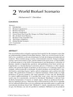
7
Acquisition and Interpretation of Water-Level Data
Matthew G. Dalton, Brent E. Huntsman, and Ken Bradbury
CONTENTS
Introduction . . . . . . . . . . . . . . . . . . . . . . . . . . . . . . . . . . . . . . . . . . . . . . . . . . . . . . . 174
Importance of Water-Level Data . . . . . . . . . . . . . . . . . . . . . . . . . . . . . . . . . . . . . . 174
Water-Level and Hydraulic-Head Relationships . . . . . . . . . . . . . . . . . . . . . . . . . . 174
Hydraulic Media and Aquifer Systems . . . . . . . . . . . . . . . . . . . . . . . . . . . . . . . . . 175
Design Features for Water-Level Monitoring Systems . . . . . . . . . . . . . . . . . . . . . . . . 176
Piezometers or Wells? . . . . . . . . . . . . . . . . . . . . . . . . . . . . . . . . . . . . . . . . . . . . . . 176
Approach to System Design . . . . . . . . . . . . . . . . . . . . . . . . . . . . . . . . . . . . . . . . . 177
Number and Placement of Wells . . . . . . . . . . . . . . . . . . . . . . . . . . . . . . . . . . . . . . 178
Screen Depth and Length . . . . . . . . . . . . . . . . . . . . . . . . . . . . . . . . . . . . . . . . . . . 178
Construction Features . . . . . . . . . . . . . . . . . . . . . . . . . . . . . . . . . . . . . . . . . . . . . . 180
Water-Level Measurement Precision and Intervals . . . . . . . . . . . . . . . . . . . . . . . . 181
Reporting of Data . . . . . . . . . . . . . . . . . . . . . . . . . . . . . . . . . . . . . . . . . . . . . . . . . 182
Water-Level Data Acquisition . . . . . . . . . . . . . . . . . . . . . . . . . . . . . . . . . . . . . . . . . . 182
Manual Measurements in Nonflowing Wells . . . . . . . . . . . . . . . . . . . . . . . . . . . . . 183
Wetted Chalked Tape Method . . . . . . . . . . . . . . . . . . . . . . . . . . . . . . . . . . . . . . 184
Air-Line Submergence Method . . . . . . . . . . . . . . . . . . . . . . . . . . . . . . . . . . . . . 184
Electrical Methods . . . . . . . . . . . . . . . . . . . . . . . . . . . . . . . . . . . . . . . . . . . . . . . 185
Pressure Transducer Methods . . . . . . . . . . . . . . . . . . . . . . . . . . . . . . . . . . . . . . 186
Float Method . . . . . . . . . . . . . . . . . . . . . . . . . . . . . . . . . . . . . . . . . . . . . . . . . . . 187
Sonic or Audible Methods . . . . . . . . . . . . . . . . . . . . . . . . . . . . . . . . . . . . . . . . . 187
Popper . . . . . . . . . . . . . . . . . . . . . . . . . . . . . . . . . . . . . . . . . . . . . . . . . . . . . . 187
Acoustic Probe . . . . . . . . . . . . . . . . . . . . . . . . . . . . . . . . . . . . . . . . . . . . . . . . 187
Ultrasonic Methods . . . . . . . . . . . . . . . . . . . . . . . . . . . . . . . . . . . . . . . . . . . . . . 188
Radar Methods . . . . . . . . . . . . . . . . . . . . . . . . . . . . . . . . . . . . . . . . . . . . . . . . . 188
Laser Methods . . . . . . . . . . . . . . . . . . . . . . . . . . . . . . . . . . . . . . . . . . . . . . . . . . 188
Manual Measurements in Flowing Wells . . . . . . . . . . . . . . . . . . . . . . . . . . . . . . . . 189
Casing Extension . . . . . . . . . . . . . . . . . . . . . . . . . . . . . . . . . . . . . . . . . . . . . . . . 189

Manometers and Pressure Gages . . . . . . . . . . . . . . . . . . . . . . . . . . . . . . . . . . . . 189
Pressure Transducers . . . . . . . . . . . . . . . . . . . . . . . . . . . . . . . . . . . . . . . . . . . . . 189
Applications and Limitations of Manual Methods . . . . . . . . . . . . . . . . . . . . . . . . 190
Continuous Measurements of Ground-Water Levels . . . . . . . . . . . . . . . . . . . . . . . 190
Methods of Continuous Measurement . . . . . . . . . . . . . . . . . . . . . . . . . . . . . . . . . 190
Mechanical: Float Recorder Systems . . . . . . . . . . . . . . . . . . . . . . . . . . . . . . . . . 190
Electromechanical: Iterative Conductance Probes (Dippers) . . . . . . . . . . . . . . . . 191
Data Loggers . . . . . . . . . . . . . . . . . . . . . . . . . . . . . . . . . . . . . . . . . . . . . . . . . . . 191
Analysis, Interpretation, and Presentation of Water-Level Data . . . . . . . . . . . . . . . . 192
173
© 2007 by Taylor & Francis Group, LLC
Recharge and Discharge Conditions . . . . . . . . . . . . . . . . . . . . . . . . . . . . . . . . . . . 193
Approach to Interpreting Water-Level Data . . . . . . . . . . . . . . . . . . . . . . . . . . . . . 194
Transient Effects . . . . . . . . . . . . . . . . . . . . . . . . . . . . . . . . . . . . . . . . . . . . . . . . . . 197
Contouring of Water-Level Elevation Data . . . . . . . . . . . . . . . . . . . . . . . . . . . . . . 200
References . . . . . . . . . . . . . . . . . . . . . . . . . . . . . . . . . . . . . . . . . . . . . . . . . . . . . . . . 200
Introduction
Importance of Water-Level Data
The acquisition and interpretation of water-level data are essential parts of any
environmental site characterization or ground-water monitoring program. When trans-
lated into values of hydraulic head, water-level measurements are used to determine the
distribution of hydraulic head in one or more formations. This information is used, in
turn, to assess ground-water flow velocities and directions within a three-dimensional
framework. When referenced to changes in time, water-level measurements can reveal
changes in ground-water flow regimes brought about by natural or human influences.
When measured as part of an in situ well or aquifer pumping test, water levels provide
information needed to evaluate the hydraulic properties of ground-water systems.
Water-Level and Hydraulic-Head Relationships
Hydraulic head is the driving force for ground-water movement and varies both spatially
and temporally. A piezometer is a monitoring device specifically designed to measure

hydraulic head at a discrete point in a ground-water system. Figure 7.1 shows water-level
and hydraulic-head relationships at a simple vertical standpipe piezometer (A). The
piezometer consists of a hollow vertical casing with a short screen open at point P. The
piezometer measures total hydraulic head at point P. Total hydraulic head (h
t
) has two
components — elevation head (h
e
) and pressure head (h
p
).
FIGURE 7.1
Hydraulic-head relationship at a field piezometer. (Adapted from Freeze and Cherry (1979). With permission.)
174 The Essential Handbook of Ground-Water Sampling
© 2007 by Taylor & Francis Group, LLC
Elevation head (h
e
) refers to the potential energy that ground water possesses by virtue of
its elevation above a reference datum. Elevation head is caused by the gravitational
attraction between water and earth. In Figure 7.1, the elevation head (h
e
) at point P is 7 m.
Pressure head (h
e
) refers to the force exerted on water at the measuring point by the
height of the static fluid column above it (in this discussion, atmospheric pressure is
neglected). In Figure 7.1, the pressure head (h
p
) at point P is 6 m. Note that h
p

is measured
inside the piezometer and corresponds to the distance between point P and the water
level in the piezometer.
Total hydraulic head (h
t
) is the sum of elevation head (h
e
) and pressure head (h
p
). The
total hydraulic head at point P in Figure 7.1 is 7 '6 0 13 m relative to the datum.
The water level in piezometer A is lower than the water level (at the water table)
measured in piezometer B. The difference in elevation between the water-table piezo-
meter (B) and the water level in the deeper piezometer (A) corresponds to the hydraulic
gradient between the two piezometers. In this case, there is a downward vertical gradient
because total hydraulic head decreases from top to bottom.
Hydraulic Media and Aquifer Systems
The ‘‘classic’’ definition of an aquifer as ‘‘a water-bearing layer of geologic material, which
will yield water in a usable quantity to a well or spring’’ (Heath, 1983) was developed to
address water-supply issues, but it is less useful for describing materials in terms of modern
ground-water monitoring. Today, ground-water monitoring (including well installation,
water-level measurement, and water-quality assessment) occurs in hydrogeologic media
ranging from very low hydraulic conductivity shales, clays, and granites to very high
hydraulic conductivity sands and gravels. The term aquifer (in ground-water monitoring) is
used as a relative term to describe any and all of these materials in various settings.
Aquifers are also generally classified based on where a water level lies with respect to
the top of the geologic unit. Figure 7.2 shows an example of layered hydrogeologic media
forming both confined and unconfined aquifers. The confined aquifer is a relatively high
hydraulic conductivity unit, bounded on its upper surface by a relatively lower hydraulic
conductivity layer. Hydraulic head in the confined aquifer is described by a potentio-

metric surface, which is an imaginary surface representing the distribution of total
hydraulic head (h
t
) in the aquifer and which is higher in elevation than the physical top of
the aquifer.
The sand layer in the upper part of Figure 7.2 contains an unconfined aquifer, which
has the water table as its upper boundary. The water table is a surface corresponding to
FIGURE 7.2
Unconfined aquifer and its water table; confined aquifer and its potentiometric surface. (Adapted from Freeze
and Cherry [1979]. With permission.)
Acquisition and Interpretation of Water-Level Data 175
© 2007 by Taylor & Francis Group, LLC
the top of the unconfined aquifer where total hydraulic head is zero relative to
atmospheric pressure or the hydrostatic pressure is equal to the atmospheric pressure.
Notice that water levels in the piezometers in Figure 7.2 vary with the depth and
position of the piezometer. This variation corresponds to the variation of total hydraulic
head throughout the saturated system. Hydraulic head often varies greatly in three
dimensions over small areas. Thus, the design and placement of water-level monitoring
equipment is critical for a proper understanding of the ground-water system.
Design Features for Water-Level Monitoring Systems
An important use of ground-water level (hydraulic head) data from wells or piezometers
is assessment of ground-water flow directions and hydraulic gradients. The design of
ground-water monitoring systems must usually consider requirements for both water-
level monitoring and ground-water sampling. In many cases, both needs can be
accommodated with one set of wells and without installing separate systems. However,
to collect acceptable water-level data, certain requirements need to be met, which may not
always be consistent with the requirements for collecting ground-water samples. For
example, additional wells may be required to fully assess the configuration of a water
table or potentiometric surface over and above the wells that might be required to collect
ground-water samples. Conversely, the design of wells to collect ground-water samples

may differ from wells that are used solely to collect ground-water level data.
Water-level monitoring data are generally collected during two phases of a monitoring
program. The initial phase is when the site to be monitored is being characterized to
provide data to design a monitoring system. The second phase is when water-level data
are being collected as part of the actual monitoring program to assess whether changes in
ground-water flow directions are occurring and to confirm that wells used to provide
ground-water samples are properly located (i.e., hydraulically upgradient and down-
gradient of a facility that requires monitoring). The latter data also provide a basis to
determine the cause of flow-direction changes and to assess whether the monitoring
system needs to be reconfigured to account for these changes.
To design a water-level monitoring system, a detailed understanding of the site geology
is necessary. The site geology is the physical structure in which ground-water flows and,
as such, has a profound influence on water-level data. It is very important that reliable
geologic data be collected so that the water-level monitoring system can be properly
designed and the water-level data can be accurately interpreted.
Sites at which there is a high degree of geologic variation require more extensive (and
costly) water-level monitoring systems than sites that are comparatively more homo-
geneous in nature. The degree of geologic complexity is often not known or appreciated
during the early phases of a site-characterization program, and it may require several
stages of drilling, well installation, water-level measurement, and analysis of hydro-
geologic data before the required level of understanding is achieved.
Piezometers or Wells?
Ground-water level measurements are typically made in piezometers or wells. Most
ground-water monitoring systems associated with assessing ground-water quality are
composed of wells rather than piezometers.
176 The Essential Handbook of Ground-Water Sampling
© 2007 by Taylor & Francis Group, LLC
Piezometers are specialized monitoring installations; the primary purpose of which is
the measurement of hydraulic head. Generally, these installations are relatively small in
diameter (less than 1 in. in diameter if a well casing is used), or in some applications, it

may not include a well casing and just consist of tubes or electrical wires connected to
pressure or electrical transducers. Piezometers are not typically designed to obtain
ground-water samples for chemical analysis, although the term piezometer has been
applied to pressure measuring devices which have been modified to collect ground-water
samples (Maslansky et al., 1987). Piezometers have traditionally had the greatest
application in geotechnical engineering for measuring hydraulic heads in dams and
embankments.
Wells are normally the primary devices in which water levels are measured as part of a
monitoring system. They differ from piezometers in that they are typically designed so
ground-water samples can be collected. To accommodate this objective, wells are larger in
diameter than piezometers (usually larger than 1.5 in. in diameter), although sampling
devices have been developed, which allow ground-water samples to be obtained from
small-diameter wells (see Chapter 3).
Approach to System Design
Design of a water-level monitoring system should begin with a thorough review of
available existing data. This review should be directed toward developing a conceptual
model of the site geologic and hydrologic conditions. The conceptual model of the
hydrogeologic system is used to determine the locations of an initial array of wells.
Tentative decisions regarding drilling depths and the zone or zones to be screened should
also be made using existing data. Existing wells may be incorporated into the array if
suitable information regarding well construction details is available. Boring and well
construction logs, surficial geologic and topographic maps, drainage features, cultural
features (e.g., well fields, irrigation, and buried water pipes), and rainfall and recharge
patterns (both natural and man-induced) are several of the major factors that need to be
assessed as completely as possible.
The available data should be reviewed to identify:
. The depth and characteristics of relatively high hydraulic conductivity geologic
materials (aquifers) and low hydraulic conductivity confining beds that may be
present beneath a site
. Depth to the water table and the likelihood of encountering perched or

intermittently saturated zones above the water table
. Probable ground-water flow directions
. Presence of vertical hydraulic gradients
. Features that might cause ground-water levels to fluctuate, such as well-field
pumping, fluctuating river stages, unlined ditches or impoundments, or tides
. Probable frequency of fluctuation
. Existing wells that may be incorporated into the water-level monitoring program
The practical limitations of where wells can be located on a site should not be
overlooked during this phase of the system design. Wells can be located almost anywhere
on some sites; however, on other sites, buildings, buried utilities, and other site features
can impose limitations on siting wells.
Acquisition and Interpretation of Water-Level Data 177
© 2007 by Taylor & Francis Group, LLC
Number and Placement of Wells
The number of wells required to assess ground-water flow directions beneath a site is
dependent on the size and complexity of the site conditions. Simple and smaller sites
require fewer wells than larger or more hydrogeologically complex sites.
Many sites have more than one saturated zone of interest in which ground-water flow
directions need to be assessed. High hydraulic conductivity zones may be separated by
lower hydraulic conductivity zones. In these cases, several wells screened at different
depths may be required at several locations to adequately assess flow directions in, and
between, each of the saturated zones of interest.
The minimum number of wells required to estimate a ground-water flow direction
within a zone is three (Todd, 1980; Driscoll, 1986). However, the use of just three wells is
only appropriate for relatively small sites with very simple geology, where the
configuration of the water table or potentiometric surface is essentially planar in nature,
as shown in Figure 7.3.
Generally, conditions beneath most sites require more than three wells. Lateral
variations in the hydraulic conductivity of subsurface materials, localized recharge
patterns, drainage channels, and other factors can cause the potentiometric or water-table

surface to be nonplanar.
On large or more geologically complex sites, an initial grid of six to nine wells is usually
sufficient to provide a preliminary indication of ground-water flow directions within a
target ground-water zone. Such a configuration will generally allow the complexities in
the water table or potentiometric surface to be identified. After an initial set of data is
collected and analyzed, the need for and placement of additional monitoring installations
can be assessed to fill in data gaps or to further refine the assessment of the
potentiometric or water-table surface.
Figure 7.4 shows a site at which leakage from a buried pipe has caused a ground-water
mound to form. In this situation, a three-well array would not provide sufficient data to
detect the presence of the mound and could result in a faulty assessment of the
groundwater flow direction beneath the site.
Screen Depth and Length
After well locations are established, well screen depths and lengths should be chosen.
Screen depths are generally determined during the drilling operation after a geologic log
FIGURE 7.3
Assessing ground-water flow directions at a small site with a planar water-table surface.
178 The Essential Handbook of Ground-Water Sampling
© 2007 by Taylor & Francis Group, LLC
has been prepared, depending on the amount and quality of the data available prior to
drilling.
Wells used to assess flow directions within a zone are usually screened within that zone
at similar elevations. Highly layered units may require screens in each depth zone that is
isolated by lower hydraulic conductivity layers (Figure 7.5a). Where the units are
dipping, it is generally more important to place the screens in the same zone even if the
screens are not placed at similar elevations (Figure 7.5b).
Similar well-screen lengths should be used and the screen (and filter pack) should be
placed entirely within the zone to be monitored. This will allow field personnel to obtain
a water level that is representative of the zone being monitored and will minimize the
possibility of allowing contaminants, if present, to migrate between zones screened by the

well. If the well screen is open to several zones, then a composite or average water level
will be measured, which will not be representative of any single zone, and will add to the
difficulty in interpreting the water-level data. Typical commercially available well screens
are 5 or 10 ft long, although it is possible to construct wells with longer or shorter screens,
to meet specific project objectives.
If multiple saturated zones are present beneath a site, it is generally necessary to install
either several wells screened at different depths at a single location or a multilevel
monitoring system. Such installations allow the assessment of both horizontal and
vertical hydraulic gradients. If few reliable data are available for a site, it is desirable that
the initial hydrologic characterization starts with the uppermost zone of interest. During
this initial work, a limited number of deeper installations can be installed to provide data
FIGURE 7.4
Estimation of ground-water flow directions with a three-well and a nine-well array.
Acquisition and Interpretation of Water-Level Data 179
© 2007 by Taylor & Francis Group, LLC
to assess the need for additional deeper installations. In situations in which contamina-
tion is present in a shallow aquifer, extreme care must be exercised with regard to
installing deeper wells, to prevent the possible downward movement of contamination
into deeper zones.
Construction Features
Water-level monitoring points can be installed using a variety of methods and configura-
tions (Figure 7.6). Typically, the installations are constructed in drilled boreholes, although
FIGURE 7.5
Well screen placement in horizontal and dipping strata.
FIGURE 7.6
Typical monitoring well installation configurations.
180 The Essential Handbook of Ground-Water Sampling
© 2007 by Taylor & Francis Group, LLC
driven well points can be used to provide water-level data in shallow, unconfined
saturated zones.

At locations where multiple zones are to be monitored, single or multiple installations
in the same borehole or multilevel systems can be used. If a single well is installed in a
borehole, several boreholes will be necessary to monitor multiple zones.
A single installation in a single borehole is often preferred because it is easier to install a
reliable annular seal above the well screen when only one well is completed in a borehole.
An annular seal is necessary to ensure that the water-level data are representative of the
zone being monitored and to ensure that contaminants do not move between zones
within the borehole. In many situations, especially if a hollow-stem auger is being used to
install the well, the cost of installing single installations is only marginally higher than
multiple installations in a single borehole.
Multiple installations in a single borehole have been installed successfully as long as an
adequate borehole or drill casing diameter is used and care is taken in installing the wells.
Installing two 2 in. diameter wells per borehole should be feasible within 6 to 8 in.
diameter boreholes or drill casings. While multiple installations in the same borehole may
be technically feasible, some local well-drilling regulations may preclude or restrict such
installations.
Water-Level Measurement Precision and Intervals
Wells should be accurately located horizontally and vertically, although horizontal
surveying is not always required, depending on the size of the site and available base
maps. The precision of the horizontal locations is generally not as important as the
precision of the elevation survey and water-level measurements.
The top of the well casing (or other convenient water-level measuring point) should be
surveyed to a common datum (usually National Geodetic Vertical Datum or NGVD) so
that water-level measurements can be converted to water-level elevations. The reference
point for water-level measurements should be clearly marked at a convenient location on
each well casing. This will facilitate reducing measurement error.
The precision of the elevation survey and water-level measurements depends on the
slope of the potentiometric or water-table surface and the distance between wells. Greater
precision is required at sites where the surface is gradual or the wells are close together.
Generally, reference point elevations should be surveyed and water levels measured with

a precision ranging between 90.1 and 90.01 ft.
For example, if water-level fluctuations are occurring over a short period of time, it may
be more important to obtain a set of less precise measurements in a short period of time
rather than a very precise set of measurements over a longer period of time. In such cases,
measurements made to 0.1 ft may be appropriate. In contrast, if the slope of the
potentiometric surface or water-table surface is very gradual, more precise elevation
control and water-level measurements may be required.
Current environmental regulations generally require that water levels be monitored
and reported on a quarterly basis. A quarterly monitoring schedule may be appropriate
for sites at which water levels fluctuate only in response to seasonal conditions, such as
precipitation or irrigation recharge. However, water levels at many sites respond not only
to seasonal factors but also to factors of shorter duration or greater frequency. These
factors may include fluctuations caused by tides in coastal areas, changes in river stage,
and daily well pumping, among others. Separate zones may also respond differently to
the cause of the fluctuations.
Acquisition and Interpretation of Water-Level Data 181
© 2007 by Taylor & Francis Group, LLC
During site-characterization activities, factors that may cause water levels to fluctuate
need to be assessed and their importance evaluated with respect to two issues:
. The time in which a set of water-level measurements needs to be obtained
. How the flow directions may change as the water levels fluctuate
With the advent of computer technology, our ability to analyze complex systems at a
reasonable cost has increased dramatically. Microprocessors connected to transducers
allow the collection and analysis of water-level data over extended periods of time. To
determine a site-specific monitoring interval, continuous monitoring can be economically
accomplished in selected wells screened at different depths and at varying distances from
the cause of the fluctuation. These data can then be used to determine the time frame and
intervals in which to obtain water-level measurements and to determine how the various
zones beneath the site respond to the cause of the fluctuation.
The period in which the continuous monitoring should be conducted depends on the

frequency and duration of the fluctuations. If possible, monitoring should be conducted
at times of representative fluctuation. For example, on sites affected by tides, monitoring
over several tidal cycles during relatively high and low tides may be warranted.
Reporting of Data
Interpretation of water-level data requires that information be available about the
monitoring installations and the conditions in which the water-level measurements
were made. This information includes:
. Monitoring installations
a. Geologic sequence
b. Well construction features, especially screen and sand pack length, and
geologic strata in which the screen is situated
c. Depth and elevation of the top and bottom of the screen and sand pack
d. Measuring point location and elevation
e. Casing stickup above ground surface
. Water-level data
a. Date and time of measurement
b. Method used to obtain the measurement
c. Other conditions in the area that might be affecting the water-level data, such
as tidal or river stage, well pumping, storm events, etc.
Water-Level Data Acquisition
For many purposes in ground-water investigations, the accurate determination of water
levels in wells or piezometers is paramount. Without accurate measurements, it is not
possible to interpret the data to assess conditions such as ground-water flow directions,
ground-water flow velocities, seasonal variations in water levels, aquifer hydraulic
conductivity, and other important features.
182 The Essential Handbook of Ground-Water Sampling
© 2007 by Taylor & Francis Group, LLC
Depending upon the ultimate use of the water-level data, the methods and instruments
used to collect and record changes in ground-water levels may vary substantially. Water-
level data acquisition techniques are divided into two major categories for discussion

purposes: manual measurements or typically nonrecording methods and continuous
measurements using instruments that provide a record. Although not exhaustive, the
following discussion describes techniques most frequently used by the practicing
hydrogeologist. These methods are summarized in Table 7.1.
Manual Measurements in Nonflowing Wells
Accurate manual measurements of water levels in wells and piezometers should be a core
skill for any practicing hydrologist, hydrogeologist, ground-water scientist, or technician.
Regardless of the method used, repeated measurements of water levels in wells made
within a few minutes and within 200 ft of the top of casing should agree within 0.01 or
0.02 ft. As a standard of good practice, Thornhill (1989) suggests that anyone obtaining a
water-level measurement in a well should take at least two readings. If they differ by
more than 0.02 ft, then continue to measure until the reason for the lack of agreement is
determined or until the results are shown to be stable.
TABLE 7.1
Summary of Methods for Manual Measurement of Well-Water Levels in Nonflowing and
Flowing Wells
Measurement Method Measurement Accuracy (ft)
Major Interference
or Disadvantage
Nonflowing Wells
Wetted chalked tape 0.01 Cascading water or casing wall
water and chalk in water
Air line 0.01Á
/0.25 Air line or fitting leaks; gage
inaccuracies and air source
Electrical probes 0.02Á
/0.1 Cable wear; hydrocarbons on water
surface and turbulence
Transducer 0.01Á
/0.1 Temperature changes; electronic

drift; blocked capillary
Float 0.02Á
/0.5 Float or cable drag; float
size and lag
Popper 0.1 Well noise; well pipes and pumps;
well depth
Acoustic probe 0.02 Cascading water; hydrocarbon on
water surface
Ultrasonic 0.02Á
/2.4 Temperature changes; well pipes
and pumps; casing joints
Radar 0.01Á
/0.02 Temperature; humidity; well pipes
and pumps, small wells
Laser 0.01 Nonstraight wells; beam penetration
through water
Flowing Wells
Casing extensions 0.1 Limited range; awkward
to implement
Manometer and pressure gage 0.1 Gage inaccuracies; calibration
required
Transducers 0.02Á
/0.1 Temperature changes;
electronic drift
Acquisition and Interpretation of Water-Level Data 183
© 2007 by Taylor & Francis Group, LLC
Wetted Chalked Tape Method
Although less commonly utilized in today’s hydrologic assessments, one of the most
accurate techniques used to manually measure ground-water levels is the wetted chalked
tape method (ASTM D 4750; ASTM, 2006a). The equipment needed to make a

measurement using this method consists of a standard steel surveyor’s tape, a block of
carpenter’s chalk, and a slender lead or stainless-steel weight. Steel tapes and hand reels
are commercially available in lengths up to 1000 ft. It is recommended, however, that
shorter standard lengths (100, 200, 300, and 500 ft) be used because of weight and cost.
Steel-tape markings are usually divided only into tenths of feet or inches and fractions of
an inch. Interpolation to the nearest 0.01 ft is possible.
The weight is attached to the steel tape end clip with sufficient wire for support, but not
enough to be stronger than the tape. This allows the tape to be pulled free if the weight
become snagged on something in the well. The bottom 2 or 3 ft of the tape is coated with
carpenter’s chalk. A water-level measurement is made by lowering the tape slowly into
the well, about 1 or 2 ft into the water. It is convenient to lower the tape into the water a
sufficient distance to allow the tape to read an even foot mark at the top of the well casing
or the reference measuring point at the surface. The water-level measurement is
calculated by subtracting the submerged distance, as indicated by the absence of change
in chalk color, from the reference point at the top of the well.
The practical limit of measurement precision for this method is 90.01 ft (U.S.
Geological Survey, 1980). Coefficients of stretch and temperature expansion of the steel
tape become a concern when water-level measurements are made in wells that have
higher temperatures or at depths greater than 1000 ft (Garber and Koopman, 1968). For
most ground-water investigations, corrections for these errors are not necessary.
A disadvantage of using the wetted chalked tape method is that if the approximate
depth to water is unknown, too short or too long a length of chalked tape may be lowered
into the well, thereby necessitating a number of attempts. In addition, water condensed
on the side of the casing, or cascading water, may wet the tape above the actual water
level and result in errors in measurement (Everett, 1980). When compared with other
manual measurement techniques, this method is more time consuming. Proficiency in
obtaining water levels with a wetted chalked tape requires practice. In addition, the
introduction of chalk into a well that is used to obtain water-quality samples is
discouraged.
Air-Line Submergence Method

The air-line submergence method, although less precise than other manual water-level
measurement methods, continues to be a preferred technique in wells that are being
pumped. To make an air-line measurement of water level in a well, a straight, small-
diameter tube of accurately known length is installed in the well. This tube, usually
0.375 in. or less in diameter, can be made of plastic, copper, or steel. The air line and all
connections must be air tight, without bends or kinks, and installed to several feet below
the lowest anticipated water level. A pressure gage (preferably calibrated in feet of water),
along with a fitting for an air source, is attached to this line. In deep wells or where
multiple water-level measurements are needed, a small air compressor is useful. In
shallow wells, a hand-operated air pump is typically used.
A water-level measurement is made when air is pumped into the small tube and the
pressure is monitored. Air pressure will continue to increase until it expels all water from
the line. Air pressure, which is determined when the pressure gage stabilizes, is used to
calculate the height of the water in the tube. If the pressure gage is calibrated in pounds
per square inch (psi), a conversion is made to feet by multiplying the psi reading by 2.31.
184 The Essential Handbook of Ground-Water Sampling
© 2007 by Taylor & Francis Group, LLC
The actual water level in the well is determined by subtracting the calculated distance
from the air line’s length. According to Driscoll (1986), the dependability of measure-
ments made by the air-line method varies with the accuracy of the pressure gage and the
care used in determining the initial pressure reading. Depth to water can usually be
determined to within 0.25 ft of the true water level. Garber and Koopman (1968) have also
shown that the precision of the measurement is mainly dependent upon the accuracy of
the pressure gage. They state that even with gages having gradations as small as 0.1 psi,
the maximum possible resolution would be 0.23 ft. Digital quartz pressure transducers
and specialized data loggers have been tested as replacements for standard pressure
gages. Water levels from 0 to 50 ft have been measured with an accuracy of better than
0.01 ft (Paroscientific, Inc., 2002). However, these precision pressure measurement
systems are designed for more permanent installations, not for portable applications.
Unless the air-line method is used in wells of substantial depth, corrections for thermal

expansion, hysteresis, fluid density, and barometric pressure are not necessary.
Electrical Methods
Currently, the most favored technique for manual water-level measurement is the use of
an electrical probe. The most widely used instrument of this type is one that operates on
the principle that a circuit is completed when two electrodes come in contact with the
water surface in the well, which is conductive. Other instruments rely on physical
characteristics such as resistance, capacitance, or self-potential to produce a signal. Many
of these instruments employ a two-wire conductor that is marked every foot, with minor
interval markings of 0.01 ft. Some instruments use vinyl-, epoxy-, or Teflon-clad steel
tapes as an insulated electrode and the well casing or grounding wire as the other
electrode. Because of weight and the amount of potential cable stretch, most commercial
electrical probes are designed for water-level measurements within several hundred feet
of the top of casing.
Water-level probes that use self-potential typically have one electrode made of
magnesium and the other made of brass or steel. When the probe comes into contact
with water, a potential between the two dissimilar metals is measured at the surface on a
voltmeter (generally in millivolts).
If a battery is added to the circuit, the two electrodes may be of the same material,
usually brass, lead, or ferrous alloy. When the electrodes come into contact with the water
surface, the water conducts the current and a meter, light, or buzzer is activated at the
ground surface.
The principles of capacitance and inductance have been used by the U.S. Geological
Survey to detect water surfaces (Garber and Koopman, 1968). These are basically
specialty instruments and few are available commercially for common water-level
measurements. However, some units that employ capacitance or inductance are used
for detection of water levels and hydrocarbons in wells. These units have the same
apparent accuracy and precision as other electrical probes because the sensing elements
are suspended in the well via multiwire conductors.
Errors in water-level measurements using electrical probes result from changes in the
cable length and diameter as a function of use, depth, and temperature. After repeated

use, the markings on the drop line often have a tendency to become loose and slide (if
banded) or become illegible from wear (if embossed). Shallow measurements made with
well-maintained electrical probes are typically reproducible to within 90.02 ft. Because of
kinks in the cable and less than vertical suspension in a well, Barcelona et al. (1985) stated
that the accuracy of electrical probes is about 0.1 ft. Plazak (1994) showed that even the
Acquisition and Interpretation of Water-Level Data 185
© 2007 by Taylor & Francis Group, LLC
same make and model of electrical probes may vary 90.01 to 90.11 ft in precision and
accuracy, depending on the depth of the water-level measurement.
A disadvantage inherent in most electrical probe instruments is that if substantial
amounts of oil or other nonconductive materials (i.e., oils) are floating upon the water
surface, contact cannot be reliably made. This is a major concern in ground-water
investigations involving petroleum hydrocarbon releases. Special sensing probes utilizing
an optical or infrared sensor in conjunction with electrical conductivity are commercially
available to measure the hydrocarbon-water interface. Because this type of sensing probe
is also suspended from multiconductor wire, the same errors as previously discussed for
electrical probes apply.
Pressure Transducer Methods
With the advent of reliable silicon-based strain gage pressure sensors and vibrating-wire
transducers, a unique type of instrument is being commercially marketed for measuring
changes in water levels. These transducers contain a 4Á20 mA current transmitter and a
strain gage sensor or a vibrating wire in an electromagnetic coil with frequency
measurement circuitry. The current transmitter circuitry in both types of transducers
prevents measurement sensitivity from being affected by cable length. Because all
sensitive electronics are in the transducer and submerged in a constant temperature
environment (the well water), errors due to temperature fluctuations are negligible (In
Situ, Inc., 1983; Zarriello, 1995). The simultaneous measurement of temperature and water
level is becoming a standard feature for most of the transducers used in hydrogeologic
studies.
Many transducers used for measuring ground-water levels have a small capillary tube

shielded in the support cable leading from one side of a differential pressure sensor. This
tube is vented to the atmosphere, which provides automatic compensation of barometric
pressure. Care must be taken when working with transducer cables that contain
capillaries to avoid kinking, crushing, or allowing condensate to form in the vent tube.
Blocked vent tubes may result in erroneous water-level measurements. A signal
conditioning unit and a power source are required ancillary equipment to make a
water-level measurement.
To avoid the need for electrical cables to transmit signals from the transducer to the
data storage unit, some manufacturers have totally sealed the data logger, battery,
pressure transducer, and temperature sensor in a small stainless-steel case for total
submersion in a well. Communication with the data logger is established via an infrared
optical port, either with a cradle component or through extension cables connected to a
host computer. These units use an absolute pressure sensor to avoid the need for a vent
tube to the surface. However, all water-level readings obtained by this type of monitor
will require subsequent corrections for barometric pressure changes (Solinst Ltd., 2001).
For a discrete water-level measurement, the transducer is lowered a known distance into
the well and allowed to equilibrate to the fluid temperature. The distance of submergence
of the transducer is read on the signal conditioning unit and is subtracted from the known
cable length referenced at the top of the well.
This technique is easily adaptable to continuous monitoring. It also offers several
advantages in ease of accurate measurement in both pumping wells and wells with
cascading water. Sources of error in this type of instrument include the electronics
(linearity, accuracy, temperature coefficient, etc.), temperature changes, and inappropriate
application (i.e., range and material of construction) of a transducer in a given medium
(Sheingold, 1980; Zarriello, 1995). Because of the sensitive electronics, rough handling of
the transducers in the field or in storage should be avoided.
186 The Essential Handbook of Ground-Water Sampling
© 2007 by Taylor & Francis Group, LLC
The accuracy of water-level transducers is dependent upon the type and range
(sensitivity) of the device used. Most transducers are rated in terms of a percent of their

full-scale capability. For example, a 0 to 5 psi tranducer rated at 0.01) will provide
measurements to the nearest 0.01 ft. In contrast, a 0 to 25 psi transducer rated at 0.01)
will provide measurements to the nearest 0.05 ft (Barcelona et al., 1985). Standard
practices for the static calibration of electronic transducers used for obtaining field
pressure measurements have been developed and should be used to document the
accuracy of the instrumentation system (ASTM D 5720; ASTM, 2006b). These calibration
procedures are typically included in the standard operating procedures prepared for any
large-scale hydrogeologic investigation in which electronic pressure transducers are used.
Float Method
As the name implies, a float is attached to a length of steel tape and suspended over a
pulley into the well. At the opposite end of the steel tape, a counterweight is attached. The
depth to water is read directly from the steel tape at a known reference point at the top of
the casing.
To obtain an accurate measurement using this technique, the absolute length of the float
assembly must be measured and subtracted from the steel-tape measurement. For greater
accuracy, the total amount of float submergence should be calculated and a correction
factor applied. This becomes more critical with smaller diameter floats (Leupold and
Stevens, Inc., 1978). This method is used principally to obtain continuous water-level
measurements. The accuracy and errors in float-operated devices will be discussed in
greater detail in the following section.
Sonic or Audible Methods
Virtually every practicing hydrogeologist has (but should not have) dropped a rock down
a well, at one time or another, to determine whether water is present and to estimate the
depth to water. Stewart (1970) investigated and developed a technique to determine the
depth to water by timing the fall of a BB (air rifle shot) or a glass marble and by recording
the time of the return sound of impact. This sonic technique will not be discussed here in
detail because of the rather large range of error in measurement (95 ft), but interested
readers are referred to Stewart (1970). Other sonic methods are described subsequently.
Popper
The most simplistic device used to audibly determine the depth to water in a well casing is

a popper (also called a plopper). This is a metal cylinder from 1 to 1.5 in. in diameter and
generally 2 to 6 in. in length, with a concave bottom. The popper is attached to a steel tape
and lowered to within a few inches of the water surface in the well. By repeatedly dropping
the popper onto the water surface and noting the tape reading at which a distinctive ‘‘pop’’
is heard, the depth to water is determined (U.S. Bureau of Reclamation, 2001).
Because of noise and the lack of clearance, the use of poppers in pumping wells is
limited. The accuracy of water-level measurements made by this technique is highly
dependent upon the skill of the measurer and the depth of the well. Determination of the
water level to within 0.02 ft is usually the detection limit of this procedure.
Acoustic Probe
A unique adaptation of the popper principle was developed by Schrale and Brandwyk
(1979), with the construction of an acoustic probe. This electronic device is attached to a
steel tape and lowered into the well until an audible sound is emitted from a battery-
powered transducer contained in the probe. The electric circuit is completed when the
Acquisition and Interpretation of Water-Level Data 187
© 2007 by Taylor & Francis Group, LLC
two electrodes placed in the bottom of the probe come in contact with the water level in
the well. As with the previously discussed electrical methods, problems with measure-
ments can occur when hydrocarbons are present or if the well has cascading water.
According to the developers of this instrument, a water-level determination is possible to
within 90.02 ft.
Ultrasonic Methods
Instruments that measure the arrival time of a reflected transmitted sonic or ultrasonic
wave pulse are becoming more common in the measurement of water levels. These
instruments electronically determine the amount of time it takes for a sound wave to travel
down the well casing, reflect off the water surface, and return to the surface. Because the
electronic circuitry typically uses microprocessors, this signal is transmitted, received, and
averaged many times a second. The microprocessor also calculates the depth to water and
displays it in various units. Several of the commercially available instruments simply rest
on top of the well casing with nothing being lowered into the well. Rapid determination of

water depths in deep wells is a distinct advantage of this technique.
The presence of hydrocarbons on the water surface usually has no effect on the
measurement. Accuracy can be limited by change of temperature in the path of the sound
wave and other reflective surfaces in the well (i.e., pipes, casing burrs, pumps, samplers,
crooked casing, etc.). Large variations in humidity will also effect readings. Most
commercially available hand-held units can measure the depth to water within 0.1 ft if
the well’s temperature gradient is uniform. Usually, the greater the depth to water, the
less accurate the measurement. One manufacturer reports a 90.2) accuracy over a range
of 25 to 1200 ft. Specialized installations, however, have repeatedly provided water-level
measurements accurate to within 90.02 ft (Alderman, 1986).
Radar Methods
Similar to the ultrasonic measurement instrumentation, radar-based portable units use a
pulsed or continuous high-frequency wave to reflect off the water surface in a well. Depth
to water is calculated by determining the travel time of the pulse or wave and
electronically converting the signal to a depth measurement. Range of measurement to
water is typically limited to larger wells and water levels about 100 ft or less from the top
of casing. These limitations are the result of a need to maintain a focused beam width.
Accuracy of commercial units is reportedly good, from 90.01 to 90.02 ft over the range
of measurement. As with other acoustic methods, temperature, humidity, and obstacles in
the beam pathway all will have an effect on the quality of the water-level measurement
(Ross, 2001).
Laser Methods
Lasers have been used in the food, chemical, and energy industries for over a decade as a
method of noncontact level monitoring of liquids and solids in tanks. Advances in laser
technology have allowed the manufacturing of battery-powered units potentially capable
of obtaining water-level measurements in wells and piezometers. Tests of prototype
instrumentation show promise for use in well-monitoring applications, but further
development is needed to bring this technology into common use by the ground-water
professional.
One of the significant advantages of laser technology for obtaining water level

measurements is an unparalleled accuracy to depth range. Ross (2001) reported an
188 The Essential Handbook of Ground-Water Sampling
© 2007 by Taylor & Francis Group, LLC
accuracy of 90.01 ft for distances greater than 1000 ft. Because of the very high frequency
of the laser pulse, humidity, and temperature variations in a typical well would not
significantly effect the signal. However, the use of the laser requires a clear beam
pathway. If a well is not plumb or if obstacles in the well prevent a clean line of sight
down the well, a measurement cannot be made. Other issues include scattering of the
reflected laser beam from the water surface due to turbulence or the beam penetrating
through the target water surface without reflection (Ross, 2001).
Manual Measurements in Flowing Wells
Casing Extension
When the pressure of a flowing well is sufficiently low, a simple extension of the well
casing allows the water level to stabilize so that a water-level measurement can be made.
The direct measurement of the piezometric level by casing extension is practical when the
additional height requirement is several feet or less. A water-level measurement using
this technique should be accurate to within 90.1 ft because flowing well water levels
tend to fluctuate.
Manometers and Pressure Gages
If the pressure of the flowing well is sufficiently high, the use of a casing extension is
usually not practical. To measure the piezometric level in such circumstances, the well is
sealed or ‘‘shut-in’’ and the resulting pressure of the water in the well casing is measured.
Two commonly used instruments to monitor the well pressure are manometers and
pressure gages.
A mercury manometer, when properly installed and maintained, has a sensitivity
of 90.005 ft of water, and these devices have been constructed to measure ranges in water
levels in excess of 120 ft (Rantz, 1982). When used to monitor shut-in pressure of wells, an
accuracy of 90.1 ft is typical (U.S. Geological Survey, 1980).
Pressure gages are typically less sensitive to head pressure changes than mercury
manometers and, therefore, have only a routine accuracy of 90.2 ft under ideal

conditions when calibrated to the nearest tenth of a foot of water. According to the
U.S. Geological Survey (1980), probable accuracy of measuring the pressure of a shut-in
well with pressure gages is about 0.5 ft with these older style units. Many of these less
sensitive gages are still in use today. Design advances during the last decade in both
mechanical and electronic gages used as replacements for mercury manometers have
increased the measurement accuracy to better than 90.01 ft of the gage range (Paro-
scientific, Inc., 2002). However, because well shut-in pressures typically fluctuate, a
practical accuracy still remains at about 90.1 ft for this technique.
When using either of these instruments to measure well pressure, care should be taken
to avoid rapid pressure change caused by opening or closing the valves used in sealing
the well. This could create a water-hammer effect and cause subsequent damage to the
manometer or pressure gage. In addition, field instruments used to monitor pressure
should be checked periodically against master gages and standards.
Pressure Transducers
As previously described, pressure transducers can accurately monitor changes in pressure
over a wide range. Transducers have been installed in place of pressure gages to determine
the potentiometric level. If the pressure transducer range is carefully matched with the
Acquisition and Interpretation of Water-Level Data 189
© 2007 by Taylor & Francis Group, LLC
shut-in well pressure, measurements to 90.02 ft can be obtained. One source of error in
these measurements results from changes in temperature in the transducer. Either a
transducer unit that has some form of electronic temperature compensation or a unit that is
totally submerged in the well should be used. Again, due to fluctuations in well shut-in
pressures, the apparent measurement accuracy of this method will be about 90.1 ft.
Applications and Limitations of Manual Methods
No single method for determining water levels in wells is applicable to all monitoring
situations, nor do all monitoring situations require the accuracy and precision of the most
sensitive manual measurement technique. The practicing hydrogeologist should become
familiar with the various techniques using two or more of these methods to obtain water
levels on the same well. By doing so, the strengths and weaknesses of the monitoring

methods will quickly become evident.
Table 7.1 is a summary of the manual measurement techniques discussed earlier, with
their reported accuracies. Also presented in this summary are several of the principal
sources of error or interference relevant to each technique. This table should be used only
as a guide because each monitoring application and the skill of the measurer can result in
greater or lesser measurement accuracy than stated.
Continuous Measurements of Ground-Water Levels
The collection of long-term water-level data is a necessary component of many
hydrogeologic investigations. A commonly employed technique is the use of mechanical
float recording systems. These devices typically produce a continuous analog record,
usually on a strip chart, which is directly proportional to the water-level change.
Electromechanical instruments that use a conductance probe with a feedback circuit to
drive a strip chart or a punched tape can successfully monitor rapid changes in water
levels. These are used where float-operated systems fail to follow water-level fluctuations
as expected.
With the development of field-operable solid-state data loggers and portable
computers, long-term monitoring systems using pressure transducers are favored among
those conducting hydrogeologic investigations. As with manual water-level measure-
ments, the type of long-term monitoring system employed is dependent upon the
investigator’s data needs.
Methods of Continuous Measurement
Mechanical: Float Recorder Systems
Instruments that use a float to operate a chart recorder (a drum or wheel covered with
chart paper and containing a time-driven marking pen) have been used to measure water
levels since the early 1900s. These devices produce a continuous analog record of water-
level change, usually as a graph. Depending upon the gage scale and time-scale gearing, a
single chart may record many months of water-level fluctuations. To augment or even
replace the analog record of float recorder systems, digital encoders and data loggers have
been added to many of these systems. If properly installed and maintained, float recorder
systems are very reliable, as is evidenced by their continued use in many municipal well-

field monitoring programs. Mechanical systems are also useful when interfering
electromagnetic currents or other harsh environmental conditions preclude the use of
electronic-based units.
190 The Essential Handbook of Ground-Water Sampling
© 2007 by Taylor & Francis Group, LLC
Float-operated devices are subject to several sources of error, which include float lag,
line shift, submergence of counterweight, temperature, and humidity. Leupold and
Stevens (1978) detail these errors and suggest methods to correct them. The reader should
consult this reference for additional details. For purposes of this discussion, it is noted
that when smaller floats are used, the magnitude of error is greatest. For example, float
lag, or the lag of the indicated water level behind the true water level due to the
mechanical work required by the float to move the instrument gears, can be as much as
0.5 ft for a 1.5 in. float if the force to move the instrument is 3 oz. This is contrasted to a
0.07 ft error for a 4 in. float and 0.03 ft error for a 6 in. float on an instrument requiring the
same 3 oz of force (Leupold and Stevens, 1978). This error is magnified if the float or float
cable is allowed to drag against the well casing. Shuter and Johnson (1961) discuss these
problems in measuring water levels in small-diameter wells and offer several devices to
improve recorder performance. Because many of the wells constructed in today’s ground-
water monitoring programs are 2 in. in diameter, caution should be used if a float
recording system is installed to obtain continuous water-level measurements.
According to Rantz (1982), if a mechanical float recording system is properly installed
and operated, long-term water-level measurements in wells are obtainable to an accuracy
of about 90.01 ft. This accuracy is based on measurements made in stilling wells used for
long-term monitoring of stage height of rivers. Because the piezometers and wells
typically utilized in monitoring well networks are smaller in diameter, the accuracy for
float recording systems used to measure ground-water fluctuations will usually be
greater than 90.01 ft.
Electromechanical: Iterative Conductance Probes (Dippers)
Iterative conductance probes, commonly referred to as dipping probes or dippers, are
electromechanical devices that use an electronic feedback circuit to measure the water

level in a well. A probe is lowered on a wire by a stepping motor until a sensor in the
probe makes electrical contact with the water. This generates a signal that causes the
motor to reverse and retract the probe slightly. After a set time period, the probe is
lowered again until it makes contact with the surface, retracts, etc., thus repeating the
iterative cycle. The wire cable is connected to either a drum used for chart recording or a
potentiometer whose output signal is proportional to the water level (Grant, 1978).
Dipping probes have several advantages over float recording systems. The well can be
of smaller diameter and the system can accommodate some tortuosity in the well casing.
Because the sensing probe is electromechanical, greater depths to water can be monitored
without the mechanical losses associated with float systems. When water-level fluctua-
tions are cyclic or change moderately rapidly, the dipping probe better reflects the
oscillations in the water levels of smaller diameter wells.
Data Loggers
Data loggers consist of microprocessors connected to transducers that are installed in the
well. The microprocessors consist of hardware and software that allow the automated
collection of water-level data over various time periods. Data can be easily manipulated
after transfer to a computer database. The use of this equipment is common, and a variety
of equipment systems are commercially available.
Variations of data-logger based systems have been installed to better access and process
water-level data. From the transducer at the wellhead, data is transferred to a data logger
or signal processor to a central computer via hardwire, line-of-sight radio, satellite radio,
or phone lines. At some of these installations, the central computer can query each remote
Acquisition and Interpretation of Water-Level Data 191
© 2007 by Taylor & Francis Group, LLC
well unit at any desired frequency including a continuous data scan mode (U.S. Bureau of
Reclamation, 2001).
Analysis, Interpretation, and Presentation of Water-Level Data
The primary use of ground-water level data is to assess in which direction ground-water
is flowing beneath a site. The usual procedure is to plot the location of wells on a base
map, convert the depth-to-water measurements to elevations, plot the water-level

elevations on the base map, and then construct a ground-water elevation contour map.
The direction of ground-water flow is estimated by drawing ground-water flow lines
perpendicular to the ground-water elevation contours (Figure 7.4).
The relatively simple approach to estimating ground-water flow directions described
earlier is suitable where geologic media are assumed to be isotropic, wells are screened in
the same zone, and the flow of ground-water is predominantly horizontal. However, with
the increased emphasis on detecting the subsurface positions of contaminant plumes or in
predicting possible contaminant migration pathways, it is evident that the assumptions of
isotropy and horizontal flow beneath a site are not always valid. Increasingly, flow lines
shown on vertical sections are required to complement the planar maps showing
horizontal flow directions (Figure 7.7) to illustrate how ground water is flowing either
upward or downward beneath a site (Figure 7.8).
Ground water flows in three dimensions and as such can have both horizontal and
vertical (either upward or downward) flow components. The magnitude of either the
horizontal or the vertical flow component and the direction of ground-water flow is
dependent on several factors.
FIGURE 7.7
Potentiometric surface elevation contour map. (Adapted from Rathnayake et al. [1987]. With permission.)
192 The Essential Handbook of Ground-Water Sampling
© 2007 by Taylor & Francis Group, LLC
Recharge and Discharge Conditions
In recharge areas, ground water flows downward (or away from the water table), while in
discharge areas, ground water flows upward (or toward the water table). Ground water
migrates nearly horizontally in areas between where recharge or discharge conditions
prevail. For example, in Figure 7.9 well cluster A is located in a recharge area, well cluster
B is located in an area where flow is predominantly horizontal, and well cluster C is
located in a discharge area. Note that in Figure 7.9, wells located adjacent to one another,
and at different depths, display different water-level elevations.
Aquifer heterogeneity refers to an aquifer condition in which aquifer properties are
dependent on position within a geologic formation (Freeze and Cherry, 1979), which is an

important consideration when evaluating water-level data. While recharge or discharge
may cause vertical gradients to be present within a discrete geologic zone, vertical
gradients may be caused by the contrast in hydraulic conductivity between aquifer zones.
This is especially evident where a deposit of low hydraulic conductivity material overlies
a deposit of relatively higher hydraulic conductivity material, as shown in Figure 7.8.
Aquifer anisotropy refers to an aquifer condition in which aquifer properties vary with
direction at a point within a geologic formation (Freeze and Cherry, 1979). For example,
many aquifer materials were deposited in more or less horizontal layers, causing the
horizontal hydraulic conductivity to be greater than the vertical hydraulic conductivity.
This condition tends to create more pronounced vertical gradients (Fetter, 1980) that are
not indicative of the actual direction of ground-water flow. In anisotropic zones, flow
lines do not cross potential lines at right angles and flow will be restricted to higher
elevations than that in isotropic zones showing the same water-level conditions.
Detailed discussions of each of these factors are beyond the scope of this section. The
reader is referred to Fetter (1980) and Freeze and Cherry (1979) for more detailed
discussions of the effects of these aquifer conditions on ground-water flow.
FIGURE 7.8
Cross-section showing vertical flow directions.
Acquisition and Interpretation of Water-Level Data 193
© 2007 by Taylor & Francis Group, LLC
The practical significance of the three factors discussed earlier is that ground-water
levels can be a function of either well-screen depth or well position along a ground-water
flow line or, more commonly, a combination of both. For these reasons, considerable care
needs to be taken in evaluating water-level data.
Approach to Interpreting Water-Level Data
The first step in interpreting ground-water-level data is to conduct a thorough assessment
of the site geology. The vertical and horizontal extent and relative positions of aquifer
zones and the hydrologic properties of each zone should be determined to the extent
possible. It is difficult to overemphasize how important it is to have as detailed an
understanding of the site geology as possible. Detailed surficial geologic maps and

geologic sections should be constructed to provide the framework to interpret ground-
water-level data. Man-made features that could influence ground-water levels should
also be identified at this stage.
The next step in interpreting ground-water level data is to review monitoring well
installation features with respect to screen elevations and the various zones in which the
screens are situated. The objective of this review is to identify whether vertical hydraulic
gradients are present beneath the site and to determine the probable cause of the
gradients.
One method that can be used to assess the distribution of hydraulic head beneath a site
is to plot water-level elevations versus screen midpoint elevations. An example of such a
plot is shown in Figure 7.10 for wells completed within a layered geologic sequence.
Figure 7.10 indicates that a steep downward hydraulic gradient, on the order of 0.85,
exists within the sandy silt to silty clay layer. However, in the lower layers, the vertical
component of flow is substantially less both within and between the layers.
Once the presence and magnitude of vertical gradients and the distribution of data
with respect to each zone are established, the direction of ground-water flow can be
FIGURE 7.9
Ideal flow system showing recharge and discharge relationships. (Adapted from Saines [1981]. With permission.)
194 The Essential Handbook of Ground-Water Sampling
© 2007 by Taylor & Francis Group, LLC
assessed. If the geologic system is relatively simple and if substantial vertical gradients
are not present, a planar ground-water elevation contour map can be prepared to show
the direction of ground-water flow. However, if multiple zones of differing hydraulic
conductivity are present beneath the site, several planar maps may be required to show
the horizontal component of flow within each zone (typically the zones of relatively
higher hydraulic conductivity). Vertical cross-sections are required to illustrate how
ground water flows between each zone.
For the example presented in Figure 7.10, the data indicate that flow is predominantly
downward within the upper silt or clay zone. Flow within the lower zone appears to be
largely horizontal, although a vertical component of flow is indicated between the sand

and the underlying gravel layer.
The examples presented earlier show downward vertical gradients that are indicative
of recharge areas. Sites can also be situated within discharge areas where the vertical
components of flow are in an upward direction.
The presence of vertical gradients can be anticipated in areas where sites are:
. Underlain by a layered (heterogeneous) geologic sequence, especially where
deposits of lower hydraulic conductivity overlie deposits of substantially higher
hydraulic conductivity
. Located within recharge or discharge areas
It should be noted that site activities often locally modify site conditions to such an
extent that ground water flows in directions contrary to what would be expected for
Water Level Elevation in Feet
–100
–60
–80
–40
–20
0
20
40
0
5 10 15
20
GEOLOGIC
SEQUENCE
SAND
Sandy SILT
to silty CLAY
Fine to
medium

SAND
Sandy
GRAVEL
STEEP DOWNWARD GRADIENT IN
SANDY SILT TO SILTY CLAY ZONE
Midpoint Screen Elevation in Feet
25
FIGURE 7.10
Water-level elevation versus midpoint screen elevation for a well screened in a stratified geologic sequence.
Acquisition and Interpretation of Water-Level Data 195
© 2007 by Taylor & Francis Group, LLC
‘‘natural’’ conditions. Drainage ditches, buried pipelines, and other features can modify
flow within near-surface deposits, and facility-induced recharge (e.g., from unlined
ponds) can create local downward gradients in regional discharge areas among others.
Figure 7.11 shows the average ground-water elevation contours in a relatively complex
hydrogeologic setting. The site lies between two water bodies that are tidally influenced
and deep sewer lines are located near the southeast corner of the site. The aquifer of
interest lies below a shallow water-table aquifer. A discontinuous aquitard separates the
aquifers. The position of the site with respect to the water bodies would suggest that a
ground-water divide is present near the site. On the west side of the site, ground water
would flow toward the commercial waterway, and on the east side of the divide, ground
water would flow toward the river.
Water levels were measured using pressure transducers and data loggers over several
days because the site location suggested that tidal fluctuations could affect ground-water
levels. Well locations in which transducers were installed are illustrated in Figure 7.11 and
some of the transducer data are shown in Figure 7.12. Average water levels and elevations
were calculated for each well (see Transient Effects) and were used to construct the
ground-water elevation contour map.
Water levels in nested wells screened in the shallow and deeper aquifers indicated the
presence of downward vertical gradients (i.e., water-level elevations in the shallower

aquifer wells were higher than elevations in wells screened in the deeper aquifer).
Analysis of the ground-water contours (for the deeper aquifer) in Figure 7.11 shows that a
portion of the site (near well A) lies near the center of a ground-water mound generally
defined by the 3 ft elevation contour. Evaluation of boring logs indicated that the mound
lies in an area where the aquitard appears to be absent. Interpretation of the available data
FIGURE 7.11
Average ground-water elevation contours — deeper aquifer.
196 The Essential Handbook of Ground-Water Sampling
© 2007 by Taylor & Francis Group, LLC
indicates that a partial cause of the ground-water mound was water flowing downward
from the shallow aquifer into the deeper aquifer where the aquitard is absent.
As expected, some ground water in the vicinity of the site flows to the east and to the
west. However, ground-water contours in the southeastern portion of the site indicated
the presence of a low ground-water elevation, where ground water flows in a southerly
direction. Two deep buried sewer lines are present near the southeastern site boundary.
Review of construction drawings shows that excavation for the sewers penetrated into the
deeper aquifer. Interpretation of the water-level elevation data strongly suggests that the
sewer lines are acting as drains (i.e., are intercepting ground water). These man-made
features appear to have substantially modified the ground-water flow patterns compared
to what would be expected under natural conditions.
Transient Effects
Ground-water flow directions and water levels are not static and can change in response
to a variety of factors such as seasonal precipitation, irrigation, well pumping, changing
river stages, and tidal fluctuations. Fluctuations caused by these factors can modify, or
even reverse, horizontal and vertical gradients and thus alter ground-water flow
directions. For example, in areas influenced by tides, the net flow of ground water will
typically be toward the tidally affected water body. However, during certain portions of
the tidal cycle (i.e., during higher tidal levels), there may be a temporary reversal in flow
along and some distance inland from the shoreline. Even if significant flow reversals do
FIGURE 7.12

Influence observed in wells due to tidal fluctuations.
Acquisition and Interpretation of Water-Level Data 197
© 2007 by Taylor & Francis Group, LLC