SIMULATION AND THE MONTE CARLO METHOD Episode 3 potx
Bạn đang xem bản rút gọn của tài liệu. Xem và tải ngay bản đầy đủ của tài liệu tại đây (1.11 MB, 30 trang )
40
PRELIMINARIES
2.
Solve (for fixed
X
and
p)
min
qp,
A,
0)
VpL(P,
A,
P)
=
0
I
P
by solving
which gives the set
of
equations
(1.83)
Denote the optimal solution and the optimal function value obtained from the program
(1.83) as
p(A,
p)
and
L*
(A,
p),
respectively. The latter is the Lagrange dual function.
We have
m
pk(X,p)=qkexp
-/3-1+xXiSi(xk)
,
k=l,
,
T.
(1.84)
(
i=
1
Since the sum of the
{pk}
must be
I,
we obtain
(1.85)
Substituting
p(X,
p)
back into the Lagrangian gives
m
L*(X,P)
=
-1
+>:X,Y,
-
p.
(1.86)
1=1
3.
Solve the
dual
program
max
L*
(A,
P)
X,P
(1.87)
Since
,f3
and
X
are related via (1 .85), solving (1 37) can be done by substituting the
corresponding
p(X)
into (1.86) and optimizing the resulting function:
m m
D(X)=
-1fxXi~i-In exp{-l+~~,XiS;(xk)}
i=l
Since
D(X)
is continuously differentiable and concave with respect to
A,
we can
derive the optimal solution,
A‘,
by solving
VXD(X)
=
0,
(1.89)
which can be written componentwise in the following explicit form:
PROBLEMS
41
for
j
=
1,
. . .
,
m.
The optimal vector
A*
=
(AT,
.
. .
,
A;)
can be found by solving
(1.90)
numerically. Note that if the primal program has a nonempty interior optimal
solution, then the dual program has an optimal solution
A’.
4. Finally, substitute
X
=
A’
and
/3
=
p(X*)
back into (1.84) to obtain the solution to
the original MinxEnt program.
It is important to note that we do not need
to
explicitly impose the conditions
pi
2
0,
i
=
1,.
. .
,
n,
because the quantities
{pi}
in (1.84) are automatically strictly
positive. This is a crucial property of the CE distance; see also
[2].
It is instructive
(see Problem 1.37) to verify how adding the nonnegativity constraints affects the above
procedure.
When inequality constraints
IE,[Si(X)]
2
yi
are used in (1.80) instead of equality
constraints, the solution procedure remains almost the same. The only difference is
that the Lagrange multiplier vector
X
must now be nonnegative. It follows that the
dual program becomes
max
D(X)
x
subject to:
X
2
0 ,
with
D(X)
given in (1.88).
A
further generalization is to replace the above discrete optimization problem
with afunctional optimization problem. This topic will be discussed in Chapter
9.
In
particular, Section
9.5
deals with the MinxEnt method, which involves a functional
MinxEnt problem.
PROBLEMS
Probability
Theory
1.1
nition
1.1.1
(here
A
and
B
are events):
Prove the following results, using the properties of the probability measure in Defi-
a)
P(AC)
=
1
-
P(A).
b)
P(A
U
B)
=
P(A)
+
P(B)
-
P(A
n
B).
1.2
Prove the product rule (1.4) for the case of three events.
1.3
We draw three balls consecutively from a bowl containing exactly five white and five
black
balls,
without putting them back. What is the probability that all drawn balls will be
black?
1.4
Consider the random experiment where we toss a biased coin until heads comes up.
Suppose the probability of heads on any one toss is
p.
Let
X
be the number of tosses
required. Show that
X
-
G(p).
1.5
5.
Let
N
be the number
of
people queried until we get a “duplicate” birthday.
In a
room
with many people, we ask each person hisher birthday,
for
example May
a)
Calculate
P(N
>
n),
n
=
0,1,2,. .
b)
For
which
n
do we have
P(N
<
n)
2
1/2?
c)
Use a computer to calculate
IE[N].
42
PRELIMINARIES
1.6
random variables that are derived from
X
and
Y
via the linear transformation
Let
X
and
Y
be independent standard normal random variables, and let
U
and
V
be
sina
-s;~sa)
(c)
(;)
=
a)
Derive the joint pdf of
U
and
V.
b)
Show that
U
and
V
are independent and standard normally distributed.
Let
X
-
Exp(X).
Show that the
memorylessproperty
holds: for all
s,
t
2
0,
1.7
P(X
>
t-tsJX
>
t)
=P(X
>
s).
1.8
Let X1,
X2,
X3
be independent Bernoulli random variables with success probabilities
1/2,1/3,
and
1/4,
respectively. Give their conditional joint pdf, given that
Xi
+X2
+X3
=
2.
1.9
1.10
Verify the expectations and variances
in
Table
1.3.
Let
X
and
Y
have joint density
f
given by
f(z,y)
=
czy,
0
6
y
6
5,
0
<
z
<
1.
a)
Determine the normalization constant
c.
b)
Determine
P(X
+
2
Y
<
1).
1.11
Let
X
-
Exp(X)
and
Y
N
Exp(p)
be independent. Show that
a)
min(X,
Y)
-
Exp(X
+
p),
b)
P(X
<
Y
I
min(X,Y))
=
-
x
x
+
1,.
1.12
1.13
fact that the variance of
aX
+
Y
is always non-negative, for any
a.]
1.14
Consider Examples
1.1
and
1.2.
Define
X
as the function that assigns the number
21
+
. .
.
+
zn
to
each outcome
w
=
(21,
. . .
,
zn).
The event that there are exactly
k
heads
in
71.
throws can be written as
Verify the properties
of
variance and covariance in Table 1.4.
Show that the correlation coefficient always lies between
-1
and
1.
[Hint, use the
{w
E
R
:
X(w)
=
k}
.
If we abbreviate this to
{X
=
k},
and further abbreviate
P({
X
=
k})
to
P(X
=
k),
then
we obtain exactly
(1.7).
Verify that one can always view random variables in this way,
that is,
as
real-valued functions on
s2,
and that probabilities such as
P(X
6
z)
should be
interpreted
as
P({w
E
R
:
X(w)
6
x}).
1.15
Show that
/n
\
n
1.16
Let
C
be the covariance matrix of a random column vector
X.
Write
Y
=
X
-
p,
where
p
is
the expectation vector of
X.
Hence,
C
=
IEIYYT].
Show that
C
is
positive
semidefinite. That is, for any vector
u,
we have
uTCu
2
0.
PROBLEMS
43
1.17
Suppose
Y
-
Gamma(n;
A).
Show that for all
z
2
0
(1.91)
1.18
numbers,
XI,
.
. . ,
X,,
from the interval
[0,1].
Consider the random experiment where we draw uniformly and independently
n
a)
Let
A4
be the smallest of the
n
numbers. Express
A4
in terms of
XI,
.
.
.
,
X,.
b)
Determine the pdf of
M.
1.19
Let
Y
=
ex, where
X
-
N(0,l).
a)
Determine the pdf of
Y.
b)
Determine the expected value of
Y.
1.20
We select apoint
(X,
Y)
from the triangle
(0,O)
-
(1,O)
-
(1,l)
in such a way that
X
has a uniform distribution on
(0,l)
and the conditional distribution of
Y
given
X
=
x
is uniform on
(0,
x).
a)
Determine the joint pdf of
X
and
Y.
b)
Determine the pdf of
Y.
c)
Determine the conditional pdf of
X
given
Y
=
y
for all
y
E
(0,l).
d)
Calculate
E[X
I
Y
=
y]
for all
y
E
(0,l).
e)
Determine the expectations of
X
and
Y.
Poisson
Processes
1.21
Let
{Nt,
t
2
0)
be a Poisson process with rate
A
=
2.
Find
a)
P(N2
=
1,
N3
=
4,
N:,
=
5),
b)
P(N4
=
3
I
N2
=
1,
N3
=
2),
d)
P(N[2,7]
=
4, N[3,8]
=
6),
e)
E[N[4,6]
IN[1,5]
=
31.
Show that for any fixed
k
E
N,
t
>
0
and
A
>
0,
c)
E“4
I
N2
=
21,
1.22
(Hint: write
out
the binomial coefficient and use the fact that
limn+m
(1
-
$)n
=
eCXt.)
1.23
Consider the Bernoulli approximation in Section 1.1 1. Let
U1,
U2,
.
. .
denote the
times of success for the Bernoulli process
X.
a)
Verify that the “intersuccess” times
U1,
U2
-
Ul,
. .
.
are independent and have a
b)
For small
h
and
n
=
Lt/hJ,
show that the relationship
P(A1
>
t)
=:
P(U1
>
n)
geometric distribution with parameter
p
=
Ah.
leads in the limit, as
n
-+
00,
to
B(A1
>
t)
=
e-Xt
44
PRELIMINARIES
1.24
j=O,1,2
, ,
n,
If
{N,,t
2
0)
is a Poisson process with rate
A,
show that for
0
<
u.
<
t
and
P(NTL
=
j
I
Nt
=
n)
=
(;)
(f)j
(1
-
y,
that is, the conditional distribution of
Nu
given
Nt
=
n
is binomial with parameters
n
and
Markov
Processes
1.25
Example
1.10.
Also, calculate
E[X,]
and the variance
of
X,
for each
n.
1.26
Ult.
Determine the (discrete) pdf of each
X,,
n
=
0,
1,2,
. .
.
for the random walk in
Let
{X,,
n
E
N}
be
a
Markov chain with state space
{0,1,2},
transition matrix
0.3
0.1
0.6
0.1
0.7
0.2
and initial distribution
7r
=
(0.2,0.5,0.3). Determine
P
=
(
0.4
0.4
0.2
)
,
a)
P(X1
=
2),
c)
P(X3
=
2
I
xo
=
O),
b)
P(X2
=
2),
d)
P(X0
=
1
I
Xi
=
2),
e)
P(X1
=
l,X3
=
1).
1.27
Consider two dogs harboring a total number of
m
fleas. Spot initially has
b
fleas
and Lassie has the remaining
m
-
b.
The fleas have agreed on the following immigration
policy: at every time
n
=
1,2.
.
.
a flea is selected at random from the total population and
that flea will jump from one dog to the other. Describe the flea population on Spot as a
Markov chain and find its stationary distribution.
1.28
Classify the states of the Markov chain with the following transition matrix:
0.0
0.3
0.6
0.0
0.1
0.0
0.3
0.0
0.7
0.0
0.0
0.1
0.0
0.9
0.0
0.1
0.1 0.2
0.0
0.6
1.29
Consider the following snakes-and-ladders game. Let
N
be the number of tosses
required to reach the finish using a fair
die.
Calculate the expectation of
N
using a computer.
start
finish
PROBLEMS
45
1.30
Ms. Ella Brum walks back and forth between her home and her office every day.
She owns three umbrellas, which are distributed over two umbrella stands (one at home
and one at work). When it is not raining,
Ms.
Brum walks without an umbrella. When it is
raining, she takes one umbrella from the stand at the place of her departure, provided there
is one available. Suppose the probability that it is raining at the time of any departure is
p.
Let
X,
denote the number of umbrellas available at the place where Ella arrives after walk
number
n; n
=
1,2,
.
.
.,
including the one that she possibly brings with her. Calculate the
limiting probability that it rains and no umbrella is available.
1.31
A mouse is let loose in the maze of Figure
1.9.
From each compartment the mouse
chooses one of the adjacent compartments with equal probability, independent of the past.
The mouse spends an exponentially distributed amount of time in each compartment. The
mean time spent in each of the compartments 1,
3,
and
4
is two seconds; the mean time
spent in compartments
2,5,
and
6
is four seconds. Let
{Xt,
t
3
0)
be the Markov jump
process that describes the position of the mouse for times
t
2
0.
Assume that the mouse
starts in compartment 1 at time
t
=
0.
Figure
1.9
A
maze.
What are the probabilities that the mouse will be found in each of the compartments
1,2,
. . . ,6
at some time
t
far away in the future?
1.32
In an M/M/m-queueing system, customers arrive according to a Poisson process
with rate
a.
Every customer who enters is immediately served by one
of
an infinite number
of servers; hence, there is no queue. The service times are exponentially distributed, with
mean
l/b.
All service and interarrival times are independent. Let
Xt
be the number of
customers in the system at time
t.
Show that the limiting distribution
of
Xt,
as
t
t
00,
is
Poisson with parameter
a/b.
Optimization
1.33
1.34
that
V,
f
xTAx
=
Ax.
What is the gradient if
A
is not symmetric?
1.35
distribution.
1.36
Derive the program (1.78).
Let
a
and let
x
be n-dimensional column vectors. Show that
V,
aTx
=
a.
Let
A
be a symmetric
n
x
n
matrix and
x
be an n-dimensional column vector. Show
Show that the optimal distribution
p*
in Example 1.17 is given by the uniform
46
PRELIMINARIES
1.37
Consider the MinxEnt program
n
n
subject to:
p
2
0,
Ap
=
b,
cpi
=
1
,
i=l
where
p
and
q
are probability distribution vectors and
A
is an
m
x
n
matrix.
a)
Show that the Lagrangian
for
this problem is
of
the form
b)
Show that
p,
=
qi
exp(
-0
-
1
+
pi
+
C,”=,
Xj
aji),
for
i
=
1,
.
. . ,
n.
c)
Explain why, as a result
of
the
KKT
conditions, the optimal
p*
must be equal to
d)
Show that the solution to this MinxEnt program is exactly the same as
for
the
the zero vector.
program where the nonnegativity constraints are omitted.
Further Reading
An easy introduction to probability theory with many examples is
[
141,
and a more detailed
textbookis
[9].
A classical reference is
[7].
An accurate and accessible treatment
of
various
stochastic processes
is
given in
[4].
For
convex optimization we refer to
[3]
and
[8].
REFERENCES
1.
S.
Asmussen and R. Y. Rubinstein. Complexity properties
of
steady-state rare-events simulation
in
queueing models. In J. H. Dshalalow, editor,
Advances in Queueing: Theory, Methods and
Open Problems,
pages 429-462, New York, 1995. CRC Press.
2.
2.
I.
Botev,
D.
P. Kroese, and T. Taimre. Generalized cross-entropy methods
for
rare-event sim-
ulation and optimization.
Simulation; Transactions of the Society for Modeling and Simulation
International,
2007.
In press.
3.
S.
Boyd and
L.
Vandenberghe.
Convex Optimization.
Cambridge University Press, Cambridge,
2004.
4.
E.
Cinlar.
Introduction to Stochastic Processes.
Prentice Hall, Englewood Cliffs,
NJ,
1975.
5.
T.
M.
Cover and J. A. Thomas.
Elements oflnformation Theory.
John Wiley
&
Sons, New York,
6. C.
W.
Curtis.
Linear Algebra: An Introductory Approach.
Springer-Verlag, New York, 1984.
7. W. Feller.
An
Introduction to Probability Theory and Its Applications,
volume
I.
John Wiley
&
8.
R.
Fletcher.
Practical Methods of Optimization.
John Wiley
&
Sons, New York, 1987.
9.
G.
R. Grimmett and
D.
R.
Stirzaker.
Probability and Random Processes.
Oxford
University
10.
J. N. Kapur and
H.
K. Kesavan.
Entropy Optimization Principles with Applications.
Academic
1991.
Sons, New York, 2nd edition, 1970.
Press,
Oxford, 3rd edition, 2001.
Press, New York, 1992.
REFERENCES
47
11.
A.
I.
Khinchin.
Information Theory.
Dover Publications, New York, 1957.
12.
V. Kriman and R. Y. Rurbinstein. Polynomial time algorithms for estimation
of
rare events in
queueing models. In
J.
Dshalalow, editor,
Fronfiers
in
Queueing: Models and Applications in
Science and Engineering,
pages
421-448,
New York, 1995. CRC Press.
13.
E.
L. Lehmann.
Tesfing Sfatistical Hypotheses.
Springer-Verlag, New York, 1997.
14.
S.
M.
Ross.
A
First Course in Probability.
Prentice Hall, Englewood Cliffs, NJ, 7th edition,
15.
R. Y. Rubinstein and
B.
Melamed.
Modern Simulation and Modeling.
John Wiley
&
Sons, New
2005.
York, 1998.
This Page Intentionally Left Blank
CHAPTER
2
RANDOM NUMBER, RANDOM VARIABLE,
AND STOCHASTIC PROCESS
G
E N E RAT1 ON
2.1
INTRODUCTION
This chapter deals with the computer generation of random numbers, random variables,
and stochastic processes. In a typical stochastic simulation, randomness is introduced into
simulation models via independent uniformly distributed random variables. These random
variables are then used as building blocks to simulate more general stochastic systems.
The rest of this chapter is organized as follows.
We
start, in Section
2.2,
with the gener-
ation of uniform random variables. Section
2.3
discusses general methods for generating
one-dimensional random variables. Section
2.4
presents specific algorithms for generating
variables from commonly used continuous and discrete distributions. In Section
2.5
we
discuss the generation of random vectors. Sections
2.6
and
2.7
treat the generation of Pois-
son processes, Markov chains and Markov jump processes. Finally, Section
2.8
deals with
the generation of random permutations.
2.2 RANDOM NUMBER GENERATION
In the early days of simulation, randomness was generated by
manual
techniques, such
as coin flipping, dice rolling, card shuffling, and roulette spinning. Later on,
physical
devices,
such as noise diodes and Geiger counters, were attached to computers for the same
purpose. The prevailing belief held that only mechanical
or
electronic devices could produce
truly random sequences. Although mechanical devices are still widely used in gambling
Simulation and
the Monte
Carlo
Method.
Second
Edition.
By
R.Y. Rubinstein
and
D.
P.
Kroese
49
Copyright
@
2007
John Wiley
&
Sons, Inc.
50
RANDOM
NUMBER,
RANDOM
VARIABLE.
AND
STOCHASTIC
PROCESS
GENERATION
and lotteries, these methods were abandoned by the computer-simulation community for
several reasons: (a) Mechanical methods were too slow for general use, (b) the generated
sequences cannot be reproduced and, (c) it has been found that the generated numbers
exhibit both bias and dependence. Although certain modem physical generation methods
are fast and would pass most statistical tests
for
randomness
(for
example, those based
on the universal background radiation
or
the noise of a
PC
chip), their main drawback
remains their lack
of
repeatability. Most of today's random number generators are not
based on physical devices, but on simple algorithms that can be easily implemented on a
computer. They are fast, require little storage space, and can readily reproduce a given
sequence of random numbers. Importantly, a good random number generator captures all
the important statistical properties of true random sequences, even though the sequence
is
generated by a deterministic algorithm.
For
this reason, these generators are sometimes
called pseudorandom.
The most common methods for generating pseudorandom sequences use the so-called
linear congruentialgenerutors, introduced in
[6].
These generate a deterministic sequence
of numbers by means of the recursive formula
Xi+l
=
ax,
+
c
(mod
m)
,
(2.1)
where the initial value,
XO,
is called the seed and the
a,
c, and
m
(all positive integers) are
called the multiplier, the increment and the modulus, respectively. Note that applying the
modulo-m operator in (2.1) means that
axi
+
c
is divided by
m,
and the remainder is taken
as the value for
Xi+l.
Thus, each
Xi
can only assume a value from the set
(0,
1, .
. .
,
m-
l},
and the quantities
X
m
u.
-
2
1-
1
called pseudorandom numbers, constitute approximations to a true sequence of uniform
random variables. Note that the sequence
XO, XI,
X2,
. . .
will repeat itself after at most
rn
steps and will therefore be periodic, with period not exceeding
m.
For
example, let
a
=
c
=
Xo
=
3
and
m
=
5.
Then the sequence obtained from the recursive formula
X,+l
=
3X,
+
3
(mod
5)
is
3,2,4,0,3,
which has period
4.
In the special case where
c
=
0,
(2.1) simply reduces to
XE+l
=
a
X,
(mod
TI)
.
(2.3)
Such a generator is called a multiplicative congruentiulgenerutor. It is readily seen that
an arbitrary choice of
Xo,
a,
c,
and
m
will not lead to a pseudorandom sequence with
good statistical properties. In fact, number theory has been used to show that only a few
combinations
of
these produce satisfactory results. In computer implementations,
m
is
selected as a large prime number that can be accommodated by the computer word size.
For example, in a binary 32-bit word computer, statistically acceptable generators can be
obtained by choosing
m
=
231
-
1
and
a
=
75,
provided that the first bit is a sign bit. A
64-bit
or
128-bit word computer will naturally yield better statistical results.
Formulas (2. l), (2.2), and
(2.3)
can be readily extended to pseudorandom vector gener-
ation.
For
example, the n-dimensional versions of (2.3) and (2.2) can be written as
and
U,
=
M-'X,,
RANDOM VARIABLE GENERATION
51
respectively, where
A
is a nonsingular
n
x
n
matrix,
M
and
X
are n-dimensional vectors,
and
M-’Xi
is the n-dimensional vector with components
MY’X1,.
.
.
,
MLIX,.
Besides the linear congruential generators, other classes have been proposed to achieve
longer periods and better statistical properties (see
[5]).
Most computer languages already contain a built-in pseudorandom number generator.
The user is typically requested only to input the initial seed,
Xo,
and upon invocation
the random number generator produces a sequence of independent, uniform
(0,l)
random
variables. We therefore assume in this book the availability of such a “black box” that is
capable of producing a stream of pseudorandom numbers. In Matlab, for example, this is
provided by the
rand
function.
W
EXAMPLE
2.1
Generating Uniform Random Variables in Matlab
This example illustrates the use of the
rand
function in Matlab to generate samples
from the
U(0,l)
distribution.
For
clarity we have omitted the
“ans
=
”
output in the
Matlab session below.
>>
rand
0.0196
>>
rand
0.823
>>
rand(l,4)
0.5252 0.2026
rand(’state’,1234)
>>
rand
rand(’state’ ,1234)
>>
rand
0.6104
0.6104
%
generate
a
uniform random number
3
generate another uniform random number
%
generate a uniform random vector
%
set the seed to 1234
%
generate
a
uniform random number
0.6721 0.8381
%
reset the seed to 1234
%
the previous outcome
is
repeated
2.3 RANDOM VARIABLE GENERATION
In this section we discuss various general methods for generating one-dimensional random
variables from a prescribed distribution. We consider the inverse-transform method, the
alias method, the composition method, and the acceptance-rejection method.
2.3.1
Inverse-Transform Method
Let
X
be a random variable with cdf
F.
Since
F
is a nondecreasing function, the inverse
function
F-’
may be defined as
~-‘(y)
=
inf{z
:
F(Z)
2
y}
,
o
<
y
Q
1.
(2.6)
(Readers not acquainted with the notion inf should read
min.)
It is easy to show that if
U
-
U(0,
I),
then
has cdf
F.
Namely, since
F
is invertible and
P(U
<
u)
=
u,
we have
X
=
F-yU)
(2.7)
52
RANDOM
NUMBER.
RANDOM
VARIABLE,
AND
STOCHASTIC
PROCESS
GENERATION
Thus, to generate a random variable
X
with cdf
F,
draw
U
-
U(0,l)
and set
X
=
F-l(U).
Figure 2.1 illustrates the inverse-transform method given by the following algorithm.
Algorithm 2.3.1 (The Inverse-Transform Method)
I.
Generate
U
from
U(0,l).
2.
Return
X
=
F-'(U).
Figure
2.1
Inverse-transform method.
EXAMPLE2.2
Generate a random variable from the pdf
2x,
O<X<l
0
otherwise.
f
(XI
=
The cdf
is
x<o
0
6
x
<
1
F(x)
=
J,"
2ydy
=
52,
{
1:
2
>
1.
Applying (2.7), we have
X
=
F-l(U)
=
fi.
Therefore, to generate a random variable
X
from the pdf (2.9), first generate a random
variable
U
from
U(0,l)
and then take its square root.
EXAMPLE 2.3
Order Statistics
Let
X1,
. . .
,
X,
be iid random variables
with
cdf
F.
We wish to generate ran-
dom variables
X(nl
and
X(l)
that are distributed according to the order statistics
max(X1,.
.
.
,
X,)
and
min(X1,.
. .
,
X,),
respectively. From Example
1.7
we see
RANDOM VARIABLE GENERATION
53
that the cdfs of
X(nl
and
X(l)
are
F,(x)
=
[F(x)ln
and
Fl(z)
=
1
-
[l
-
F(x)]",
respectively. Applying
(2.7),
we get
and, since
1
-
U
is also from U(0,
l),
X(1)
=
F-'(l
-
U"n)
.
In the special case where
F(x)
=
2,
that is,
Xi
-
U(0,
l),
we have
X(n)
=
U'/"
and
X(l)
=
1
-
U1/"
.
EXAMPLE
2.4
Drawing from a Discrete Distribution
Let
X
be a discrete random variable with
P(X
=
x,)
=
p,,
z
=
1,2,.
.
.
,
with
c,
p,
=
1
and
x1
<
52
<
. .
The cdf
F
of
X
is given by
F(x)
=
z,:x,Gx
p,,
i
=
1,2,.
.
.
and is illustrated in Figure
2.2.
P3
{i
j
pd
Figure
2.2
Inverse-transform method
for
a
discrete random variable.
Hence, the algorithm for generating a random variable from
F
can be written as follows.
Algorithm
2.3.2
(Inverse-Transform Method for a Discrete Distribution)
1.
Generate
U
-
U(0,l).
2.
Find the smaIIestpositive integer;
k,
such that
U
<
F(xk)
andreturn
x
=
xk.
Much of the execution time in Algorithm
2.3.2
is spent in making the comparisons of Step
2.
This time can be reduced by using efficient search techniques (see
[2]).
In general, the inverse-transform method requires that the underlying cdf,
F,
exists
in a form for which the corresponding inverse function
F-'
can be found analytically
or algorithmically. Applicable distributions are, for example, the exponential, uniform,
Weibull, logistic, and Cauchy distributions. Unfortunately, for many other probability
distributions, it is either impossible or difficult to find the inverse transform, that is, to solve
F(x)
=
1:
f(t)
dt
=
u
54
RANDOM
NUMBER,
RANDOM
VARIABLE,
AND
STOCHASTIC
PROCESS
GENERATION
with respect to
2.
Even in the case where
F-'
exists in an explicit form, the inverse-
transform method may not necessarily be the most efficient random variable generation
method (see [2]).
2.3.2
Alias
Method
An alternative to the inverse-transform method for generating discrete random variables,
which does not require time-consuming search techniques as per Step
2
of
Algorithm 2.3.2,
is the so-called
alias method
[l
11. It is based on the fact that an arbitrary discrete n-point
f,
with
can be represented as an equally weighted mixture of
n
-
1
pdfs,
q(k),
k
=
1,.
. . ,
n
-
1,
each having at most
two
nonzero components. That
is,
any n-point pdf
f
can
be
represented
as
f(Q)
=
P(X
=
Xi),
a
=
1,.
.
.
,
n
,
(2.10)
for suitably defined two-point pdfs
q(k),
k
=
1,
.
. . ,
n
-
1;
see
[
111.
The alias method is rather general and efficient but requires an initial setup and extra
storage for the
n
-
1
pdfs,
q(k).
A procedure for computing these two-point pdfs can be
found in [2]. Once the representation (2.10) has been established, generation from
f
is
simple and can be written as follows:
Algorithm
2.3.3
(Alias Method)
1.
Generate
U
-
U(0,l)
andset
K
=
1
+
l(n
-
1)
UJ.
2.
Generate
Xfrom
the
two-pointpdfq(K).
2.3.3 Composition Method
This method assumes that a cdf,
F,
can be expressed as a
mixture
of cdfs
{Gi},
that is:
m
where
i=l
m
(2.11)
i=
1
Let
Xi
-
Gi
and let
Y
be a discrete random variable with
P(Y
=
i)
=
pi,
independent of
Xi,
for
1
<
i
<
m.
Then a random variable
X
with cdf
F
can be represented as
i=l
It follows that in order to generate
X
from
F,
we must first generate the discrete random
variable
Y
and then, given
Y
=
i,
generate
X,
from
G,.
We thus have the following
method.
RANDOM VARIABLE GENERATION
55
Algorithm
2.3.4
(Composition Method)
1.
Generate the random variable
Y
according to
P(Y
=
2)
=
pi,
2
=
1,.
.
.
,
rn
.
2.
Given
Y
=
i,
generate
X
from the cdf
Gi.
2.3.4
Acceptance-Rejection Method
The inverse-transform and composition methods are direct methods in the sense that they
deal directly with the cdf of the random variable to be generated. The acceptance-rejection
method, is an indirect method due to Stan Ulam and John von Neumann. It can be applied
when the above-mentioned direct methods either fail or turn out to be computationally
inefficient.
To
introduce the idea, suppose that the
target
f
(the pdf from which we want to sam-
ple) is bounded
on
some finite interval
[a,,
b]
and is zero outside this interval (see Figure 2.3).
Let
c
=
sup{f(z)
:
5
E
[a,
b]}
.
a
b
Figure
2.3
The acceptance-rejection method.
In this case, generating a random variable
2
-
J
is
straightforward, and it can be done
using the following acceptance-rejection steps:
1.
Generate
X
-
U(a,
b).
2. Generate
Y
-
U(0,
c)
independently of
X.
3. If
Y
<
J(X),
return
2
=
X.
Otherwise, return to Step
1.
It is important to note that each generated vector
(X,
Y)
is uniformly distributed over the
rectangle
[a,
b]
x
[0,
c].
Therefore, the accepted pair
(X,
Y)
is
uniformly distributed under
the graph
f.
This implies that the distribution of the accepted values of
X
has the desired
We can generalize this as follows. Let
g
be an arbitrary density such that
C#J(Z)
=
C
g(s)
majorizes
f(z)
for some constant
C
(Figure 2.4); that is,
@(z)
2
f(s)
for all
5.
Note that
of necessity
C
3
1.
We call
g(z)
theproposal pdf and assume that it is easy to generate
random variables from it.
J.
56
RANDOM
NUMBER.
RANDOM VARIABLE,
AND
STOCHASTIC
PROCESS
GENERATION
Figure
2.4
The acceptance-rejection method
with
a
majorizing function
4.
The acceptance-rejection algorithm can be written as follows:
Algorithm 2.3.5 (Acceptance-Rejection Algorithm)
1. Generate
X
from
g(x).
2. Generate
Y
-
U(0,
Cg(X)).
3.
IfY
<
f
(X),
return
2
=
X.
Otherwise, return to Step
1.
The theoretical basis of the acceptance-rejection method is provided by the following
theorem.
Theorem 2.3.1
The random variable generated according
to
Algorithm
2.3.5
has the de-
siredpdf
f
(z).
ProoJ
Define the following two subsets:
d={(x,y):OIyiCg(z)}
and
B={(xly):O5yIf(z)},
(2.12)
which represent the areas below the curves
Cg(z)
and
f(z),
respectively. Note first that
Steps 1 and
2
of Algorithm
2.3.5
imply that the random vector
(X,
Y)
is uniformly dis-
tributed on
a'.
To
see
this, let
q(z,
y)
denote the joint pdf
of
(X,
Y),
and let
q(y
I
z)
denote
the conditional pdf
of
Y
given
X
=
z.
Then we have
(2.13)
Now Step
2
states that
q(y
I
z)
equals
l/(Cg(z))
for
y
E
[0,
Cg(x)]
and is
zero
otherwise.
Therefore,
q(z,
y)
=
C-'
for every
(2,
y)
E
d.
Let
(X*,
Y*)
be the first accepted point, that is, the first one that is in
99.
Since the
vector
(X,
Y)
is uniformly distributed on
8,
then clearly the vector
(X*,
Y')
is uniformly
distributed on
2.
Also, since the area
of
99
equals unity, the joint pdf
of
(X*,
Y')
on
99
equals unity as well. Thus, the marginal pdf of
2
=
X'
is
The
eficiency
of Algorithm
2.3.5
is defined as
area93
1
aread
C
P
((X,
Y)
is accepted)
=
-
-
-
-
0
(2.14)
RANDOM VARIABLE GENERATION
57
Often, a slightly modified version of Algorithm 2.3.5 is used. Namely, taking into
account that
Y
N
U(0,
Cg(X)) in Step 2 is the same as setting
Y
=
U
Cg(X), where
U
-
U(O,l),
we can write
Y
<
f(X) in Step
3
as
U
<
,f(X)/(Cg(X)). Thus, the
modified version of Algorithm 2.3.5 can be rewritten
as
follows.
Algorithm
2.3.6
(Modified Acceptance-Rejection Algorithm)
1.
Generate
X
from
g(z).
2.
Generate
U
from
U(0,l)
independently
of
X.
3.
flU
<
j(X)/(Cg(X)),
return
Z
=
X.
Otherwise, return
to
Step
1.
In other words, generate
X
from
g(z)
and accept it with probability f(X)/(Cg(X));
otherwise, reject
X
and try again.
EXAMPLE
2.5
Example
2.2
(Continued)
We shall show how to generate a random variable
Z
from the pdf
22,
o<x<1
'(.)
=
{
0
otherwise
using the acceptance-rejection method. For simplicity, take g(z)
=
1,
0
<
z
<
1,
and
C
=
2. That is, our proposal distribution is simply the uniform distribution on
[0,1].
In this case, f(z)/(Cg(z))
=
z
and Algorithm 2.3.6 becomes:
1.
Generate
X
fmm
U(0,l).
2.
Generate
U
from
U(0,l)
independently
of
U.
3.
YU
<
X,
return
Z
=
X.
Otherwise,
go
to Step
I.
Note that this example is merely illustrative, since the inverse-transform method
handles it efficiently.
As
a consequence of (2.14), the efficiency of the modified acceptance-rejection method
is again determined by the acceptanceprobabilityp
=
P(U
<
f(X)/(Cg(X)))
=
P(Y
<
f(X))
=
1/C
for each trial (X,
U).
Since the trials are independent, the number of trials,
N,
before a successful pair
(2,
U)
occurs has the following geometric distribution:
with the expected number of trials equal to
l/p
=
C.
the proposal density g(z):
For this method to be of practical interest, the following criteria must be used in selecting
1.
It should be easy to generate a random variable from g(z)
2. The efficiency, 1/C, of the procedure should be large, that is,
C
should be close to 1
(which occurs when
g(x)
is close to
j(x)).
58
RANDOM
NUMBER,
RANDOM
VARIABLE,
AND
STOCHASTIC
PROCESS
GENERATION
EXAMPLE2.6
Generate a random variable
2
from the semicircular density
Take the proposal distribution to be uniform over
[-R,
R], that is, take
g(x)
=
1/(2R),
-R
<
x
<
Rand choose
C
as small as possible such that Cg(x)
2
f
(2);
hence,
C
=
4
f
7~.
Then Algorithm
2.3.6
leads to the following generation algorithm:
1.
Generate
two
independent random variables,
U1
and
U2,
from
U
(0,l).
2.
Use
U2
to generate X
from
g(x)
via the inverse-transform method, namely,
X
=
(2U2
-
1)R,
andcalculate
3.
rfUl
<
f(X)/(Cg(X)), which is equivalent to
(2Uz
-
1)2
<
1
-
U:,
return
Z
=
X
=
(2U2
-
l)R;
otherwise, return to Step
1.
The expected number of trials
for
this algorithm is
C
=
4/x,
and the efficiency is
1/C
=
n/4
0.785.
2.4 GENERATING FROM COMMONLY USED DISTRIBUTIONS
The next two subsections present algorithms for generating variables from commonly used
continuous and discrete distributions. Of the numerous algorithms available (for example,
[2]),
we have tried to select those that are reasonably efficient and relatively simple to
implement.
2.4.1 Generating Continuous Random Variables
2.4.
I.
1
Exponential Distribution
We start by applying the inverse-transform method
to the exponential distribution. If
X
-
Exp(X),
then its cdf
F
is given by
F(X)
=
1
-
e-Xz,
x
2
0.
(2.16)
Hence, solving
u
=
F(z)
in terms of
x
gives
1
F-'(u)
=
In(1
-
u)
.
x
Noting that
U
-
U(0,l) implies
1
-
U
N
U(0,
l),
we obtain the following algorithm.
Algorithm
2.4.1
(Generation
of
an Exponential Random Variable)
I.
Generate
U
-
U(0,l).
2.
Return
X
=
-
In
U
as a random variable from
Exp(X).
There are many alternative procedures for generating variables from the exponential distri-
bution. The interested reader is referred to
[2].
GENERATING
FROM
COMMONLY USED DISTRIBUTIONS
59
24.7.2
Normal (Gaussian) Distribution
If
X
-
N(p,
02),
its pdf is given by
where
p,
is
the
mean (or expectation) and
o2
the variance of the distribution.
Since inversion of the normal cdf
is
numerically inefficient, the inverse-transform method
is not very suitable for generating normal random variables, and other procedures must be
devised. We consider only generation from
N(0,l)
(standard normal variables), since any
random
2
-
N(p,
u2)
can be represented as
2
=
p
+
uX,
where
X
is from
N(0,l).
One
of
the earliest methods for generating variables from
N(0,l)
is the following, developed by
Box
and Miiller.
Let
X
and
Y
be two independent standard normal random variables,
so
(X,
Y)
is a
random point in the plane. Let
(R,
0)
be the corresponding polar coordinates. The joint
fR,e
of
R
and
8
is given by
This can be seen as follows. Specifying
x
and
y
in terms of
r
and
0
gives
x
=
rcos0
and
y
=
rsin0
.
The Jacobian of this coordinate transformation is
(2.18)
cos0
-rsin0
sin0
rcosB
az
&
The result now follows from the transformation rule (1.20), noting that the joint pdf
of
X
and
Y
is
fx,y(x,
y)
=
&
e-(rz+y2)/2. It is not difficult
to
verify that
R
and
0
are
independent, that
0
-
U[O,
2~),
and that
P(
R
>
T)
=
e-r2/2.
This means that
R
has
the
same distribution as
a,
with
V
-
Exp(l/2).
Namely,
P(fl
>
v)
=
P(V
>
u2)
=
,
71
2
0.
Thus, both
0
and
R
are easy
to
generate and are transformed via (2.18)
into independent standard normal random variables. This leads
to
the following algorithm.
Algorithm
2.4.2
(Generation
of
a Normal Random Variable: Box-Miiller Approach)
e-v2/2
1.
Generate
two
independent random variables,
U1
and
U2,
fmm
U(0,l).
2.
Return
two
independent standard normal variables,
X
and
Y,
via
x
=
(-21n
~l)~/~
COS(~TU~)
,
Y
=
(-2
1n
u,)'/~
sin(2~~2)
.
(2.19)
An alternative generation method for
N(0,l)
is based on the acceptance-rejection
method. First, note that
in
order to generate a random variable
Y
from
N(0, l),
one can
first generate a positive random variable
X
from the pdf
(2.20)
and then assign to
X
a random sign. The validity
of
this procedure follows from the
symmetry
of
the standard normal distribution about zero.
60
RANDOM NUMBER. RANDOM VARIABLE, AND STOCHASTIC PROCESS GENERATION
1.2
1
0.8
0.6
0.4
0.2
Figure
2.5
Bounding the positive normal density.
To
generate a random variable
X
from
(2.20),
we bound
f(z)
by
Cg(z),
where
g(z)
=
e-"
is the pdf of the
Exp(1)
distribution. The smallest constant
C
such that
f(z)
<
Cg(z)
is
(see Figure
2.5).
The efficiency of this method is therefore
The acceptance condition,
U
<
f
(X)/(Ce-X), can be written as
=
0.76.
u
<
exp[-(X
-
112/2],
(2.21)
which is equivalent to
(2.22)
where
X
is
from
Exp(1).
Since
-
1nU is also from
Exp(l),
the last inequality can be
written as
(2.23)
(V2
-
2'
K2
where
Vl
=
-
In
U
and
V2
=
X
are independent and both
Exp(1)
distributed.
2.4.7.3
Gamma
Distribution
If
X
N
Gamma(a,
A)
then its pdf is of the form
5'1-
1
-
As
rYQ)
,
220.
f
(x)
=
(2.24)
The parameters
a
>
0
and
X
>
0
are called the
shape
and
scale
parameters, respectively.
Since
X
merely changes the scale, it suffices to consider only random variable generation
of
Gamma(cu,
1).
In particular, if
X
-
Gamma(&,
l),
then
X/X
-
Gamma(&,
A)
(see
Exercise
2.16).
Because the cdf for the gamma distributions does not generally exist in
explicit form, the inverse-transform method cannot always be applied to generate random
variables from this distribution. Alternative methods are thus called for.
We discuss one
such method
for
the case
a
2
1.
Let
f(z)
=
za-le-"/r(a) and
$(x)
=
d(l
+
CZ)~,
z
>
-l/c
and zero otherwise, where
c
and
d
are positive constants. Note that
$(z)
is a
strictly increasing function. Let
Y
have density
k(y)
=
f($(y))
$'(y)
c1,
where
c1
is a
normalization constant. Then
X
=
$(Y)
has density
f.
Namely, by the transformation
rule
(1.16)
GENERATING FROM COMMONLY USED DISTRIBUTIONS
61
We draw
Y
via the acceptance-rejection method, using the standard normal distribution
as our proposal distribution. We choose
c
and
d
such that
k(y)
<
Ccp(y),
with
C
>
1
close to
1,
where
cp
is the pdf of the
N(0,l)
distribution.
To
find such
c
and d, first write
k(y)
=
c2
eh(y), where some algebra will show that
h(y)
=
(1
-
3
a)
ln(1
+
cy)
-
d
(1
+
CY)~
+
d
(Note that
h(0)
=
0.)
Next, a Taylor series expansion of
h(y)
around
0
yields
1
h(y)
=
c
(-
1
-
3
d
+
3
(Y)
y
-
-
c2
(-1
+
6
d
+
3
a)
y2
+
0(y3)
2
This suggests taking
c
and
d
such that the coefficients of
y
and
y2
in the expansion above
are
0
and
-
1/2, respectively, as in the exponent of the standard normal density. This gives
d
=
a
-
1/3
and
c
=
1.
It is not difficult to check that indeed
34
1 1
2
C
h(y)
<
y2
forall
y
>
,
so
that
eh(y)
6
e-
iY2,
which means that
k(y)
is dominated by
cz&
~(y)
for all
y.
Hence,
the acceptance-rejection method for drawing from
Y
-
k
is as follows: Draw
2
-
N(0,l)
and
U
-
U(0,l) independently. If
c2
eh(')
C2&cp(Z)
'
U<
or equivalently, if
then return
Y
=
2;
otherwise, repeat (we set
h(2)
=
-co
if
2
<
-l/c).
The efficiency
of this method,
S-"Il,
eh(y)dy/
s-",
e-TY
dy,
is greater than
0.95
for all values of
a
2
1.
Finally, we complete the generation of
X
by taking
X
=
$(Y).
Summarizing, we have
the following algorithm
[8].
Algorithm
2.4.3
(Sampling from the
Gamma(a,
1)
Distribution
(a
2
1))
12
I.
Set
d
=
Q
-
1/3 andc
=
l/&
2.
Generate
2
-
N(0,l).
3.
Generate
U
-
U(0,l).
4.
Is2
>
-l/candln
U
<
h(2)
+
;Z2,
return
X
=
d
(1
+
cZ)~; otherwise,
go
back
to
Step
2.
For the case where
Q
<
1,
one can use the fact that if
X
-
Garnrna(1
+
a,
1)
and
U
-
U(0,l) are independent, then
XU'/"
-
Garnrna(a, 1);
see
Problem
2.17.
A
gamma distribution with an integer shape parameter, say
a
=
m,
is also called an
Erlang distribution,
denoted
Erl(m,
A).
In this case,
X
can be represented as the sum
of iid exponential random variables
Y,.
That is,
X
=
cEl
Yi,
where the
{Y,}
are iid
62
RANDOM
NUMBER, RANDOM
VARIABLE.
AND
STOCHASTIC PROCESS
GENERATION
exponential variables, each with mean
1/X;
see
Example
1.9.
Using Algorithm
2.4.1,
we
can write
Y,
=
-+
In
U,,
whence
lrn
lrn
x
=
Elnu,
=
1nJJui.
1=1
x
a=1
x
Equation
(2.25)
suggests the following generation algorithm.
Algorithm 2.4.4 (Generation
of
an Erlang Random Variable)
1.
Generate iidrandom variables U1,.
. .
,
Urnfrom
U(0,l).
2.
Return
X
=
-
U,.
2.4.7.4
Beta Distribution
If
X
-
Beta(cy,
D),
then
its
pdf is of the form
(2.25)
(2.26)
Both parameters
cy
and
/3
are assumed to be greater than
0.
Note that
Beta(
1, 1)
is
simply
the
U(0,l)
distribution.
To
sample from the beta distribution, consider first the case where either
(Y
or
p
equals
1.
In that case,
one
can simply use the inverse-transform method. For example, for
p
=
1,
the
Beta(cY,
1)
pdf is
and the corresponding cdf becomes
f(2)
=
ma-1,
F(z)
=
za,
0
<
2
<
1
,
0
<
z
<
1.
Thus, a random variable
X
can be generated from this distribution by drawing
U
-
U
(0,l)
and returning
X
=
U1Ia.
A
general procedure for generating a
Beta(a,
p)
random variable is based
on
the fact
that if
Y1
-
Gamma(a,
l),
Y2
-
Gamma@,
l),
and
Y1
and
Y2
are independent, then
is distributed
Beta(cu,
a).
The reader is encouraged to prove this assertion (see Prob-
lem 2.18). The corresponding algorithm is as follows.
Algorithm 2.4.5 (Generation
of
a Beta Random Variable)
1.
Generate independently
Y1
-
Gamma(cu,
1)
andY2
-
Gamma(P,
1).
2.
Return
X
=
Yl/(Yl
+
Y2)
as a random variable from
Beta(cu,
p).
For integer
Q:
=
m
and
p
=
n,
another method may be used, based on the theory
of
order statistics. Let
Ul,
. . .
,
Urn+n-l
be independent random variables from
U(0,l).
Then
the
m-th order statistic,
U(,),
has a
Beta(m,
n)
distribution. This gives the following
algorithm.
Algorithm 2.4.6 (Generation
of
a Beta Random Variable with Integer Parameters
(Y
=
rn
and
/3
=
n)
I.
Generate
m
+
n
-
1
iid random variables
U1,.
.
.
,
Urn+,,-1from
U(0,l).
2.
Return the m-th order statistic,
U(rn),
as
a
random variable
from
Beta(m, n).
It can be shown that the total number
of
comparisons needed
to
find
U(m)
is
(m/2)(m
+
2n
-
l),
so
that this procedure loses efficiency for large
m
and
n.
GENERATING
FROM
COMMONLY
USED
DISTRIBUTIONS
63
-
-
I
-
2.4.2
Generating Discrete Random Variables
24.2.7
Bernoulli Distribution
If
X
-
Ber(p),
its pdf is of the form
f(x)
=
pZ(1
-
py,
x
=
0,l
,
(2.27)
where
p
is the success probability. Applying the inverse-transform method, one readily
obtains the following generation algorithm.
Algorithm
2.4.7
(Generation
of
a Bernoulli Random Variable)
I.
Generate
U
-
U(0,l).
2.
rfU
<
p,
return
X
=
1;
otherwise, return
X
=
0.
In Figure
2.6,
three typical outcomes (realizations) are given for
100
independent
Bernoulli random variables, each with success parameter
p
=
0.5.
I-
10
20
30
40
50
I1
I.
I
Figure
2.6
The dark bars indicate where
a
success appears.
Results
of
three experiments with 100 independent Bernoulli trials, each with
p
=
0.5.
60
70
80
90
100
I I
24.2.2
Binomial Distribution
If
X
-
Bin(n,
p)
then its pdf is of the form
10
20
30
40
50
60
70
80
90
100
-
-
p)"-",
Lc
=
0,1,.
.
.
,n
.
(2.28)
Recall that a binomial random variable
X
can be viewed as the total number of successes
in
n
independent Bernoulli experiments, each with success probability
p;
see
Example
1.1.
Denoting the result of the i-th trial by
Xi
=
1
(success) or
Xi
=
0
(failure), we can write
X
=
XI
+
. . .
+
X,,
with the
{X,}
being iid
Ber(p)
random variables. The simplest
generation algorithm can thus be written as follows.
Algorithm
2.4.8
(Generation
of
a Binomial Random Variable)
1.
Generate iidrandom variables
XI,.
.
.
,
X,
from
Ber(p).
2.
Return
X
=
x:=l
X,
as a random variable
from
Bin(n,
p),
64
RANDOM
NUMBER,
RANDOM
VARIABLE,
AND
STOCHASTIC
PROCESS
GENERATION
Since the execution time of Algorithm 2.4.8 is proportional to
n,
one is motivated to use
alternative methods for large
n.
For example, one may consider the normal distribution as
an approximation to the binomial. In particular, by the central limit theorem, as
n
increases,
the distribution of
X
is close to that of
Y
-
N(np,
np(1
-
p));
see (1.26). In fact, the
cdf
of
N(7p
-
1/2,
,np(l
-
p))
approximates the cdf of
X
even better. This is called the
continuity correction.
Thus, to obtain a binomial random variable, we generate
Y
from
N
(np
-
1/2,
np(
1
-
p))
and truncate to the nearest nonnegative integer. Equivalently, we generate
2
-
N(0,l) and
set
np-
+~dmj}
(2.29)
as an approximate sample from the Bin(n,
p)
distribution. Here
La]
denotes the integer
part of
a.
One should consider using the normal approximation for
np
>
10
with
p
2
3,
and for n(1
-
p)
>
10
with
p
<
3.
It is worthwhile
to
note that
if
Y
N
Bin(n,p), then
n
-
Y
-
Bin(n,
1
-
p).
Hence, to
enhance efficiency, one may elect to generate
X
from Bin(n,
p)
according to
Yl
-
Bin(n,p)
Y2
-
Bin(n,l
-p)
ifp>
3.
ifp
<
3
x={
2.4.2.3
Geometric Distribution
If
X
-
G(p),
then its pdf is of the form
z
=
1,2
. . .
.
f
(z)
=
p
(1
-
p)"-l,
(2.30)
The random variable
X
can be interpreted as the number of trials required until the first
success occurs
in
a series of independent Bernoulli trials with success parameter
p.
Note
that
P(X
>
m)
=
(1
-
p)".
We now present an algorithm based on the relationship between the exponential and
geometric distributions. Let
Y
-
Exp(X),
with
X
such that
1
-p
=
e-'. Then
X
=
LY]
+
1
has a
G(p)
distribution. This is because
P(X
>
z)
=
P(LYJ
>
z
-
1)
=
P(Y
2
z)
=
e-'"
=
(1
-
p)"
.
Hence, to generate a random variable from
G(p),
we first generate a random variable from
the exponential distribution with
X
=
-
In(
1
-
p),
truncate the obtained value to the nearest
integer, and add
1.
Algorithm
2.4.9
(Generation
of
a Geometric Random Variable)
1.
Generate
Y
-
Exp(-
ln(1
-
p)).
2.
Return
X
=
1
+
LYJ
as
a
random variable
from
G(p).
2.4.2.4
Poisson Distribution
If
X
-
Poi(X),
its pdf is of the form
e-'
X~
f(n)
=
-
n=0,1,
,
(2.31)
n!
'
where
X
is the
rate
parameter. There is an intimate relationship between Poisson and
exponential random variables, highlighted by
the
properties of the Poisson process; see
Section 1.1
1.
In particular, a Poisson random variable
X
can be interpreted as the maximal