SIMULATION AND THE MONTE CARLO METHOD Episode 9 doc

220
SENSITIVITY
ANALYSIS AND
MONTE
CARL0
OPTIMIZATION
9'
is the derivative
of
g,
that is, the second derivative of
e.
The latter is given by
1
2u2
-
4ux3
+
xi
v
-x3("-l-y-l)
g'(u.)
=
02l(U)
=
-lE,
-e
214
U
and can be estimated via its stochastic counterpart, using the same sample as used to
obtain

~(zL).
Indeed, the estimate of
g'(u)
is
simply the derivatke of gat
u.
Thus, an
approximate
(1
-
a)
confidence interval for
u.*
is
2
f
C/g(u.*).
This is illustrated
in Figure 7.2, where the dashed line corresponds to the tangent line to
G(u)
at the
point
(2,0),
and
95%
confidence intervals for
g(2)
and
u*
are plotted vertically and

horizontally, respectively. The particular values for these confidence intervals were
found to be (-0.0075,0.0075) and
(1.28,1.46).
Finally, it is important to choose the parameter
v
under which the simulation is
carried out greater than
u*.
This
is
highlighted in Figure
7.3,
where
10
replications
of
g(u)
are plotted for the cases
v
=
0.5 and
v
=
4.
0.5
1
1.5
2 2.5
3
3.5

4
U
0.5
1 1.5 2 2.5
3
3.5
4
U
h
Figure
7.3
Ten replications
of
Vl(u;
u)
are simulated under
2)
=
0.5
and
u
=
4.
h
In the first case the estimates of
g(u)
=
Vb(u;
v)
fluctuate widely, whereas in the

second case they remain stable.
As
a consequence,
U*
cannot be reliably estimated
under
v
=
0.5. For
v
=
4
no
such problems occur. Note that this is in accordance with
the general principle that the importance sampling distribution should have heavier
tails than the target distribution. Specifically, under
=
4
the pdf of
X3
has heavier
tails than under
v
=
u+,
whereas the opposite is true for
v
=
0.5.
In general, let

e"
and
G
denote the optimal objective value and the optimal solution
of the sample average problem (7.48), respectively. By the law of large numbers,
e^(u;
v)
converges to
t(u)
with probability
1
(w.P.
1)
as
N
t
00.
One can show
[
181
that under mild
additional conditions,
e"
and
G
converge w.p.
1
to their corresponding optimal objective
value and to the optimal solution of the true problem (7.47), respectively. That is,
e'.

and
2
SIMULATION-BASED OPTIMIZATION OF DESS
221
are consistent estimators of their true counterparts
!*
and
u*,
respectively. Moreover,
[
181
establishes a central limit theorem and valid confidence regions for the tuple
(a*,
u*).
The
following theorem summarizes the basic statistical properties of
u';
for the unconstrained
program formulation. Additional discussion, including proofs for both the unconstrained
and constrained programs, may be found in
[
181.
Theorem
7.3.2
Let
U*
be a unique minimizer of
!(u)
over
Y,

A.
Suppose that
I.
The set
Y
is compact.
2.
For almost every
x
,
the function
f
(x;
.)
is
continuous
on
Y.
3.
The family of functions
{
IH(x)
f
(x;
u)l, u
E
Y}
is dominated by an integrable
function
h(x),

that is,
~H(x)f(x;u)~
<
h(x)
forall
u
E
Y.
Then the optimalsolution
?
of
(7.48)
converges to
u*
as
N
-+
m,
with probability one.
B.
Suppose further that
1.
u*
is an interiorpoint of
Y.
2.
For almost every
x,
f(x;
.)

is
twice continuously differentiable in a neighborhood
92
of
u*,
andthe families offunctions
{
IIH(x)Vk
f
(x;
u))I
:
u
E
92,
Ic
=
1,2},
where
IJxI(
=
(z:
+
. .
.
+
xi)
i,
are dominated by
an

integrable function.
3.
Thematrix
B
=
E,
[H(X)V2W(X;u*,v)]
(7.52)
is nonsingular
4.
The covariancematrix of the vector
H(X)VW(X;
u',
v),
given by
c
=
E,
[H2(X)VW(X; u*,v)(VW(X; u*,v))']
-
V!(u*)(V!(u*))'
,
exists.
Then the random vector
N1f2(G
-
u')
converges in distribution to a normal random
vector with zero mean and covariance matrix
B-'

C
B-'.
(7.53)
The asymptotic efficiency of the estimator
N
'I2(;
-
u*)
is controlled by the covariance
matrix given in (7.53). Under the_ass_uFptions
of
Theorem 7.3.2, this covariance matrix
can be consistently estimated by
B-'CB-',
where
N
(7.54)
1
6
=
c
H(X,)V2W(Xz;
2,
v)
i=l
and
lN


2

=
H2(X,) VW(X,;
G,
v)(VW(X,;
u';,
v))~
-
V!(u*;
v)(VP(u*;
v))~
a=1
(7.55)
222
SENSITIVITY
ANALYSIS
AND
MONTE
CARL0
OPTIMIZATION
are consistent estimators of the matrices
B
and
C,
respectively. Observe that these matrices
can be estimated from the same sample
{XI,
. .
.
,
X,}

simultaneously with the estimator
u*.
Observe also that the matrix
B
coincides with the Hessian matrix
V2C(u*)
and is,
therefore, independent of the choice of the importance sampling parameter vector
v.
Although the above theorem was formulated for the distributional case only, similar
arguments
[
181 apply to the stochastic counterpart (7.43), involving both distributional and
structural parameter vectors
u1
and
u2,
respectively.
allows the construction of stop-
ping rules, validation analysis and error bounds for the obtained solutions. In particular,
it is shown in Shapiro [19] that if the function
[(u)
is
twice differentiable, then the above
stochastic counterpart method produces estimators that converge to an optimal solution of
the true problem at the same asymptotic rate as the stochastic approximation method, pro-
vided that the stochastic approximation method is applied with the
asymptotically optimal
step sizes. Moreover, it is shown in Kleywegt, Shapiro, and Homem de Mello [9] that if the
underlying probability distribution is discrete and

C(U)
is piecewise linear and convex, then
w.p. 1 the stochastic counterpart method (also called the
sample path method)
provides an
exact optimal solution.
For
a recent survey on simulation-based optimization see Kleywegt
and Shapiro [8].
The following example deals with unconstrained minimization of
[(u),
where
u
=
(u1, u2)
and therefore contains both distributional and structural parameter vectors.
h
The statistical inference for the estimators
and
EXAMPLE
7.9
Examples
7.1
and
7.7
(Continued)
Consider minimization of the function
[(u)
=
IE,,

[H(X;
~2)]
+
bTU
,
where
H(X; u3,
u4)
=
max(X1
+
u,3,
X2
+
u,q}
,
u
=
(u1,
UZ),
u1
=
(ul, u2), u2
=
(ug,
u4),
X
=
(XI, X2)
is a two-dimensional

vector with independent components,
Xi
N
fi(z;
ui),
i
=
1,2,
with
Xi
-
Exp(ui),
and
b
=
(bl,
. . .
,
b4)
is a cost vector.
To
find the estimate of the optimal solution
u'
we shall use, by analogy to Example
7.7, the direct, inverse-transform and push-out estimators of
VC(u).
In particular, we
shall define a system of nonlinear equations of type (7.44), which is generated by the
corresponding direct, inverse-transform, and push-out estimators of
VC(

u).
Note that
each such estimator will be associated with a proper likelihood ratio function
W(,).
(7.56)
(a)
The direct estimator
ofVC(u).
In this case
where
X
-
fl
(z1;
vl)f2(z2;
v2)
and
v1
=
(vl,
~2).
Using the above likelihood ratio
term, formulas (7.31) and (7.32) can be written as
-
IE,,
[EI(X;
~Z)W(X;
u1, vl)~
In
fl(~1;

.I)]
+
bl
aul
(7.57)
and as

-
EV,
au3
au.3
(7.58)
SIMULATION-BASED
OPTIMIZATION
OF
DESS
223
respectively, and similarly ae(u)/auz and dC(u)/au.4. By analogy to
(7.34)
the
importance sampling estimator of ae(u)/du3 can be written as
where
XI,.
.
.
,
XN
is
a random sample from
f(x;

VI)
=
fl(x1;21)
fz(zz;
vz),
and similarly for the remaining importance sampling estimators
Ve;”(u;
v1)
of
ae(u)/aui,
i
=
1,2,4.
With this at hand, the estimate of the optimal solution
u*
can
be obtained from the solution of the following four-dimensional system of nonlinear
equations:
(7.60)
(I)
whereve
=
(VC,
,
. . .
,Ve4
).
ve
(u)
=

0,
E
IV,
-(I) (I)
(I)
(b)
The inverse-transform estimafor of
Ve(u). Taking
(7.35)
into account, the
estimate of the optimal solution
u*
can be obtained by solving, by analogy to
(7.60),
the following four-dimensional system of nonlinear equations:
(7.61)
Here, as before,
‘,
i=
1
and
Z1,.
. .
,
ZN is a random sample from the two-dimensional uniform pdf with
independent components, that is, Z
=
(21,Zz)
and
Zj

-
U(0,
l),
j
=
1,2.
Alter-
natively, one can estimate
u*
using the
ITLR
method.
In
this case, by analogy to
(7.6
1
),
the four-dimensional system of nonlinear equations can be written as
with
and
where
0
=
(01,0z),
X
=
(XI,
Xz)
N
h1(~1;01)hz(1~~;6’2)

and,
for
example,
hi(z;
0,)
=
O,zot-’,
i
=
1,2,
that is,
h,(.)
is
a Beta pdf.
(c)
The push-out estimator of
oe(u). Taking
(7.39)
into account, the estimate
of
the optimal solution
u*
can be obtained from the solution of the following four-
dimensional system of nonlinear equations:
(7.63)
-(3)
oe
(u;v)
=
0,

u
E
IV,
224
SENSITIVITY
ANALYSIS
AND
MONTE
CARLO
OPTIMIZATION
where
and
%
-
y(x)
=
jl(q
-
213; 211) fi(52
-
214;
212).
Let us return finally to the stochastic counterpart of the general program
(PO).
From the
foregoing discussion, it follows that it can be written as
minimize
To
(u;
vl),

u
E
Y,
A
PN) subject to:
!j(u;
v1)
<
0,
j
=
1,.
. .
,
k,
(7.64)
ej(U;V1)=o,
j=lc+i
, ,
M,
with
-N
(7.65)
1
N
6.
(u;
v1)
=
-

c
Hj
(xi; u2)
W(X&
u1,
v1
),
j
=
0,
1,
. .
.
,
M,
i=
1
where X1,.
.
.
,
XN
is a random sample from the importance sampling pdf
f(x;
vl), and
the
{&.(u;
v1)) are viewed as functions of
u
rather than as estimators for a fixed

u.
Note again that once the sample
XI,.
.
. ,
XN
is generated, the functions
ej(u;
vl),
j
=
0,.
.
.
,
M
become
explicitly
determined via the functions Hj(Xi;
u2)
and W(Xi; u1, v1).
Assuming, furthermore, that the corresponding gradients
0%.
(u;
v1) can be calculated,
for any
u,
from a single simulation run, one can solve the optimization problem
(PN)
by

standard methods of mathematical programming. The resultant optimal function value and
the optimal decision vector of the program
(PN)
provide estimators of the optimal values
e*
and
u*,
respectively,
of
the original one
(PO).
It is important to understand that what
makes this approach feasible is the fact that once the sample
XI,
.
. .
,
XN
is
generated,
the functions
lj(u),
j
=
0,.
. .
,
M
become known explicitly, provided that the sample
functions

{
Hj(X; u2)) are explicitly available for any
u2.
Recall that if Hj(X; u2)
is
available only for some fixed in advance u2, rather than simultaneously for all values
ug,
one can apply stochastic approximation algorithms instead of the stochastic counterpart
method. Note that in the case where the
{ITj(.)}
do not depend on
u2,
one can solve the
program
(PN)
(from a single simulation run) using the SF method, provided that the trust
region of the program
(6~)
does not exceed the one defined in
(7.27).
If this is not the case,
one needs to use iterative gradient-type methods, which do not involve likelihood ratios.
The algorithm for estimating the optimal solution,
u',
of the program
(PO)
via the
stochastic counterpart (6~) can be written as follows:
Algorithm
7.3.1

(Estimation
of
u*)
-
A
1.
Generate a random sample
XI,.
. .
,
XNfrom
f
(x;
v1).
2.
Calculate the functions
Hj(Xi;
u2).
j
=
0,
.
.
.
,
M,
a
=
1,
.

.
.
,
N
via simulation.
3.
Solve the program
(
PN)
by
standard mathematical programming methods.
4.
Return the resultant optimal solution,
2
of
(FN),
as an estimate
of
u*.
A
SENSITIVITY
ANALYSIS
OF
DEDS
225
The third step of Algorithm 7.3.1 typically calls for iterative numerical procedures, which
may require, in turn, calculation of the functions
e,(u),
j
=

0,
. .
.
,
M,
and their gradients
(and possibly Hessians), for multiple values of the parameter vector
u.
Our extensive
simulation studies for typical DESSyith sizes up to
100
decision variables show that the
optimal solution of the program
(PN)
constitutes a reliable estimator of the true optimal
solution,
u*,
provided that the program
(FN)
is convex (see
[18]
and the Appendix), the
trust region is not too large, and the sample size
N
is quite large (on the order of
1000
or
more).
7.4
SENSITIVITY ANALYSIS

OF
DEDS
Let
XI,
Xz,
.
. .
be an input sequence of rn-dimensional random vectors driving an output
process
{Iftl
t
=
0,1,2,.
.
.I.
That is,
Ht
=
Ht(Xt)
for some function
Ht,
where the
vector
Xt
=
(XI,
X2,
.
.
. ,

X,)
represents the history of the input process up to time
t.
Let
the pdf of
Xt
be given by
ft(xt;
u),
which depends on some parameter vector
u.
Assume
that
{
H,}
is a regenerativeprocess with a regenerative cycle of length
T.
Typical examples
are an ergodic Markov chain and the waiting time process in the
GI/G/l
system.
In
both
cases (see Section 4.3.2.2) the expected steady-state performance,
[(u),
can be written as
(7.66)
where
R
is the reward during a cycle. As for static models, we show here how to estimate

fromasinglesimulation
run
theperformance.t(u),and thederivativesVke(u),
k
=
1,2. .
.,
for different values of
u.
Consider first the estimation of
!R(u)
=
Eu[R]
when the
{X,}
are iid with pdf
f(z;
u);
thus,
fL(xL)
=
nt=,
j(z,).
Let
g(z)
be any importance sampling pdf, and let
gt(xL)
=
n:=,
g(zI).

It will be shown that
!,(u)
can be represented as
(7.67)
I
[R(u)
=
Eg
wt(xt)
wt(xt;
u)
9
L1
where
xt
-
gt(xt)
and
Wt(Xt;
u)
=
fth;
u)/gt(xt)
=
nf=l
f(X,;
u)lg(X,).
To
proceed, we write
T

m
(7.68)
t=l
t=l
Since
T
=
T(X~)
is completely determined by
Xt,
the indicator
I{,>t}
can be viewed as a
function of
xi;
we write
I{T>t}
(xt).
Accordingly, the expectation of
Ht
I{7>t)
is
=
E,[Ht(Xt)
r{T>L}(xt)
wt(xt;u)]
’
(7.69)
The result (7.67) follows by combining (7.68) and (7.69). For the special case where
Ht

5
1,
(7.67) reduces
to
226
SENSlTlVllY ANALYSIS AND MONTE CARL0 OPTIMIZATION
abbreviating
Wl
(X1;
u)
to
W,.
Derivatives of (7.67) can be presented
in
a similar form.
In
particular, under standard regularity conditions ensuring the interchangeability
of
the
differentiation and the expectation operators. one can write
(7.70)
where
s;')
is the
k-th
order score function corresponding to
fr(xt;
11).
as
in

(7.7).
Now
let
{XI
1,
. . .
,
X,,
1.
.
.
.
,
X1
N,
.
. .
,
X,,
N
}
be a sample of
N
regenerative cycles
from the pdf
g(t).
Then, using (7.70). we can estimate
Vkf,$(u),
k
=

0,
I,.
. .
from a
single
simulation
run
as
-
where
W,,
=
n:=,
':;$::;)
and
XI,
-
g(5).
Notice that here
VkP~(u)
=
Vke';u).
For
the special case where
g(x)
=
f(x;
u),
that is, when using the original pdf
f(x;

u).
one
has
(7.72)
For
A-
=
1,
writing
St
for
Sf".
the score function process
{St}
is given by
1
(7.73)
rn
EXAMPLE
7.10
Let
X
-
G(p).
That is.
/(z;p)
=
p(1
-
p)"-',

1:
=
1,2
.
Then (see also
Table 7.1)
rn
EXAMPLE
7.1
1
I
Let
X
-
Gamma(cl.
A).
That is,
J(x;
A!
a)
=
are interested
in
the sensitivities with respect
to
A.
Then
r(u
; A'
for

x
>
0.
suppose we
a
ax
I
s,
=
-
111j1(X1;A,a)
=
tax-'
-
EX,
.
r=l
Let us return now
to
the estimation
of
P(u)
=
E,[R]/E,[T]
and its sensitivities.
In
view
of
(7.70) and the fact that
T

=
Cr=,
1
can be viewed as a special case of (7.67).
with
ffl
=
1,
one can write
l(u)
as
(7.74)
SENSITIVITY
ANALYSIS
OF
DEDS
227
and by direct differentiation of (7.74) write
Oe(u)
as
(observe that
Wt
=
Wt(Xt,
u)
is a function of
u
but
Ht
=

Ht(Xt)
is not). Observe also
that above,
OWt
=
Wt
St.
Higher-order partial derivatives with respect to parameters of
interest can then be obtained from (7.75). Utilizing (7.74) and (7.75), one can estimate
e(u)
and
Ve(u),
for all
u,
as
(7.76)
and
respectively, and similarly for higher-order derivatives. Notice again that in this case,
%(u)
=
VF(u).
The algorithm for estimating the gradient
Ve(u)
at different values of
u
using a single simulation
run
can be written as follows.
Algorithm
7.4.1

(Vt(u)
Estimation)
1.
Generate a random sample
{XI,.
. .
,
XT},
T
=
Zcl
r,,
from
g(x).
2.
Generate the outputpmcesses
{
Ht}
and
{VWt}
=
{
WtSt}.
3.
Calculate o^$e(u)fmm
(7.77).
Confidence intervals (regions)
for
the sensitivities
VkC(u),

lc
=
0,
1,
utilizing the
SF
esti-
mators
Vkz(u),
lc
=
0,1,
can be derived analogously to those for the standard regenerative
estimator of Chapter
4
and are left as an exercise.
H
EXAMPLE
7.12
Waiting Time
The waiting time process
in
a
GI/G/l
queue is driven by sequences of interarrival
times
{At}
and service times
{
St}

via the Lindley equation
Ht
=
max(Htpl
+
St
-
At,
0},
t
=
1,2,.
. .
(7.78)
with
Ho
=
0;
see (4.30) and Problem 5.3. Writing
Xt
=
(St,
At),
the
{Xtl
t
=
1,2,
. .
.}

are iid. The process
{
Ht,
t
=
0,1,
.
.
.}
is a regenerative process, which
regenerates every time
Ht
=
0.
Let
T
>
0
denote the first such time, and let
H
denote
the steady-state waiting time. We wish to estimate the steady-state performance
Consider, for instance, the case where
S
-
Exp(p),
A
-
Exp(X),
and

S
and
A
are
independent. Thus,
H
is the steady-state waiting time in the
MIMI1
queue, and
E[H]
=
X/(p(p
-
A))
for
p
>
A;
see, for example,
[5].
Suppose we carry out the
simulation using the service rate and wish to estimate
e(p)
=
E[H]
for different
228
SENSITIVITY ANALYSIS AND MONTE CARL0 OPTIMIZATION
-3-
-3.5-

values of
,u
using the same simulation run. Let
(S1,
Al),
.
.
.
,
(S,,
A,)
denote the
service and interarrival times in the first cycle, respectively. Then, for the first cycle
{
I
1
P
and
Ht
is
as given in (7.78). From these, the sums
cz=l
HtWt,
cz=l
W,,
WtSt,
and
zl=,
HtWtSt
can be computed. Repeating this for the subse-

quent cycles, one can estimate
[(p)
and
Vl(,u)
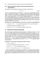
from (7.76) and (7.77), respectively.
Figure
7.4
displays the estimates and true values for
1.5
<
,u
<
5.5
using a single
simulation run of
N
=
lo5
cycles. The simulation was carried out under the service
rate
,G
=
2
and arrival rate
X
=
1.
We see that both
[(p)
and

V'l(p,)
are estimated
accurately over the whole range. Note that for
p
<
2
the confidence interval for
@)
grows rapidly wider. The estimation should not be extended much below
p
=
1.5,
as the importance sampling will break down, resulting in unreliable estimates.
st
=
st-1
+
-
-
st,
t
=
1,2,.
. .
,7
(So
=
0)
,
-4

I
1
2
3
4
5
6
fi
Figure
7.4
as a function
of
p.
Estimated and true values for the expected steady-state waiting time and its derivative
SENSITIVITY
ANALYSIS
OF
DEDS
229
Although (7.76) and (7.77) were derived for the case where the
{Xi}
are iid, much of the
theory can be readily modified to deal with the dependent case. As an example, consider
the case where
XI,
X2,
.
.
.
form an ergodic Markov chain and

R
is of the form
(7.79)
t=l
where
czI
is the cost of going from state
i
to
j
and
R
represents the cost accrued in a cycle of
length
T.
Let
P
=
(pzJ)
be the one-step transition matrix of the Markov chain. Following
reasoning similar to that for (7.67) and defining
Ht
=
CX~-~,X~,
we see that
-
where
P
=
(&)

is another transition matrix, and
is the likelihood ratio. The pdf of
Xt
is given by
t
k=I
The score function can again be obtained by taking the derivative of the logarithm of the
pdf. Since,
&[TI
=
IE,[~~=,
Wt],
the long-run average cost
[(P)
=
IEp[R]/&[T]
can
be estimated via (7.76)
-
and its derivatives by (7.77)
-
simultaneously for various
P
using a single simulation run under
P.
I
1
EXAMPLE
7.13
Markov Chain: Example

4.8
(Continued)
Consider again the two-state Markov chain with transition matrix
P
=
(pij)
and cost
matrix
C
given by
and
respectively, where
p
denotes the vector
(~~,p2)~.
Our goal is to estimate
[(p)
and
Vl(p)
using (7.76) and (7.77) for various
p
from a single simulation run under
6
=
(i,
$)T.
Assume, as
in
Example
4.8,

that starting from state
1,
we obtain
the sample trajectory
(Q,IC~,Q,. . .
,210)
=
(1,2,2,2,1,2,1,1,2,2,l),which
has
four cycles with lengths
T~
=
4,
7-2
=
2,
T~
=
1,
74
=
3
and corresponding
in
the first cycle is given by (7.79). We consider the cases
(1)
p
=
6
=

(i,
i)'
and
(2)
p
=
(i,
f)'.
The transition matrices for the two cases are
transition probabilities
(~12, ~22, ~22, 2321); (~12, ~21); (~11); (~12,~22, ~21).
Thecost
-
P=
(i
!)
and
P=
(i
i)
.
230
SENSITIVITY
ANALYSIS
AND
MONTE
CARL0
OPTIMIZATION
Note that the first case pertains to the nominal Markov chain.
In the first cycle, costs

H11
=
1,
H21
=
3,
H31
=
3,
and
H41
=
2
are incurred.
The likelihood ratios under case
(2)
are
W11
=
=
8/5,
Wz1
=
LVIIF
=
1,
W31
=
W21g
=

and
W41
=
W31a
PZl
=
g,
while in case
(1)
they are all 1.
Next, we derive the score functions (in the first cycle) with respect to
pl
and
pz.
Note
that
PZZ
f4(x4;p)
=p12p;2p21
=
(1
-P1)(1
-P2)2P2.
It follows that in case
(2)
5
-lnfd(xq;p)
=
-
-

dPl
1-Pl
4
-
a
-1
and
a
-2
1
-
In
fd(x4;
p)
=
-
+
-
=
-2
,
8PZ
1
-P2
P2
so
that the score function at time
t
=

4
in the first cycle is given by
s41
=
(-
2,
-2).
Similarly,
S31
=
(-$,
-4),
Szl
=
(-2,
-2), and
S11
=
(-2,O).
The quantities
for the other cycles are derived in the same way, and the results are summarized in
Table 7.3.
Table
7.3
Summary
of
costs, likelihood ratios, and score functions.
By
substituting these values in (7.76) and (7.77), the reader can verify that
@p)

=
1.8,
F(p)
=:
1.81,
%(p)
=
(-0.52, -0.875),and
G(p)
=
(0.22, -1.23).
PROBLEMS
7.1
Consider the unconstrained minimization program
(7.80)
where
X
-
Ber(u)
.
a)
Show that the stochastic counterpart of
W(u)
=
0
can be written (see (7.18)) as
b
UZ
N
h

A
11
71
N
oqu)
=
oqu;
ZJ)
=

c
x,
-
-
=
0
,
t=l
(7.81)
where
XI,.
. .
,
XN
is a random sample from
Ber(w).
PROBLEMS
231
b)
Assume that the sample

{O,l,O,O,l,O,O,l,l,l,O,l,O,l,l,O,l,O,l,l}
was
generated from
Ber(w
=
1/2).
Show that the optimal solution
u*
is estimated as
7.2
Consider the unconstrained minimization program
min!(u)
=
min{lEu[X]
+
bu},
u
E
(0.5,2.0)
,
(7.82)
+
b
=
0
can
11
U
1
where

X
-
Exp(u).
Show that the stochastic counterpart of
Ve(u)
=
-
be written (see
(7.20))
as
e-UXi
(1
-
u
Xi)
N
1
N
oqu;
w)
=
-
1
xi
e-llX'
+b=O,
i=l
(7.83)
where
XI,

.
.
.
,
X,
is a random sample from
Exp(w).
7.3
Prove
(7.25).
7.4
Show that
VkW(x;
u,v)
=
S(k)(~;
x)
W(x;
u,
v)
and hence prove
(7.16).
7.5
Let
Xi
-
N(ui,
cr,"),
i
=

1,
.
. .
,
n
be independent random variables. Suppose we
are interested in sensitivities with respect to
u
=
(~1,.
.
.
,
u,)
only. Show that, for
i
=
1.
. .
.
.
n.
and
[S(')(u;
X)lZ
=
.;2(2,
-
.I)
.

7.6
distributed according to the exponential family
Let the components
X,,
i
=
1,.
.
.
,
n
of a random vector
X
be independent, and
ji(zi;
ui)
=
ci(ui)
ebl(ua)'*(s,)
hi(x:i)
,
where
bi(ui),
ti(zi)
and
hi(zi)
are real-valued functions and
ci(ui)
is normalization con-
stant. The corresponding pdf of

X
is given by
f(x;
u)
=
c(u)
exp
1
bi(ui)ti(zi)
h(x)
,
(a:]
)
where
u
=
CUT,.
. .
,
uf),
c(u)
=
ny=l
ci(ui),
and
h(x)
=
ny=l
hi(zi)
.

a)
Show that Var,(HW)
=
6
lE,[H2]
-
!(u)~,
where
w
is determined by
b)
Show that
bi(wi)
=
2bi(~i)
-
bi(vi),
i
=
I,.
.
.
,n.
EV[H2W2]
=
E"[W2] lE,[H2]
.
7.7
Consider the exponential pdf
f(z;

u)
=
uexp(-uz).
Show that if
H(z)
is a mono-
tonically increasing function, then the expected performancel(u)
=
lE,[H(X)]
is a mono-
tonically decreasing convex function of
u
€
(0,
M).
232
SENSITIVITY
ANALYSIS
AND
MONTE
CARLO
OPTIMIZATION
7.8
function
Let
X
-
N(u.,
02).
Suppose that

cr
is known and fixed.
For
a given
u,
consider the
C(v)
=
IEV[H2W2]
.
a)
Show that if
IE,[H2]
<
cc
for all
u
E
R,
then
L(v)
is convex and continuous on
R.
Show further that if, additionally,
IEu,[H2]
>
0
for any
u,
then

C(v)
has a
unique minimizer,
v*,
over
R.
b)
Show that if
H2(z)
is monotonically increasing on
R,
then
w*
>
u.
7.9
Let
X
-
N(u,
02).
Suppose that
u
is known, and consider the parameterg. Note that
the resulting exponential family is not of canonical form
(A.9).
However, parameterizing
it by
8
=

cr-2
transforms it into canonical form, with
t(5)
=
-(x
-
2~)~/2 and c(6)
=
(2~) -1/261/2.
a)
Show that
provided that
0
<
q
<
26.
b)
Show that, for a given
0,
the function
L(7)
=
IE,[H2W2]
has a unique minimizer,
q*,
on the interval
(0,28),
provided that the expectation,
IE,

[H2],
is finite
for
all
7
E
(0,20)
and does not tend to
0
as
q
approaches
0
or
28. (Notice that this implies that the corresponding optimal value,
cr*
=
~*-l/~,
of the reference parameter,
0,
is also unique.)
c)
Show that if
H2(z)
is strictly convex on
R,
then
q*
<
0.

(Notice that this implies
that
cr*
>
a.)
7.10
Consider the performance
H(X17
x2;"3,"4)
=
min(max(X1,
w),
max(X2,
~4))
,
where
X1
and
X2
havecontinuousdensities
f(z1;
u1)
and
f(z2;
u2),
respectively. If we let
Y1
=
max(
XI,

u3)
and
Y2
=
max( X2,
uq)
and write the performance as
min(Y1
Yz),
then
Y1
and
Y2
would take values
u3
and
u4
with nonzero probability. Hence the random vector
Y
=
(Yl,
Y2)
would not have a density function at point
(u3,11,4),
since its distribution is
a
mixture of continuous and discrete ones. Consequently, the push-out method would fail in
its current form.
To
overcome this difficulty, we carry out a transformation. We first write

and then replace
X
=
(XI,
X2)
by the random vector
X
=
(21,22),
where
and
Prove that the density of the random vector
(21,22)
is differentiable with respect to the
variables
(u3,u4),
provided that both
21
and
22
are greater than
1.
REFERENCES
233
7.1
1
Delta
method.
Let
X

=
(XI,
.
.
.
,
X,)
and
Y
=
(Y1,
. . .
,
Y,)
be random (column)
vectors, with
Y
=
g(X)
for some mapping
g
from
Rn
to
R".
Let
CX
and
Cy
denote the

corresponding covariance matrices. Suppose that
X
is
close to its mean
p.
A first-order
Taylor expansion of
g
around
p
gives
y
=
P(P)
+
J,(g)(X
-
where
J,(g)
is the matrix of Jacobi of
g
(the matrix whose (z,j)-th entry is the partial
derivative
agi/azj)
evaluated at
p.
Show that, as a consequence,
This is called the
delta method
in statistics.

Further Reading
The SF method in the simulation context appears to have been discovered and rediscovered
independently, starting in the late 1960s. The earlier work on SF appeared in Aleksandrov,
Sysoyev, and Shemeneva [l] in 1968 and Rubinstein [14] in 1969. Motivated by the
pioneering paper of
Ho,
Eyler, and Chien [6] on
infinitesimal perturbation analysis
(IPA)
in 1979, the SF method was rediscovered at the end of the 1980s by Glynn [4] in 1990 and
independently in
1989
by Reiman and Weiss
[
121, who called it the
likelihoodratio method.
Since then, both the IPA and SF methods have evolved over the past decade or
so
and have
now reached maturity; see Glasserman
[3],
Pflug [ll], Rubinstein and Shapiro [18], and
Spa11 [20].
To
the best of our knowledge, the stochastic counterpart method in the simulation context
was first suggested by Rubinstein in his PhD thesis [14]. It was applied there to estimate
the optimal parameters in a complex simulation-based optimization model. It was shown
numerically that the
off-line
stochastic counterpart method produces better estimates than the

standard
on-line
stochastic approximation. For some later work on the stochastic counterpart
method and stochastic approximation, see
[
151. Alexander Shapiro should be credited
for developing theoretical foundations for stochastic programs and, in particular, for the
stochastic counterpart method. For relevant references, see Shapiro's elegant paper
[
191
and also
[
17, 181. As mentioned, Geyer and Thompson
[2]
independently discovered the
stochastic counterpart method in the early 199Os, and used it to make statistical inference
in a particular unconstrained setting.
REFERENCES
I.
V.
M
Aleksandrov,
V.
I.
Sysoyev, and
V.
V.
Shemeneva. Stochastic optimization.
Engineering
2.

C.
J.
Geyer and
E.
A.
Thompson. Annealing Markov chain Monte-Carlo with applications to
3.
P.
Glasseman.
Gradient Estimation via Perturbation Analysis.
Kluwer, Norwell, Mass., 1991.
4.
P.
W.
Glynn. Likelihood ratio gradient estimation for stochastic systems.
Communications
of
5.
D.
Gross
and C. M. Hams.
Fundamentals
of
Queueing
Theory.
John Wiley
&
Sons, New York,
Cybernetics,
5:

11-16, 1968.
ancestral inference.
Journal
of
ihe
American Statisiical Association,
90:909-920, 1995.
the
ACM,
33(10):75-84, 1990.
2nd edition, 1985.
234
SENSITIVITY ANALYSIS AND MONTE CARL0 OPTIMIZATION
6. Y. C.
Ho,
M.
A.
Eyler, and T.
T.
Chien.
A
gradient technique for general buffer storage design in
a serial production line. International Journal
on
Production Research, 17(6):557-580, 1979.
7.
J.
Kiefer and
J.
Wolfowitz. Stochastic estimation of the maximum

of
regression function. Annals
8.
A.
I.
Kleywegt and
A.
Shapiro. Stochastic optimization. In
G.
Salvendy, editor, Handbook
of
9.
A.
J.
Kleywegt,
A.
Shapiro, and
T.
Homern de Mello. The sample average approximation method
10. H.
J.
Kushner and
D.
S.
Clark. Stochastic Approximation Methods for Constrained and Uncon-
11.
G.
Ch.
Pflug.
Optimization

of
Stochastic Models. Kluwer, Boston, 1996.
12. M.
I.
Reiman and
A.
Weiss. Sensitivity analysis for simulations via likelihood ratios. Operations
13.
H.
Robbins and
S.
Monro. Stochastic approximation methods. Annals
ofMathematicalStatistics,
14.
R.
Y.
Rubinstein. Some Problems
in
Monte Carlo Optimization.
PhD
thesis, University of Riga,
15. R.
Y.
Rubinstein. Monte Carlo Optimization Sirnulation and Sensitivity
of
Queueing
Network.
16.
R.
Y. Rubinstein and

B.
Melamed. Modern Simulation and Modeling. John Wiley
&
Sons, New
17. R. Y. Rubinstein and
A.
Shapiro. Optimization
of
static simulation models by the score function
18. R.
Y.
Rubinstein and
A.
Shapiro. Discrete Event Systems; Sensitivity Analysis and Stochastic
19.
A.
Shapiro.
Simulation based optimization: convergence analysis and statistical inference.
20. J.
C.
Spall. Introduction to Stochastic Search and Optimization; Estimation, Simulation, and
of
Mathematical Statistics, 23:462-466, 1952.
Industrial Engineering, pages 2625-2650, New York, 2001. John Wiley
&
Sons.
for stochastic discrete optimization. SlAM Journal
on
Optimization, 12:479-502, 2001.
strained Systems. Springer-Verlag, New York, 1978.

Research, 37(5):83&844, 1989.
22:400407, 195
1.
Latvia, 1969. (In Russian).
John Wiley
&
Sons, New York, 1986.
York, 1998.
method. Mathematics and Computers in Simulation, 32:373-392, 1990.
Optimization via the Score Function Method. John Wiley
&
Sons, New York, 1993.
Stochastic Models, 12:425454, 1996.
Control. John Wiley
&
Sons, New York, 2003.
CHAPTER
8
THE CROSS-ENTROPY METHOD
8.1
INTRODUCTION
The
cross-entropy
(CE) method
[3
11
is
a relatively new Monte Carlo technique for both
estimation and optimization. In the estimation setting, the CE method provides an adaptive
way to find the optimal importance sampling distribution for quite general problems.

By
formulating an optimization problem as an estimation problem, the CE method becomes a
general and powerful stochastic search algorithm. The method is based on a simple iterative
procedure where each iteration contains two phases: (a) generate a random data sample
(trajectories, vectors, etc.) according to a specified mechanism; (b) update the parameters
of the random mechanism on the basis of the data in order to produce a better sample in the
next iteration.
The
CE
method has its origins in an adaptive algorithm for rare-event estimation based
on
varianceminimization
(VM)
[26].
This procedure was soon modified
[27]
to an adaptive
algorithm for both rare-event estimation and combinatorial optimization, where the original
VM
program was replaced by a similar CE minimization program. In this chapter we present
a general introduction to the
CE
method. For a comprehensive treatment we refer to
[3
11.
The rest of this chapter is organized as follows. Section
8.2
presents a general CE
algorithm for the estimation of rare-event probabilities, while Section
8.3

introduces a slight
modification of this algorithm for solving combinatorial optimization problems. We discuss
applications of the
CE
method
to
several such problems, such as the max-cut problem and
the
TSP,
and provide supportive numerical results on the performance of the algorithm.
Simulation and the Monte
Carlo
Method Second Edition.
By R.Y. Rubinstein
and
D.
P.
Kroese
Copyright
@
2007
John
Wiley
&
Sons,
Inc.
235
236
THE
CROSS-ENTROPY

METHOD
Finally, in Sections 8.7 and 8.8 we show how the CE method can deal with continuous and
noisy optimization problems, respectively.
8.2 ESTIMATION
OF
RARE-EVENT PROBABILITIES
In this section we apply the
CE
method in the context of efficient estimation of small
probabilities. Consider, in particular, the estimation of
e
=
PU(S(X)
2
7)
=
Eu
[qs(X)>y}l
(8.1)
for some fixed level
y.
Here
S(X)
is
the sample performance,
X
is a random vector with
pdf
j(.;
u)

belonging to some parametric family
{f(.;v),v
E
"Y},
and
{S(X)
y}
is
assumed to be a rare event. We can estimate
l
using the likelihood ratio estimator (see also
.N
(5.59))
where
XI,.

,XN
is a random sample from
f(x;v)
and
w(xk;u,v)
=
f(Xk; u)/f(Xk; v)
is the likelihood ratio.
EXAMPLE
8.1
Stochastic Shortest Path
Let
us
return to Example 5.14 (see also Example 5.1). where the objective is to

efficiently estimate the probability
e
that the shortest path from node
A
to node
B
in
the network of Figure 8.1 has a length of at least
y.
The random lengths
XI
.
.
.
,
X5
of the links are assumed to be independent and exponentially distributed with means
211,
. . .
,
u,5,
respectively.
Figure
8.1
Shortest path
from
A
to
B.
Defining

X
=
(XI,.
.
.
,
Xs),
u
=
(2~1,.
.
.
us)
and
S(X)
=
min{X1+
X4,
XI
+
X3
+
X5,
X2
+
X5, X2
+
X3
+
X4},

the problem is cast in the framework of (8.1).
As
explained in Example 5.14, we can
estimate (8.1) via (8.2) by drawing
XI,
.
. .
,
X5
independently from exponential dis-
tributions that are possibly
dferent
from the original ones. That is,
Xi
N
Exp(vzrl)
instead of
Xi
N
Exp(u,'),
i
=
1,.
. .
,5.
The corresponding likelihood ratio was
given in (5.73).
ESTIMATION
OF
FARE-EVENT PROBABILITIES

237
The challenging problem is how to select a vector
v
=
(v1,
.
.
.
,w5)
that gives the
most accurate estimate of
e
for a given simulation effort. In the toy Example
5.14,
this was achieved by first choosing the trial vector
w
equal to
u
and then applying the
CE updating formula (5.69), possibly iterating the latter. This approach was possible
because the event
{
S(x)
2
y}
was
not rare.
However, for the current problem (5.69)
cannot be applied directly, since for rare events it returns, with high probability,
the indeterminate expression

1.
To
overcome this difficulty, we will use a different
approach to selecting a
good
v
by adopting a
two-stage
procedure where
both the
level
y
and the reference parameters
v
are updated.
One of the strengths of the CE
method for rare-event simulation
is
that it provides a fast way to estimate accurately
the optimal parameter vector
v*.
Returning to the general situation, we have seen in Section
5.6
that for estimation prob-
lems of the form (8.1) the ideal (zero variance) importance sampling density is given by
which is the conditional pdf of
X
given S(X)
2
y.

The idea behind the CE method is
to get as close as possible to the optimal importance sampling distribution by using the
Kullback-Leibler CE distance as a measure of closeness. Using a parametric class of
densities
{f(x;
v),v
E
Y},
this means (see (5.61)) that the optimal reference parameter
v*
is given by
V*
=
argmaxEu[Z{s(x)aY}
lnf(X;v)l
.
(8.3)
VEY
We can, in principle, estimate
V*
as
with XI,
.
. .
,
XN
N
f(.;
u)
-

that is, using the stochastic counterpart of (8.3). However,
as mentioned in Example 8.1, this is void of meaning if
{
S(X)
2
y}
is a rare event under
f(.;
u),
since then most likely all indicators in the sum above will be zero.
To
circumvent this problem we shall use a multilevel approach where we generate a
sequence of reference parameters
{
vt,
t
2
0)
and a sequence
of
levels
{yt,
t
3
1)
while
iterating in both
yt
and
vt.

Our ultimate goal is to have
vt
close to
v*
after some number
of iterations and to use
vt
in the importance sampling density
f(.;
vt) to estimate
t.
We start with
vo
=
u.
Let
e
be a not
too
small number, say
lo-'
<
Q
<
lo-'.
In the
first iteration, we choose
v1
to
be the optimal parameter for estimating PU(S(X)

2
TI),
where
y1
is
the
(1
-
Q)-quantile of S(X). That is,
y1
is the largest real number for which
Thus, if we simulate under
u,
then level y1
is
reached with a reasonably high probability of
around
e.
This enables
us
to estimate both
y1
and
v1
via Monte Carlo simulation. Namely,
we can estimate y1 from a random sample XI,
.
.
.
,

XN
from
f(.;
u)
as follows. Calculate
the performances S(X,) for all
i,
and order them from smallest to largest:
S(l)
<
.
.
.
<
S(N).
Then
y1
is estimated via the sample
(1
-
Q)-quantile
=
S(r(l-e)~l),
where
[a1
denotes the smallest integer larger than
or
equal to
a
(the so-called

ceiling
of
a).
The
reference parametervl can be estimated via (8.4), replacing
y
with the estimate of
y1.
Note
that we can use here the
same
sample for estimating both
v1
and
71.
This means that
v1
is
238
THE
CROSS-ENTROPY
METHOD
estimated on the basis of the
[e
N1
best samples, that is, the samples
Xi
for which
S(Xi)
is greater than or equal to

TI.
These form the
elite samples
in the first iteration; let
Ne
denote the number of elite samples.
In the subsequent iterations we repeat these steps. Thus, we have the following two
updating phases, starting from
vo
=
GO
=
u:
1.
Adaptive updating of
-yt.
For
a fixed
vtPl,
let
yt
be the
(1
-
Q)-quantile of
S(X)
under
~~-1.
To
estimate

-yt,
draw a random sample
XI,
.
.
.
,
XN
from
f(.;
Vt-l)
and
evaluate the sample
(1
-
Q)-quantile
Tt.
2.
Adaptive updating of
vt.
For fixed
yt
and
vt
-
1,
derive
vt
as
vt

=
argmax%-,
[I~s(x)~~~~W(X;U,V~-~)~~~(X;~)]
.
(8.5)
The stochastic counterpart of
(8.5)
is as follows: for fixed
Tt
and
Gt-l,
derive
Gt
as
the solution
VEY
where
&,
is the
set
of
elite samples
in the t-th iteration, that is, the samples
Xk
for
which
S(Xk)
2
Tt.
The procedure terminates when at some iteration

T
a level
TT
is
reached that is at least
y
and thus the original value of
y
can be used without getting too few samples. We then
reset
TT
to
y,
reset the corresponding elite set, and deliver the final reference parameter
G*,
again using
(8.6).
This
C*
is then used in
(8.2)
to estimate
C.
The resulting
CE
algorithm for rare-event probability estimation can thus be written as
follows.
Algorithm 8.2.1 (Main
CE
Algorithm for Rare-Event Estimation)

1.
Define
GO
=
u.
Let
Ne
=
[(l
-
e)N].
Set
t
=
1
(iteration counter).
2.
Generate a random sample
XI,
. . .
,
XN
according to thepdf
f(.;
Gt-l).
Calculate
the perjiormances
S(X,)
for all
i,

and order them from smallest to largest,
S(1)
<
.
.
.
<
S(N).
Let
Tt
be the sample
(1
-
e)-quantile ofperjiormances:
yt
=
S(Ne).
rf
qt
>
y,
reset
Ft
to
y.
3.
Use the
same
sample
X1,

. .
.
,
XN
to solve the stochasticprogram
(8.6).
4.
If
Tl
<
y,
set
t
=
t
+
1
and reiterate from Step
2.
Otherwise, proceed with Step
5.
5.
Let
T
be the
final
iteration counter: Generate a sample
XI,
.
.

.
,
XN,
according to
thepdf
f(.;
VT)
andestimate
C
via
(8.2),
Remark 8.2.1
In typical applications the sample size
N
in Steps 24can be chosen smaller
than the final sample size
N1
in Step
5.
Note that Algorithm
8.2.1
breaks down the complex problem of estimating the very small
probability
C
into a sequence of simple problems, generating a sequence of pairs
{
(Tt,
Vt)},
ESTIMATION
OF

RARE-EVENT
PROBABILITIES
239
depending on
e,
which is called the
rarityparameter.
Convergence of Algorithm
8.2.1
is
discussed in
[3
11. Other convergence proofs for the CE method may be found in
[21]
and
[61.
Remark 8.2.2 (Maximum Likelihood Estimator)
Optimization problems of the form
(8.6)
appear frequently in statistics. In particular, if the
W
term is omitted
-
which
will turn out to be important in CE optimization
-
one can also write
(8.6)
as
A

vt
=
argmax
I-J
f(~k;v)
,
XkEEt
where the product is the joint density of the elite samples. Consequently,
?t
is chosen
such that the joint density of the elite samples is maximized. Viewed as a function of the
parameter
v,
rather than of the data
{&t},
this joint density is called the
likelihood.
In other
words,
Gt
is the
maximum likelihood estimator
(it maximizes the likelihood) of
v
based on
the elite samples. When the
W
term is present, the form of the updating formula remains
similar. Recall from Section
5.6

that for exponential families the updating rules for
?t
can
be obtained analytically; see also Section A.3
of
the Appendix.
To
gain a better understanding of the CE algorithm, we also present its
deterministic
version.
Algorithm 8.2.2 (Deterministic Version
of
the
CE
Algorithm)
I.
Dejine
vg
=
u.
Set
t
=
1
2.
Calculate
-yt
as
-yt
=

max
{s
:
Pvt-,(S(X)
>
3)
>
e}
.
(8.7)
If-yt
>
7,
reset
-yt
to
y.
3.
Calculate
vt
(see
(8.5))
as
4.
rfrt
=
y
stop;
otherwise, set
t

=
t
+
1
and repeatfrom Step
2.
Note that, when compared with Algorithm
8.2.1,
Step
5
is redundant in Algorithm 8.2.2.
number of toy examples.
To
provide further insight into Algorithm 8.2.1, we shall follow it step by step in a
EXAMPLE
8.2
Exponential Distribution
Let
us
revisit Examples
5.8,5.10,
and 5.12, where the goal was to estimate, via Monte
Carlo simulation, the probability
e
=
P,(X
2
y),
with
X

-
Exp(u-').
Suppose
that
y
is large in comparison with
u,
so
that
C
=
e-YIu
is
a rare-event probability.
The updating formula for
Zt
in
(8.6)
follows from the optimization of
240
THE
CROSS-ENTROPY
METHOD
where
wk
=
e-Xk(u-l-y-')v/u.
To
find the maximum of the right-hand side, we
take derivatives and equate the result to

0:
Solving this for
v
yields
Gt.
Thus,
In other words,
Gt
is simply the sample mean of the elite samples weighted by the
likelihood ratios. Note that without the weights
{
wk}
we would simply have the
maximum likelihood estimator of
v
for the
Exp(v-')
distribution based on the elite
samples in accordance with Remark 8.2.2. Note also that the updating formula
(8.9)
follows directly from
(5.69).
Similarly, the
deterministic
updating formula
(8.8)
gives
where
yt
is

the (1
-
p)-quantileof the
Exp(~;-'~)
distribution. Thus,
-yt
=
-1.~t-1
In
p.
Assume for concreteness that
u
=
1
and
y
=
32, which corresponds to
e
=
1.2710-14. Table
8.1
presents the evolution of
Tt
and
Gt
for p
=
0.05
using sample

size
N
=
1000. Note that iteration
t
=
0
corresponds to the original exponential
pdf with expectation
u
=
1,
while iterations
t
=
1,2,3 correspond to exponential
pdfs with expectations
Gt,
t
=
1,2,3, respectively. Figure
8.2
illustrates the iterative
procedure. We see that Algorithm 8.2.1 requires three iterations to reach the final
level
73
=
32. In the third iteration the lowest value of the elite samples,
S(N'),
was

in fact greater than 32,
so
that in the final Step 2 of the algorithm we take
y3
=
y
=
32
instead. The corresponding reference parameter
G3
was found to be 32.82. Note that
both parameters
Tt
and
Gt
increase gradually, each time "blowing up" the tail of the
exponential pdf.
The final step of Algorithm 8.2.1 now invokes the likelihood ratio estimator (8.2)
to estimate
e,
using a sample size
N1
that is typically larger than
N.
Table
8.1
The evolution
of
Tt
and

Gt
for
Q
=
0.05
with
y
=
32,
using
N
=
1000
samples.
t
7t
Gt
0-
1
1
2.91 3.86
2 11.47 12.46
3
32 32.82
ESTIMATION
OF
RARE-EVENT
PROBABILITIES
241
Figure

8.2
A three-level realization
of
Algorithm
8.2.1.
Each shaded region has area
Q.
EXAMPLE
8.3
Degeneracy
When
y
is the maximum of
S(x),
no “overshooting” of
y
in Algorithm
8.2.1
occurs
and therefore
yt
does not need to be reset. In such cases the sampling pdf may
degenerate
toward the
atomic
pdf that has all its mass concentrated at the points
x
where
S(x)
is maximal. As an example, suppose we use a

Beta(v,
l),
v
2
1
family
of importance sampling distributions, with nominal parameter
u
=
1
(corresponding
to the uniform distribution), and take
S(X)
=
X
and
y
=
1.
We find the updating
formula for
v
from the optimization of
with
wk
=
l/(vX;-’).
Hence,
Table
8.2

and Figure
8.3
show the evolution of parameters in the
CE
algorithm using
Q
=
0.8
and
N
=
1000.
We see that
Tt
rapidly increases to
y
and that the sampling
pdf degenerates to the atomic density with mass at
1.
Table
8.2
using
N
=
1000
samples.
The evolution
of
Tt
and

Gt
for
the
Beta(v,
1)
example, with
Q
=
0.8
and
7
=
1,
t
Tt
I’t
t
?t
Ut
0-
1
5
0.896 31.2
1
0.207 1.7
6
0.949 74.3
2
0.360
3.1

7
0.979 168.4
3
0.596
6.4
8
0.990
396.5
4
0.784 14.5
9
0.996 907.7
242
I
I
30
h
6
I
K
20
I
I
I
I
I
v
\
10
0

1
0
0.2
0.4
0.6
0.8
m
Figure
8.3
Degeneracy
of
the sampling distribution.
EXAMPLE
8.4
Coin
Flipping
Consider the experiment where we flip
n
fair coins. We can describe this experiment
via
n
independent Bernoulli random variables,
XI,
.
.
.
,
X,,
each with success pa-
rameter 1/2. We write

X
=
(XI,.
.
.
,Xn)
-
Ber(u),
where
u
=
(1/2,.
. .
,
l/2)
is the vector of success probabilities. Note that the range
of
X
(the set
of
possible
values it can take) contains 2" elements. Suppose we are interested in estimating
e
=
Pu(S(X)
2
y),
with
S(X)
=

EL=,
xk.
We want to employ importance sam-
pling using
X
-
Ber(p)
for a possibly different parameter vector
p
=
(PI,.
.
.
,
p,).
Consider two cases: (a)
y
=
(n
+
1)/2 (with
n
odd) and (b)
y
=
n.
It is readily
seen that for cases (a) and (b) the optimal importance sampling parameter vector is
p*
=

(1/2,.
. .
,1/2) and
p*
=
(1,.
.
.
,
l), respectively. The corresponding prob-
abilities are
e
=
4
and
C
=
&,
respectively. Note that in the first case
C
is not a
rare-event probability, but
it
is
so
for the second case (provided that
n
is large). Note
also that in the second case
Ber(p*)

corresponds to a
degenerated
distribution that
places all probability mass at the point (1,1,.
.
.
,
1).
Since
{
Ber(p)}
forms an exponential family that is parameterized by the mean, it
immediately follows from
(5.69)
that the updating formula for
p
in Algorithm
8.2.1
at the t-th iteration coincides with
(8.9)
and is given by
,
i
=
1,
,
n,
Exkc&,
wk
Xki

Pt,;
=
CXk&t
wk
(8.10)
where
Xki
is the i-th component of the k-th sample vector
xk
-
Ber(&-
I),
and
wk
is the corresponding likelihood ratio:
n
i=l
with
qi
=
po,i/&l,i and
~i
=
(1
-
po,,)/(l
-
Ft-l,i),
i
=

1,.
.
.
,
n.
Thus, the i-th
probability is updated as a weighted average of the number of
1
s
in the i-th position
over all vectors in the elite sample.
As
we shall see below, this simple coin flipping example will shed light on how
rare-events estimation is connected with combinatorial optimization.
ESTIMATION
OF
RARE-EVENT PROBABILITIES
243
Remark
8.2.3
It is important to note that if we employ the deterministic CE algorithm
8.2.2 to any rare-event-type problem where the underlying distributions have finite supports
withoutfiing
y
in
advance,
it will iterate until it reaches some
y,
denoted as
y,

(not
necessarily the true optimal
y*),
and then stop. The corresponding importance sampling
pdf
f(x;
v,)
will be
degenerated.
For the above coin flipping example we will typically
have in case (b) that
y*
=
y*
=
n.
The main Algorithm 8.2.1 behaves similarly, but in a
stochastic rather than a deterministic sense. More precisely, for pdfs with finite supports and
y
not fixed in advance, it will generate a tuple
(TT,
GT)
with
f(x;
GT)
corresponding again
typically to a degenerate pdf. This property of Algorithms 8.2.2 and 8.2.1 will be of crucial
importance when dealing with combinatorial optimization problems in the next section. As
mentioned, a combinatorial optimization problem can be viewed as a rare-event estimation
problem in the sense that its optimal importance sampling pdf

f(x;
v*)
is a degenerated
one and coincides with the one generated by the deterministic rare-event Algorithm 8.2.2,
provided that it keeps iterating in
y
without fixing it in advance.
In the next example, we illustrate the behavior of Algorithm 8.2.1 when applied to a
typical static simulation problem of estimating
l
=
P(S(X)
2
7).
Note that the likelihood
ratio estimator Fof
e
in (8.2)
is
of the form
i=
N-'
C;=,
Zk.
We measure the efficiency
of the estimator by its relative error (RE), which (recall
(4.10))
is defined as
and which is estimated by
S/(?fi),

with
N
k=l
being the sample variance of the
{
Zi}.
Assuming asymptotic normality of the estimator, the
confidence intervals now follow in a standard way. For example, a
95%
relative confidence
interval for
l
is given by
F3z
1.96
ZRE
.
EXAMPLE
8.5
Stochastic Shortest Path: Example
8.1
(Continued)
Consider again the stochastic shortest path graph of Figure
8.1.
Let
us
take the same
nominal parameter vector
u
as in Example

5.14,
that is,
u
=
(1,
1,0.3,0.2,0.1),
and
estimate the probability
e
that the minimum path length is greater than
y
=
6.
Note
that in Example
5.14
y
=
1.5 is used, which gives rise to an event that is not rare.
Crude Monte Carlo (CMC), with
10'
samples
-
a very large simulation effort
-
gave an estimate 8.01
.
To
apply Algorithm 8.2.1 to this problem, we need to establish the updating rule
for the reference parameter

v
=
(ul,
. . .
,
w5).
Since the components
X1
,
.
. .
,
X5
are
independent and form an exponential family parameterized by the mean, this updating
formula follows immediately from
(5.69),
that is,
with an estimated relative error of 0.035.
with
W(X;
u,
v)
given in
(5.73).
244
THE CROSS-ENTROPY METHOD
A
Yt
1.1656

2.1545
3.1116
4.6290
6.0000
We take
in
all our experiments
with
Algorithm 8.2.1 the rarity parameter
e
=
0.1,
the sample size for Steps 24 of the algorithm
N
=
lo3,
and for the final sample size
N1
=
lo5. Table 8.3 displays the results of Steps
14
of the CE algorithm. We see
that after five iterations level
y
=
6 is reached.
"1
1
.OOOO
1

.OOOO
0.3000 0.2000 0.1000
1.9805 2.0078 0.3256 0.2487 0.1249
2.8575 3.0006 0.2554 0.2122 0.0908
3.7813 4.0858 0.3017 0.1963 0.0764
5.2803 5.6542 0.2510 0.1951
0.0588
6.7950 6.7094 0.2882 0.1512 0.1360
t
0
1
2
3
4
5
-
Using the
0.2882,
with an
-
estimated optimal parameter vector of
65
=
(6.7950,6.7094,
0.1512,0.1360), Step
5
of the CE algorithm gave an estimate of 7.85.
estimated relative error of 0.035
-
the same as for the CMC method

with
lo8
samples. However, whereas the CMC method required more than an hour of
computation time, the CE algorithm was finished in only one second, using a Matlab
implementation on a 1500 MHz computer. We see that with a minimal amount of
work, we have achieved a dramatic reduction of the simulation effort.
Table 8.4 presents the performance of Algorithm 8.2.1 for the above stochastic
shortest path model, where instead of the exponential random variables we used
Weib(ai,
Xi)
random variables,
with
ai
=
0.2
and
Xi
=
u;',
i
=
1,.
. .
,5, where
the
{u,}
are the same as before, that is,
u
=
(1,1,0.3,0.2,0.1).

Table
8.4
and
a
=
0.2.
The
estimated
probability
is
f!
=
3.30.
The
evolution
of
Gt
for
estimagng the
optimal
parameter
v*
with
the
TLR
method
RE
=
0.03.
3.633 2.0367

2.1279 0.9389
1.3834 1.4624
100.0
3.2690 3.3981
1.1454 1.3674 1.2939
805.3 4.8085
4.7221 0.9660
1.1143 0.9244
4 5720 6.6789
6.7252
0.6979 0.9749 1.0118
5
10000
7.5876
7.8139 1.0720
1.3152 1.2252
The Weibull distribution
with
shape parameter
a
less than
1
is an example of a
heavy-fuileddistribution.
We use the TLR method (see Section 5.8) to estimate
e
for
y
=
~O,OOO.

Specifically, we first write (see (5.98))
xk
=
uk~:'~,
with
Zk
-
Exp(
l),
and then use importance sampling on the
{
Zk},
changing the mean of
21,
from
1
to
vk,
k
=
1,.
.
. ,5. The corresponding updating formula is again of the form (8.1
I),
namely,
-
A
cf='=,
I{g(z,)ayt)W(Zk;
1,

6L-1)
zki
c,"=,
1{Sp,)2Tt)W(Zk;
l>Gt-l)
Vt,i
=
-
,
i
=
1,
,
5,