SIMULATION AND THE MONTE CARLO METHOD Episode 11 pps

280
COUNTING
VIA
MONTE
CARL0
Some other #P-complete problems include counting the number of perfect matches in a
bipartite graph, determining the permanent of a matrix, counting the number of fixed-size
cliques in a graph, and counting the number of forests in a graph.
It is interesting to note [23,30] that in many cases the counting problem is hard to solve,
while the associated decision or optimization problem is easy; in other words,
decision is
easy, counting
is
hard.
For example, finding the shortest path between two fixed vertices in
a graph is easy, while finding the total number of paths between the two vertices is difficult.
In this chapter we show how #P-complete counting problems can be viewed as particular
instances
of estimation
problems, and as such can be solved efficiently using Monte Carlo
techniques, such as importance sampling and MCMC. We also show that when using the
standard CE method to estimate adaptively the optimal importance sampling density, one
can encounter degeneracy in the likelihood ratio, which leads to highly variable estimates for
large-dimensional problems. We solve this problem by introducing a particular modification
of the classic
MinxEnt
method
[17],
called the
parametric MinxEnt
(PME) method. We

show that PME is able
to
overcome the
curse
of
the dimensionality
(degeneracy) of the
likelihood ratio by decomposing it into low-dimensional parts. Much of the theory is
illustrated via the satisfiability counting problem in the conjunctive normal form (CNF),
which plays a central role in NP completeness. We also present here a different approach,
which is based
on
sequential sampling. The idea is to break a difficult counting problem into
a combination of easier ones. In particular, for the SAT problem in the disjunctive normal
form (DNF), we design an importance sampling algorithm and show that it possesses nice
complexity properties.
Although #P-complete problems, and in particular SAT, are
of
both theoretical and
practical importance and have been well studied for at least a quarter of a century, we are
not aware of any generic deterministic or randomized method
forfast
counting for such
problems. We are not even aware of any benchmark problems to which our method can be
compared. One goal of this chapter is therefore to motivate more research and applications
on #P-complete problems,
as
the original CE method did in the fields of Monte Carlo
simulation and simulation-based optimization in recent years.
The rest of this chapter is organized as follows. Section 9.2 introduces the SAT counting

problem. In Section 9.3 we show how a counting problem can be reduced to a rare-event
estimation one.
In
Section
9.4
we consider a sequential sampling plan, where a difficult
counting problem
I
X*
I
can be presented as a combination of associated easy ones. Based
on
the above sequential sampling we design an efficient importance sampling algorithm.
We show that for the SAT problem in the DNF form the proposed algorithm possesses
nice complexity properties. Section 9.5 deals with SAT counting in the CNF form, using
the rare-event approach developed in Section 9.3. In particular, we design an algorithm,
called the PME algorithm, which is based on a combination of importance sampling and
the classic MinxEnt method.
In
Section
9.6
we show that the PME method can be applied
to combinatorial optimization problems as well and can be viewed as an alternative to the
standard CE method. The efficiency of the PME method is demonstrated numerically in
Section 9.7.
In
particular, we show that PME works at least as well as the standard CE
for combinatorial optimization problems and substantially outperforms the latter for SAT
counting problems.
9.2 SATlSFlABlLlTY PROBLEM

The Boolean satisfiability (SAT) problem plays a central role in combinatorial optimization
and, in particular, in NP completeness. Any NP-complete problem, such as the max-cut
SATISFIABILITY PROBLEM
281
problem, the
graph-coloring problem,
and the TSP, can be translated
in polynomial time
into
a SAT problem. The SAT problem plays a central role in solving large-scale computational
problems, such as planning and scheduling, integrated circuit design, computer architecture
design, computer graphics, image processing, and finding the folding state
of
a protein.
There are different formulations for the SAT problem, but the most common one, which
we discuss next, consists
of
two components
[
121:
0
A set
of
n
Boolean variables
(21,
.
. . ,
zn},
representing statements that can either be

TRUE
(=1)
or FALSE
(=O).
The negation (the logical NOT)
of
a variable
2
is denoted
by
5.
For example,
=
FALSE. A variable or its negation is called a
literal.
0
A set
of
m
distinct
clauses
{
C1,
Cz,
. . .
,
Cm}
of
the form
Ci

=
zil
V
Ziz
V
. . .
V
zik
where the
z’s
are literals and the
V
denotes the logical
OR
operator. For example,
OVl=l.
The binary vector
x
=
(21,
. . .
,
2,)
is called a
truth assignment,
or simply an
assign-
ment.
Thus,
zi

=
1
assigns truth to
xi
and
xi
=
0
assigns truth to
Zi
for each
i
=
1, .
.
.
,
n.
The simplest SAT problem can now be formulated as:
find a truth assignment
x
such that
all
clauses are
true.
Denoting the logical
AND
operator by
A,
we can represent the above SAT problem via a

single formula as
F1
=
C1
AC2
A
where the
{
Ck}
consist
of
literals connected with only
V
operators. The SAT formula is
said to be in
conjunctive normal
form
(CNF).
An alternative SAT formulation concerns
formulas
of
the type
Fz
=
C1
V
C2
V

V

C,
,
where the clauses are of the form
Ci
=
zil
A
ziz
A
.
.
.
A
zik.
Such a SAT problem is then
said to be in
disjunctive
normal
form
(DNF). In this case, a truth assignment
x
is sought
that satisfies
at least one
of the clauses, which is usually a much simpler problem.
EXAMPLE9.1
As an illustration of the SAT problem and the corresponding SAT counting problem,
consider the following toy example of coloring the nodes
of
the graph in Figure

9.1.
Is
it possible to color the nodes either black or white in such a way that no two adjacent
nodes have the same color?
If
so,
how many such colorings are there?
3
Figure
9.1
color?
Can the graph be colored with two colors
so
that
no
two adjacent nodes have the same
282
COUNTING
VIA
MONTE
CARLO
We can translate this graph coloring problem into a SAT problem in the following
way: Let
x3
be the Boolean variable representing the statement “the j-th node is
colored black”. Obviously,
x3
is either TRUE
or
FALSE, and we wish to assign truth

to either
x3
or
T3,
for each
j
=
1,
. . .
,5.
The restriction that adjacent nodes cannot
have the same color can be translated into a number of clauses that must all hold.
For
example, “node 1 and node 3 cannot both be black” can be translated as clause
C1
=
:1
V
T3.
Similarly, the statement “at least one of node
1
and node
2
must
be
black” is translated as
C2
=
51
V

23.
The same holds for all other pairs of adjacent
nodes. The clauses can now be conveniently summarized as in Table 9.1. Here, in
the left-hand table, for each clause
C,
a
1
in column
j
means that the clause contains
x3,
a
-
1
means that the clause contains the negation
Tj;
and a
0
means that the clause
does not contain either of them. Let us call the corresponding matrix
A
=
(atj)
the
clause
matrix.
For
example,
a75
=

-
1
and
a42
=
0.
An alternative representation
of the clause matrix is to list for each clause only the indices of all Boolean variables
present in that clause. In addition, each index that corresponds to a negation of
a
variable is preceded by a minus sign; see Table 9.1.
Table
9.1
A
SAT
table
and
an alternative representation
of
the clause matrix.
12345
01010
-1
0
-1
0
0
10100
-1
0

0
0
-1
10001
0
-1 -1
0
0
01100
0
-1
0 0
-1
01001
0
0
-1
-1
0
00110
0
0 0
-1
-1
00011
-1
-3
13
-1
-5

15
-2
-3
23
-2
-5
25
-3
-4
34
-4
-5
45
Now let
x
=
(zl,
.
.
.
55)
be a truth assignment. The question is whether there
exists an
x
such that all clauses
{
Ck}
are satisfied.
To
see if a single clause

ck
is
satisfied, one must compare the truth assignment for each variable in that clause with
the values
l,-l,
and
0
in the clause matrix
A,
which indicates if the literal corresponds
to the variable, its negation,
or
that neither appears in the clause. If, for example,
z3
=
0
and
at3
=
-1,
then the literal
Z3
is TRUE. The entire clause is TRUE if it
contains at least one true literal. Define the clause value
C,(x)
=
1
if clause
C,
is

TRUE with truth assignment
x
and
C,(x)
=
0
if it is FALSE. Then it is easy to see that
G(x)
=
max(0,
(2
z3
-
1)
arj
1
,
(9.1)
3
assuming that at least one
a,3
is nonzero for clause
C,
(otherwise, the clause can be
deleted).
For
example, for truth assignment
(0,1,0,1,0)
the corresponding clause
values are given in the rightmost column of the lefthand table in Table

9.1.
We
see
that
SATISFIABILITY
PROBLEM
283
the second and fourth clauses are violated. However, the assignment
(1
,
1,
0,
1,O)
does indeed yield all clauses true, and this therefore gives a way in which the nodes
can be colored:
1
=black, 2
=
black,
3
=
white,
4
=
black,
5
=
white. It is easy to see
that
(0,

0,1,0,1)
is the only other assignment that renders all the clauses true.
The problem of deciding whether there
exists
a valid assignment, and indeed providing
such a vector, is called the
SAT-assignment problem
[2 11. Finding a coloring in Example 9.1
is a particular instance of the SATassignment problem. A SAT-assignment problem in which
each clause contains exactly
K
literals is called a K-SATproblem. It is well known that
2-SAT problems are easy (can be solved in polynomial time), while K-SAT problems for
K
2
3
are NP-hard. A more difficult problem is to find the
maximum
number of clauses
that can be satisfied by one truth assignment. This is called the MAX-SATproblem. Recall
that our ultimate goal is counting rather than decision making, that is, to find
how
many
truth assignments exist that satisfy a given set of clauses.
9.2.1
Random K-SAT (K-RSAT)
Although K-SATcounting problems for
K
2
2

are NP-hard, numerical studies nevertheless
indicate that most K-SAT problems are easy to solve for certain values of
n
and
m.
To
study
this phenomena, MCzard and Montanari [21] define a family of
random
K-SAT problems,
which we denoteby K-RSAT(m,
n).
Each instance of a K-RSAT(m,
n)
contains
m
clauses
of length
K
corresponding to
n
variables. Each clause is drawn uniformly from the set of
(E)
2
clauses, independently of the other clauses. It has been observed empirically that
a crucial parameter characterizing this problem is
(9.2)
m
n
p=-,

which is called the
clause densiv.
Denote by
P(n,
K,
0)
the probability that a randomly generated SAT instance
is
satis-
fiable. Figure 9.2, adapted from
[
1
I],
shows
P(n,
3,
p)
as a function of
p
for
n
=
50,
100,
and
200
(the larger the
n,
the steeper the curve).
1

0.8
0.6
0.4
0.2
n
3
3.5 4 4.5 5 5.5
6
6.5
7
Figure
9.2
density
fl
for
n
=
50,100,
and
200.
The probability that a
K-RSAT(m,
n)
problem has a solution as a function of the clause
284
COUNTING
VIA
MONTE
CARL0
One can see that for fixed

7~
this is a decreasing function of
0.
It starts from
1
for
p
=
0
and goes to
0
as
p
goes to infinity. An interesting observation from these simulation studies
is the existence of aphase
transition
at some finite value
p*,
in the sense that for
p
<
p*
K-RSAT(m,
n)
is
satisfied with probability
P(n,
K,
a)
+

1
as
n
-+
00,
while for /3
>
p*
the same probability goes to
0
as
n
-+
m.
For example, it has been found empirically that
,6*
zz
4.26
for
K
=
3.
Similar behavior of
P(n,
K,
p)
has been observed for other values
of
K.
In particular, it has been found empirically that for fixed

n,
p*
increases in
K
and
the crossover from high to low probabilities becomes sharper and sharper as
n
increases.
Moreover, it is proved rigorously in
[21]
that
1
ifp
<
1,
0
ifp>1.
1.
For 2-RSAT(nP,
n):
limn.+m
P(n,
2,
a)
=
2.
For K-RSAT(nP,
n)
,
K

2
3,
there exist a
p'
=
P*(K),
such that
1
ifp<p*,
0
ifp>,B*.
lim
P(n,
K,
p)
=
n-+m
Finally, It has been shown empirically in
[21]
that for fixed
n
and
K
the computational
effort needed to solve the random K-SAT problem has a peak at the vicinity of the point
p'
and the value of the peak increases rapidly in
n.
One thus distinguishes the following three regions for K-RSAT(np,
n):

1.
For small
p,
the problem of finding a solution is easy and the CPU time grows
polynomial in
n.
2.
At the phase transition region (near
p*),
the problem (finding a solution or show-
ing that a solution does not exist) becomes hard and the CPU time typically grows
exponential in
n.
3.
For
p
>
p'
the problem becomes easier but still requires exponential time. In this
region there is likely to be no solution; the objective is therefore to show efficiently
that the problem is UNSAT.
It follows that hardest instances
of
the random SATare located around the phase transition
region (the vicinity of
p').
In our numerical studies below, we shall present the performance
of the PME algorithm for such hard instances while treating the SAT counting problem.
9.3
THE RARE-EVENT FRAMEWORK FOR COUNTING

We start with the fundamentals of the Monte Carlo method for estimation and counting by
considering the following basic example.
EXAMPLEU
Suppose we want to calculate an area of some irregular region
X
*.
The Monte Carlo
method suggests inserting the irregular region
X'
into a nice regular one
Z,
say
a
rectangle (see Figure
9.3),
and then applying the following estimation procedure:
THE
RARE-EVENT
FRAMEWORK
FOR
COUNTING
285
1.
Generate a random sample
XI,
. .
.
,
XN
uniformly

distributed over the regular region
x.
2.
Estimate the desired area
I
X*
I
as
where
l{~,~% )
denotestheindicatoroftheevent
(xk
E
x*}.
Notethataccording
to
(9.3)
we accept the generated point
XI,
if
Xk
6
%*
and reject it otherwise.
Figure
9.3
Illustration
of
the acceptance-rejection method.
Formula

(9.3)
is also valid for
countingproblems,
that is, when
X*
is a discrete rather
than a continuous set of points. In this case, one generates a uniform sample over the grid
points of some larger nice region
X
*
and then, as before, uses the acceptance-rejection
method to estimate
1
X'I
.
Since in most interesting counting problems
{xk
E
%*}
is a rare event
we
shall use
importance sampling, because the acceptance-rejection method
is
meaningless in this case.
Let
g
be an importance sampling pdf defined on some set
X
and let

X
*
c
X;
then
1
X
*
I
can be written as
To estimate
I
X*
I
via Monte Carlo, we draw a random sample
XI,
.
.
.
,
XN
from
g
and
take the estimator
Thebestchoiceforgisg*(x)
=
l/l%*[,
x
E

X*;inotherwords,g'(x) is theuniform
pdf over the discrete set
9"'.
Under
g*
the estimator has zero variance,
so
that only
one
sample is required.
Clearly, such
g*
is infeasible. However, for various counting problems
a natural choice for
g
presents itself, as illustrated in the following example.
EXAMPLE
9.3
Self-Avoiding Walk
The self-avoiding random walk,
or
simply
self-avoiding
walk,
is a basic mathematical
model for polymerchains.
For
simplicity we shall deal only with the two-dimensional
286
COUNTING

VIA
MONTE
CARLO
case. Each self-avoiding walk is represented by a path
x
=
(x1,22,
. . .
,
xn-l,
G,),
where
zi
represents the two-dimensional position
of
the i-th molecule of the polymer
chain. The distance between adjacent molecules
is
fixed at 1, and the main require-
ment
is
that the chain does not self-intersect. We assume that the walk starts at the
origin. An example of a self-avoiding walk walk of length
130
is given in Figure
9.4.
-10
-
-15
-

-20
0
5
10
15
20
Figure
9.4
A
self-avoiding
random
walk
of length
n
=
130.
One of the main questions regarding the self-avoiding walk model is: how many
self-avoiding walks are there of length
n?
Let
A?*
be the set of self-avoiding walks
of
length
n.
We wish to estimate
JX'I
via
(9.5)
by employing a convenient pdf

g(x).
This pdf
is
defined by the following
one-step-look-ahead
procedure.
Procedure (One-Step-Look-Ahead)
1. Let
XO
=
(0,O).
Set
t
=
1.
2.
Let
dt
be the number of neighbors of
Xt-l
that have not yet been visited. If
dt
>
0,
choose
Xt
with probability
l/dt
from its neighbors. If
dt

=
0,
stop generating the
path.
3.
Stop if
t
=
n.
Otherwise, increase
t
by
1
and
go
to Step
2.
Note that the procedure generates either a self-avoiding walk
x
of length
n
or a
part thereof. Let
g(x)
be the corresponding discrete pdf. Then, for any self-avoiding
walk
x
of length
n,
we have by the product rule (1.4)

where
w(x)
=
dl
.
' '
d,
THE
RARE-EVENT
FRAMEWORK
FOR
COUNTING
287
The self-avoiding walk counting algorithm now follows directly from (9.5).
Algorithm
9.3.1
(Counting Self-Avoiding
Walks)
1.
Generate independently
N
paths
XI,
.
. .
,
XN
via the
one-step-look-aheadproce-
dure.

2.
For each self-avoiding walk
Xk,
compute the corresponding
w(&)
as in
(9.6).
For
the otherpaths, set
W(&)
=
0.
3.
Return
The efficiency of the simple one-step-look-ahead method deteriorates rapidly as
n
becomes large. It becomes impractical to simulate walks of length more than 200.
This is due to the fact that if at any one step
t
the point
q-1
does not have unoccupied
neighbors
(dt
=
0),
then the “weight”
w(x)
is zero and contributes nothing
to

the
final estimate of
I
Z*
I.
This problem can occur early in the simulation, rendering any
subsequent sequential build-up useless. Better-performing algorithms do not restart
from scratch but reuse successful partial walks to build new walks. These methods
usually split the self avoiding partial walks into a number of copies and continue them
as if they were independently built up from scratch. We refer to [20] for a discussion
of these more advanced algorithms.
In general, choosing the importance sampling pdf
g
close to
g*
to yield a good (low-
variance) estimator for
IZ*(
may not be straightforward. However, there are several dif-
ferent approaches for constructing such low-variance pdfs. Among them are the standard
CE,
exponential change of measure
(ECM), and the celebrated
MinxEnt
method
[
171.
Here
we shall us a particular modification of the MinxEnt method called the
PME method

and
show numerically that for the SAT problem it outperforms substantially the standard CE
approach.
9.3.1
Rare Events for the Satisfiability Problem
Next, we demonstrate how to reduce the calculation of the number of SAT assignments
to the estimation of rare-event probabilities. Let
A
=
(aij)
be a general
m
x
n
clause
matrix representing the variables
or
negations thereof that occur in the clauses. Consider,
for example, the
3
x
5
clause matrix in Table 9.2.
Table
9.2
A
clause
matrix with five
clauses
for

three
variables.
-1
288
COUNTING
VIA
MONTE
CARL0
Thus,
aik
=
1
and
(Iik
=
-1
correspond to literals and negations, respectively; the
0
in
cell
(1,3)
means that neither the third variable nor its negation occur at clause
C1.
For any
truth assignment
x
=
(21,.
. .
,

n),
let
Ci(x)
be
1
if the i-th clause is
TRUE
for assignment
x
and
0
otherwise,
i
=
1,
.
. .
,
rn.
Thus, the
Ci(x)
can be computed via
(9.1).
Next, define
i=
1
Table
9.3
presents the eight possible assignment vectors and the corresponding values of
S(x)

for the clause matrix in Table
9.2.
Table
9.3
The eight assignment vectors and the corresponding values
of
S(x).
Recall that
our
goal is
to
find, for a given set of
n
Boolean variables and a set
of
712
clauses,
how
many
truth assignments exist that satisfy all the clauses.
If we call the set
of all
2n
truth assignments
%
and denote the subset of those assignments that satisfy all
clauses by
X’,
then our objective is to count
I

X*
1.
It is readily seen from Table
9.3
that the
clauses are simultaneously satisfied for four assignments, each corresponding to
S(x)
=
5.
Thus, in this case
/%*I
=
4.
The connection with rare-event simulation is the following. Let
-
P,“(X
E
2’)
=
PP“(S(X)
=
rn)
,
IX’I
1x1
I=
-
-
(9.8)
where

pu
denotes the “uniform” probability vector
(1/2,.
.
.
,1/2).
In other words,
.t
in
(9.8)
is the probability that a uniformly generated SAT assignment (trajectory)
X
is valid,
that is, all clauses are satisfied, which is typically very small. We have thus reduced the SAT
counting problem to a problem involving the estimation of a rare-event probability, and we
can proceed directly with updating the probability vector
p
in order to estimate efficiently
the probability
e,
and thus also the number of valid trajectories
1
E
*
I.
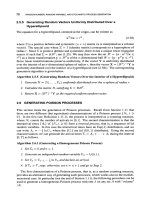
9.4
OTHER RANDOMIZED ALGORITHMS FOR COUNTING
In the previous section we explained how Monte Carlo algorithms can be used for counting
using the importance sampling estimator
(9.5).

In this section we
look
at some alternatives.
In particular, we consider a sequential sampling plan, where the difficult problem of counting
I
X*
I
is decomposed into “easy” problems of counting the number of elements in a sequence
OTHER RANDOMIZED
ALGORITHMS FOR
COUNTING
289
of related sets
XI,.
.
.
,
X,.
A typical procedure for such a decomposition can be written
as follows:
1.
Formulate the counting problem as the problem of estimating the cardinality of some
set
X’.
2. Find sets
Xo,
Xl,.
.
.
,

Xm
such that
IXml
=
I%’\
and
lXol
is
known.
3.
Write
IX*(
=
IXml
as
(9.9)
4.
Develop an efficient estimator
?j3
for each
qj
=
I
Xj
I
/
I
%,
-
1

1
,
resulting in an efficient
estimator,
(9.10)
Algorithms such as based on the sequential sampling estimator (9.10) are sometimes called
randomized algorithms
in the computer literature [22]. We will refer to the notion of a
randomized algorithm as an algorithm that introduces randomness during its execution. In
particular, the standard CE and the PME algorithm below can be viewed as examples of
randomized algorithms.
Remark
9.4.1
(Uniform Sampling)
Finding an efficient estimator for each
qj
=
IXjI/lXj-lI
is the crux of the counting problem. A very simple and powerful idea is
to obtain such an estimator by sampling
uniformly
from the set
gj
=
Xj-1
U
%j.
By
doing
so,

one can simply take the proportion of samples from
gj
that fall in
Xj
as the
estimator for
vj.
For such an estimator to be efficient (have low variance), the subset
Xj
must be relatively “dense” in
q.
In other words
rlj
should not be too small.
is difficult or impos-
sible, one can resort
to
approximate
sampling, for example via the Metropolis-Hastings
Algorithm 6.2.1
;
see in particular Example 6.2.
If exact sampling from the uniform distribution on some set
It
is
shown in [22] and
[23]
that many interesting counting problems can be put into the
setting (9.9). In fact, the CNF SAT counting problem in Section
9.3.1

can be formulated
in this way. Here the objective is to estimate
I%*/
=
1x1
jX*l/l%(
=
1x1
e,
where
1
.XI
is known and
t
can be estimated via importance sampling. Below we give some more
examples.
EXAMPLE
9.4
Independent Sets
Consider a graph
G
=
(V,
E)
with
m
edges and
n
vertices. Our goal is to count
the number of independent node (vertex) sets of the graph. A node set is called

independent
if no two nodes are connected by an edge, that is, if no two nodes are
adjacent; see Figure 9.5 for an illustration of this concept.
290
COUNTING VIA MONTE CARL0
Figure
9.5
The black nodes
form
an independent set, since they are not adjacent to each other.
Consider an arbitrary ordering of the edges. Let
Ej
be the set of the first
j
edges
and let
Gj
=
(V,
Ej)
be the associated subgraph. Note that
G,
=
G
and that
Gj
is
obtained from
G,+l
by removing an edge. Denoting

Xj
the set of independent sets
of
Gj,
we can write
1X.I
=
IX,l
in the form
(9.9).
Here
lX0l
=
2n,
since
Go
has
no edges and thus every subset of
V
is an independent set, including the empty set.
Note that here
Xo
3
Xl
3
.
. .
3
X,
=

X*.
EXAMPLE
9.5
Knapsack Problem
Given items
of
sizes
a.1,
. . .
,
a,
>
0
and a positive integer
b
>
mini
ai,
find the
number
of
vectors
x
=
(XI,.
. .
,x,)
E
(0,l)"
such that

n
The integer
b
represents the size of the knapsack, and
xi
indicates whether or not
item
i
is
put in the knapsack. Let
X*
denote the set of all feasible solutions, that
is, all different combinations of items that can be placed into the knapsack without
exceeding its size. The goal
is
to determine
IX'I.
To put the knapsack problem into the framework
(9.9).
assume without
loss
of
generality that
a1
<
a2
<
.
.
.

<
a,
and define
bj
=
Cz=,
a,,
with
bo
=
0.
Denote
X3
the set of vectors
x
that satisfy
C:=,
ai
xi
<
bj,
and let
m
be the largest integer
such that
b,
,<
b.
Clearly,
X,

=
X'.
Thus,
(9.9)
is established again.
EXAMPLE
9.6
Counting the Permanent
The permanent
of
a general
n
x
n
matrix
A
=
(a,ij)
is defined as
n
(9.1
1)
XCZ
i=l
where
X
is the set of all permutations
x
=
(51,.

.
.
,
x,)
of
(1,.
.
.
,
n).
It is well
known that the calculation of the permanent of a
binary
matrix is equivalent to the
calculation
of
the number
of
perfect matchings in a certain bipartite graph.
A
bipartite
graph
G
=
(V,
E)
is a graph in which the node set
V
is the union of two disjoint sets
V,

and
V2,
and in which each edge joins a node in
V1
to a node in
V2.
A
matching
of
size
m
is a collection
of
m
edges in which each node occurs at most once.
A
perJfect
matching
is a matching of size
n.
OTHER
RANDOMIZED
ALGORITHMS FOR COUNTING
291
To
see the relation between the permanent of a binary matrix
A
=
(aij)
and the

number
of
perfect matchings in a graph, consider the bipartite graph
G,
where
Vl
and
V2
are disjoint copies of
{
1,
.
.
.
,
n}
and
(2,
j)
E
E
if and only if
ail
=
1
for all
i
and
j.
As an example, let

A
be the
3
x
3
matrix
111
A=(:
y).
(9.12)
The corresponding bipartite graph
is
given in Figure
9.6.
The graph has three per-
fect matchings, one
of
which is displayed in the figure.
These correspond to all
permutations
x
for
which the product
n;=,
aiz,
is equal to
1.
34L
3'
Figure

9.6
A
bipartite
graph. The bold edges
form
a
perfect matching.
For a general binary
(n
x
n)
matrix
A,
let
Xj
denote the set of matchings
of
size
j
in the corresponding bipartite graph
G.
Assume that
Xn
is nonempty,
so
that
G
has a perfect matching of nodes
Vl
and

V2.
We are interested in calculating
/.%,I
=
per(A).
Taking into account that
1x11
=
/El,
we obtain the product form
(9.9).
As
a final application of
(9.9),
we consider the general problem
of
counting the number
of elements in the
union
of
some sets
XI,
. .
.
X,.
9.4.1
%*
is
a
Union

of
Some
Sets
Let, as usual,
X
be a finite set of objects, and
let
X*
denote a subset of special objects
that we wish to count. In specific applications
X*
frequently can be written as the
union
of some sets
XI,
. .
.
,
X,,
as illustrated in Figure
9.7.
z
0
0
0
0
0
I
Figure
9.7

Count
the
number
of
points in the
gray
set
%*.
292
COUNTING
VIA
MONTE
CARL0
As
a special case we shall consider the counting problem for a SAT in DNF. Recall
that a DNF formula is a disjunction (logical
OR)
of
clauses
C1
V
C2
V . . . V
C,,
where
each clause
is
a conjunction (logical
AND)
of literals. Let

X
be the set
of
all assignments,
and let
X,
be the subset of all assignments satisfying clause
C,,
j
=
1,
. .
.
,
m.
Denote
by
X'
the set of assignments satisfying
at least
one
of
the clauses
C1,
.
.
.
,
C,,
that is,

X*
=
UF1
X,.
The DNF counting problem is to compute
1
X'I.
It is readily seen that if
a clause
C,
has
nJ
literals, then the number of true assignments is
1
XJ
I
=
2n-nl.
Clearly,
0
5
I
%*I
5
1
XI
=
2"
and, because an assignment can satisfy more than one clause, also
Next, we shall show how to construct a randomized algorithm for this #P-complete

problem. The first step is
to
augment
the state space
X
with an index set
{l,
. .
.
,
m}.
Specifically, define
d=
{(j,x)
:x
E
X,,
j
=
1
, ,
m}.
(9.13)
This set is illustrated in Figure 9.8. In this case we have
m
=
7,
1x1
I
=

3,
IXzl
=
2,
and
so
on.
IX'I
G
Cjn=l
IEJI.
1
2
3
j
1:
m
Figure
9.8
The
sets
d
(formed
by
all
points) and
a'*
(formed
by
the

black
points).
For a fixed
j
we can identify the subset
a'j
=
{(j,x)
:
x
E
X;}
of
a'
with the set
Xj.
In particular, the two sets have the same number
of
elements. Next, we construct a
subset
d*
of
d
with size exactly equal to
(%*(.
This is done by associating with each
assignment in
X'
exactly one pair
(j,

x)
in
a'.
In particular, we can use the pair with the
smallest clause index number, that
is,
we can define
a'*
as
d*={(j,x):x~X~,x$Xj
for
k<j,j=1,
,
m}
In Figure 9.8
d*
is represented by the black points. Note that each element of
X'
is
represented once in
a',
that is, each "column" has exactly one black point.
Since
Id/
=
C,"=,
IX,l
=
Cy=l
2n-nj

is available, we can estimate
IK*I
=
la'*/
=
/dl
l
by estimating
l
=
\a'*\/\d\.
Note that this is a simple application of (9.9). The
ratio
e
can be estimated by generating pairs
uniformly
in
d
and counting how often they
occur in
d*.
It turns
out
that for the union
of
sets, and in particular for the DNF problem,
generating pairs uniformly in
a'
is quite straightforward and can bedone in two stages using
OTHER

RANDOMIZED
ALGORITHMS
FOR COUNTING
293
the composition method. Namely, first choose an index
j,
j
=
1,.
.
.
,
m
with probability
next, choose an assignment
x
uniformly from
Xj.
This can be done by choosing a value
1
or
0
with equal probability and independently for each literal that is
not in clause
j.
The
resulting probability
of
choosing the pair
(j,

x)
can be found via conditioning as
I41
1
1
Id1
I41
14
'
P(J
=
j,x
=
x)
=
P(J
=
j)P(X
=x(
J
=
j)
=
-
-
=
-
which corresponds to the uniform distribution on
d.
The DNF counting algorithm can be

written as follows
[22]
Algorithm
9.4.1
(DNF
Counting Algorithm)
Given is a
DNF
formula with
m
clauses and
n
literals.
I.
Let
Z
=
0.
2.
Fork
=
1
to
N:
i. With probability
pj
0:
I
Xj
1,

choose unformly and randomly an assignment
ii.
rfX
is
not
in any
xi
for
i
<
j,
increase
Z
by
I.
x
E
xj.
3.
Return
(9.14)
as the estimate of the number
1
X*
1
of satisfying assignments.
Note that the ratio
!
=
1d*1/1d1

can be written as
where the subscript
U
indicates that
A
is
drawn uniformly over
d.
Algorithm
9.4.1
counts
the quantity
6
(an estimator of
l),
representing the ratio of the number of accepted samples
2
to the total generated
N,
and then it multiplies
$
by the constant
c,"=,
IXj(
=
Idl.
Note also that Algorithm 9.4.1 can be applied to some other problems involving the union
of
quite arbitrary sets
X,,

j
=
1,.
.
.
,
m.
Next, we present an alternative estimation procedure for
e
in (9.15). Conditioning on
X,
we obtain by the conditioning property (1.1 1):
where
p(X)
=
Pu(Z~A~~.}
I
X)
is
the conditional probability that a uniformly chosen
A
=
(J,
X)
falls in set
d*,
given
X.
For a given element
x

E
.X*,
let
r(x)
denote the
number
of
sets
.Xj
to which
x
belongs. For example, in Figure
9.8
the values for
T(X)
from left to right are
2,
1,
2,
2,
3,
1,.
. . .
Given a particular x, the probability that the
corresponding
(J,
x)
lies in
d*
-

in the figure, this means that the corresponding point in
the columncorresponding to xis black- is simply
l/r(x),
because each of the
T(X)
points
294
COUNTING
VIA
MONTE
CARLO
is chosen uniformly and there is only one representative of
a’*
in each column. In other
words,
p(X)
=
l/r(X).
Hence, if
r(x)
can be calculated for each
x,
one can estimate
e
=
Eu[l/r(X)]
as
Y/N,
with
Y

=
xr=l
&.
By doing
so,
we obtain the estimator
(9.16)
Note that in contrast to (9.14) the estimator in (9.16) avoids the acceptance-rejection step.
Both
I@?
and are unbiased estimators of
I%*/,
but the latter has the smaller vari-
ance of the two, because
it
is obtained by conditioning;
see
the conditional Monte Carlo
Algorithm 5.4.1.
Both
IX*l
and
IZ*I
can be viewed as importance sampling estimators of the form
(9.4). We shall show it for the latter. Namely, let
g(x)
=
T(x)/c,
x
E

X’,
where
c
is
a normalization constant, that is,
c
=
CxEz.
T(X)
=
EL,
/Xi/.
Then, applying (9.3,
with
d*
and
d
instead
of
X’
and
X,
gives the estimator
-
-
which is exactly
I
X*
I.
As mentioned, sampling from the importance sampling pdf

g(x)
is
done via the composition method without explicitly resorting to
T(x).
Namely, by selecting
(J,
X)
uniformly over
d,
we have
T(X)
P(X
=
x)
=
-
=
g(x), x
E
X*
1-4
We shall show below that the DNF Counting Algorithm 9.4.1 possesses some nice com-
plexity properties.
9.4.2
Complexity
of
Randomized Algorithms: FPRAS and FPAUS
A randomized algorithm is said to give an
(E,
6)-upproximution

of a parameter
z
if its output
2
satisfies
P(lZ
-
21
<
€2)
2
1
-
6,
(9.17)
that is, the “relative error”
12
-
zI/z
of
the approximation
Z
lies with high probability
(>
1
-
6)
below some small number
E.
One of the main tools in proving (9.17) for various randomized algorithms is the so-called

Chernoffbound,
which states that for any random variable
Y
and any number
a
P(Y
<
a)
<
mineea ~[e-’~]
.
(9.18)
Namely, for any fixed
a
and
0
>
0,
define the functions
Hl(z)
=
I{z(a)
and
H~(z)
=
es(a-z). Then, clearly,
Hl(z)
<
H~(z)
for all

z.
As a consequence, for any
8,
0>0
P(Y
<
a,)
=
E[H~(Y)]
<
E[H~(Y)]
=
eea
i~[e-~~]
.
The bound (9.18) now follows by taking the smallest such
8.
An important application is
the following.
OTHER
RANDOMIZED
ALGORITHMS FOR
COUNTING
295
Theorem
9.4.1
Let
XI,
. . .
,

X,,
be iid
Ber(p)
random variables. Then their sample mean
provides an
(E,
6)-approximation for
p,
that is,
(9.19)
provided that
n
2
3
ln(2/6)/(p~~).
Proof
IE[e-BX1]n
=
(1
-
p
+
pee),,, the Chemoff bound gives
Let
Y
=
XI
+

+

X,,
and
l?~
=
P(Y
<
(1
-
~)np).
Because E[e-eY]
=
eL
,<
een~(l-~)
(1
-P+Pee)n,
(9.20)
for any
8
>
0.
By direct differentiation we find that the optimal
8’
(giving the smallest
upper bound) is
It is not difficult to verify (see Problem 9.1) that by substituting
6’
=
8’
in

the
right-hand
side of (9.20) and taking the logarithms on both sides,
In(!,)
can be upper-bounded by
np
h(p,
E).
where
h(p,
E)
is given by
h(~,p)
=

In
(
1
+
-
l:p)
+
(1
-
E)B*
.
P
(9.21)
For fixed
0

<
E
<
1,
the function
h(p,
E)
is monotonically decreasing
in
p,
0
<
p
<
1.
Namely,
since
-y
+
In(1
+
y)
<
0
for any
y
>
0.
It follows that
And therefore,

e,
<
exp
(-$)
Similarly, Chernoff’s bound provides the following upper bound for
Cu
=
P(Y
2
(1
+
E)np)
=
P(-Y
<
-(1
+
E)np):
(9.22)
for all
0
<
E
<
1;
see Problem 9.2. In particular,
l?,
+
Cu
<

2
exp(-np~~/3). Combining
these results gives
np
~~13
P(IY
-
npl
<
np~)
=
1
-
e,
-
e,
2
1
-
2e
,
so
that by choosing
n
2
3
ln(2/6)/(p&’),
the
above probability
is

guaranteed to be greater
than or equal to
1
-
6.
0
296
COUNTING
VIA
MONTE
CARLO
Definition 9.4.1 (FPRAS)
A randomized algorithm is said to provide a
fullypolynomial
randomized approximation scheme (FPRAS)
if, for any input vector
x
and any parameters
E
>
0
and
0
<
6
<
1,
the algorithm outputs an
(E,
6)-approximation to the desired quantity

Z(X)
in time that is polynomial in
E-~,
In
6-'
and the size
n
of the input vector
x.
Thus, the sample mean in Theorem 9.4.1 provides an FPRAS for estimating
p.
Note that
the input vector
x
consists of the Bernoulli variables
XI,
.
. . ,
X,.
Below we present a theorem [22] stating that Algorithm 9.4.1 provides an
FPRAS
for
counting the number of satisfying assignments in
a
DNF formula. Its proof is based
on
the
fact that
d*
is relatively

dense
in
d.
Specifically, it uses the fact that for the union of
sets
I
=
ld*l/ldl
2
l/m,
which follows directly from the fact that each assignment can
satisfy at most
m
clauses.
Theorem 9.4.2 (DNF Counting Theorem)
The DNF counting Algorithm
9.4.1
is an
FPRAS, provided that
N
2
3m
ln(2/6)/~~.
Proof
Step
2
of Algorithm 9.4.1 chooses an element uniformly from
d.
The probability
that this element belongs to

d*
is at least
l/m.
Choose
3m
2
N=-ln-
€2
6
'
(9.23)
where
E
>
0
and 6
>
0.
Then
N
is polynomial in
m,
and
In
i,
and the processing
time of each sample is polynomial in
m.
By Theorem 9.4.1 we find that with the number
of samples

N
as in (9.23), the quantity
Z/N
(see Algorithm 9.4.1) provides an
(E,
6)-
approximation
to
e
and thus
IX.1
provides an
(E,
6)-approximation to
I%-* I.
0

As observed at the beginning of this section, there exists a fundamental connection
between
uniform sampling
from some set
X
(such as the set
d
for the DNF counting
problem) and
counting
the number of elements of interest in this set
[
1,

221. Since, as we
mentioned, exact uniform sampling is not always feasible, MCMC techniques are often
used
to
sample
approximafely
from a uniform distribution.
Let
Z
be the random output of a sampling algorithm on a finite sample space
X.
We say
that the sampling algorithm generates an
E-uniform sample
from
2-
if, for any
c
X,
llF(Z
E
9)
-
<
E
1x1
(9.24)
Definition 9.4.2 (FPAUS)
A
sampling algorithm is called a

fullypolynomial almost uni-
form sampler (FPAUS)
if, given an input vector
x
and a parameter
E
>
0,
the algorithm
generates an &-uniform sample from
X(x)
and runs in time that is polynomial in
In€-I
and the size
of
the input vector
x.
EXAMPLE
9.7
FPAUS
for
Independent Sets: Example 9.4 Continued
An FPAUS for independent sets takes as input a graph
G
=
(V,
E)
and a parameter
E
>

0.
The sample space
X
consists of all independent sets in
G,
with the output
being an E-uniform sample from
%.
The time required to produce such an E-uniform
sample should be polynomial in the size of the graph and
In
E-~.
The final goal is to
prove that given an FPAUS, one can construct a corresponding
FPRAS.
Such a proof
is based on the product formula (9.9) and is given in Theorem 10.5 of [22].
For the knapsack problem, it can be shown that there is an
FPRAS
provided
that there
exists an FPAUS;
see
also Exercise 10.6 of
[22].
However, the existence of such a method
is still an open problem
[
151.
MINXENT

AND
PARAMETRIC
MINXENT
297
9.4.3
FPRAS
for
SATs in CNF
Next, we shall show that all the above results obtained
so
far for SATs in the DNF also apply
to SATs in the CNF. In particular, the proof
of
FPRAS and FPAUS
is
simple and therefore
quite surprising. It
is
based on De Morgan’s law,
(n.;>’
=
u
.x,c
and
(u.;)‘
=
n
.x,c.
Thus, if the
{

Zi)
are subsets of some set
Z,
then
Iu
4‘1
(9.25)
(9.26)
In particular, consider a CNF SAT counting problem and let
Xi
be the set of all assignments
that satisfy the i-th clause,
Ci,
i
=
1,
. . .
,
m.
Recall that
Ci
is of the form
zil
Vzi2
V.
.
’Vzik.
The set of assignments satisfying
all
clauses is

X*
=
nZ,.
In view
of
(9.26),
to count
Z*
one could instead count the number of elements in
LIZi‘.
Now
ZiC
is the set
of
all
assignments that satisfy the clause
Zil
A
Ziz
A
. .
A
F,k.
Thus, the problem is translated
into a DNF SAT counting problem.
As an example, consider the CNF SAT counting problem with clause matrix
A=
(-:
-;
:)

.
In this case
Z*
comprises three assignments, namely,
(l,O,O),
(1,1,0),
and
(II 1,l).
Consider next the DNF SAT counting problem with clause matrix
-A.
Then the set of assignments that satisfy at least one clause for this problem
is
{(O,O,
0),
(O,O,
l),
(0,1,0), (0,1,
l),
(l,O,
l)},
which is exactly the complement of
Z*.
Since the DNF SAT counting problem can be solved via an FPRAS, and any CNF SAT
counting problem can be straightforwardly translated into the former problem, an
FPRAS
can be derived for the CNF SAT counting problem.
-1
0
-1
9.5

MINXENT AND PARAMETRIC MINXENT
This section deals with the parametric MinxEnt (PME) method for estimating rare-event
probabilities and counting, which is based on the MinxEnt method. Below we present some
background on the MinxEnt method.
9.5.1
The MinxEnt Method
In the standard CE method for rare-event simulation, the importance sampling density for
es-
timating[
=
Pf(S(X)
2
y)
is restricted tosomeparametricfamily, say
{f(.;
v),
v
E
Y),
and the optimal density
f(.;
v’)
is found as the solution to theparametric CE minimization
program
(8.3).
In contrast to CE, we present below a nonparametric method called the
MinxEnt
method. The idea
is
to minimize the CE distance to

g*
over
all
pdfs rather than
over
{f(.;v), v
E
Y).
However, the program min,
D(glg*)
is void of meaning, since
the minimum (zero) is attained at the unknown
g
=
9”.
A more useful approach is to first
specify a prior density
h,
which conveys the available information on the “target”
g*,
and
then choose the “instrumental” pdf
g
as close as possible to
h,
subject to certain constraints
298
COUNTING
VIA
MONTE CARL0

on
g.
If no prior information on the target
g*
is known, the prior
h
is
simply taken to
be
a
constant, corresponding to the uniform distribution (continuous or discrete). This leads to
the following minimization framework [2], [3], and
[
171:
ming
D(g,
h)
=
min,
s
In
g(x) dx
=
min
s.t.
J
S,(X) g(x)
dx
=
E,[S,(X)]

=
yz,
i
=
1,.
.
.
,
rn
,
I
(9.27)
Jg(x)dx=
1.
Here
g
and
h
are n-dimensional pdfs,
Si
(x),
i
=
1,
.
.
.
,
m,
are given functions, and

x
is
an
n-dimensional vector. The program
(PO)
is Kullback’s minimum cross-entropy (MinxEnt)
program. Note that this is a
conva
functional optimization problem, because the objective
function is a convex function of
g,
and the constraints are affine in
g.
g(x) Ing(x) dx
+
constant,
so
that the
minimization of
D(g,
h)
in
(PO)
can be replaced with the maximization of
If the prior
h
is constant, then
D(g,
h)
=

Wg)
=
-
g(x) Ing(x) dx
=
-E,bg(X)l
I
(9.28)
where
X(g)
is the Shannon entropy; see
(1.52).
(Here we use a different notation to
emphasize the dependence on
9.)
The corresponding program is Jaynes’ MuxEnt program
[
131. Note that the former minimizes the Kullback-Leibler cross-entropy, while the latter
maximizes the Shannon entropy
[17].
In
typical counting and combinatorial optimization problems
IL
is chosen as an n-
dimensional pdf with uniformly distributed marginals.
For example, in the SAT count-
ing problem, we assume that each component of the n-dimensional random vector
X
is
Ber(

1/2)
distributed. While estimating rare events in stochastic models, like queueing
models,
h
is the fixed underlying pdf. For example, in the
M/M/1
queue
h
would be a
two-dimensional pdf with independent marginals, where the first marginal is the interarrival
Exp(X)
pdf and the second
is
the service
Exp(p)
pdf.
The MinxEnt program, which presents a constrained functional optimization problem,
can be solved via Lagrange multipliers. The solution for the discrete case is derived in
Example 1.20 on page 39. A similar solution can be derived, for example, via calculus
of
variations [2], for the general case. In particular, the solution of the MinxEnt problem is
s
(9.29)
where
Xi,
i
=
1,
. .
.

,
7n
are obtained from the solution of the following system of equations:
where
X
-
h(x).
Note that
g(x)
can be written as
(9.31)
MINXENT
AND
PARAMETRIC
MINXENT
299
where
(9.32)
is
the
normalization constant. Note also that
g(x)
is a density function;
in
particular,
g(x)
2
0.
Consider the MinxEnt program
(PO)

with a single constraint, that is,
min,
D(g,
h)
=
min,
IE,
[In
H]
J
g(s)
dx
=
1
s.t.
E,(S(X)]
=
y
,
In this case (9.29) and (9.30) reduce to
and
(9.33)
(9.34)
(9.35)
respectively.
function, that is,
In the particular case where
S(x),
x
=

(xl,
. .
.
,
5,)
is a coordinatewise separable
S(X)
=
c
Sib,)
(9.36)
and the components
X,,
i
=
1,
.
. .
,
n
of the random vector
X
are independent under
h(x)
=
h(x1)
.
. .
h(xTL),
the joint pdf

g(x)
in
(9.34) reduces to the
product ofmarginal
pdfs.
In particular, the i-th component of
g(x)
can be written as
n
2=1
(9.37)
Remark
9.5.1
(The MinxEnt Program with Inequality Constraints)
It is not difficult
to extend the MinxEnt program to contain
inequality
constraints. Suppose that the fol-
lowing
M
inequality constraints are added to the MinxEnt program (9.27):
E,[S,(X)]
by,,
i=m+l,
,
m+M.
The solution of this MinxEnt program is given by
h(x)
exp
{

CE:~
s,(x)}
g(x)
=
(9.38)
IEh
[exp
{
c::”
Sz(X)}]
’
where the Lagrange multipliers
X1,
. . .
,
Xm+~
are the solutions to the dual convex opti-
mization problem
subject to:
Xi
2
0,
i
=
m
+
1,.
.
.
,

m
+
M.
300
COUNTING
VIA
MONTE
CARL0
Thus, only the Lagrange multipliers corresponding to an inequality must be constrained
from below by zero. Similar to (1.87), this can be solved in two steps, where
p
can
be determined explicitly as a normalization constant but the
{Xi}
have to be determined
numerically.
In the special case of a single inequality constraint (that is,
m
=
0
and
M
=
l),
the dual
program can be solved directly (see also Problem
9.9),
yielding the following solution:
0
ifEh[S(X)]

b
y
A={
A*
ifEh[S(X)]
<
y
,
where
A'
is obtained from
(9.35).
That is, if Eh[S(X)]
<
7,
then the inequality MinxEnt
solution agrees with the equality MinxEnt solution; otherwise, the optimal sampling pdf
remains the prior
h.
Remark
9.5.2
It is well known
[9]
that the optimal solution of the single-dimensional
single-constrained MinxEnt program
(9.33)
coincides with the celebrated optimal
expo-
nential change
of

measure (ECM). Note that normally in a multidimensional ECM one
twists each component separately, using possibly different twisting parameters. In contrast,
the optimal solution to the MinxEnt program (see
(9.37))
is parameterized by a single-
dimensional parameter
A.
If not otherwise stated, we consider below only the single-constrained case
(9.33).
Like
in the standard CE method one can also use a multilevel approach, where a sequence of
instrumentals
{gt}
and levels
{yt}
is used. Starting with
go
=
f
and always taking prior
h
=
j',
we determine
yt
and
gt
as follows:
1.
Update

Yt
as
Yt
=
Eg,[S(X)
I
S(X)
b
stl
>
where
qt
is the
(1
-
e)-quantile of S(X) under
gt-
1.
2.
Update
gt
as the solution to the above MinxEnt program for level
yt
rather than
y.
The updating formula for
yt
is based on the constraint Eg[S(X)]
=
y

in the MinxEnt pro-
gram. However, instead of simply updating as
yt
=
lEgt_l
[S(X)], we take the expectation
of S(X) with respect to
gt-1
conditionalupon S(X) being greater than its
(1
-
Q)
quantile,
here denoted as
qt.
In contrast, in the standard CE method the level
yt
is simply updated
as
st.
Note that each
gt
is completely determined by its Lagrange multiplier, say
At,
which is
the solution
to
(9.35)
with
yt

instead
of
y.
In practice, both
yt
and
At
have to be replaced
by their stochastic counterparts
Tt
and
At,
respectively. Specifically,
yt
can be estimated
from a random sample
XI,.
.
.
,
XN
of
yt-1
as the average of the
Ne
=
[(l
-
Q)N~
elite

sample performances:
A
(9.39)
where
S(i)
denotes the i-th order-statistics of the sequence S(Xl),
.
.
.
,
~(XN). And
At
can be estimated by solving, with respect to
A,
the stochastic counterpart of
(9.33,
which
is
(9.40)
MINXENT
AND
PARAMETRIC
MINXENT
301
9.5.2
Rare-Event Probability Estimation Using PME
The above MinxEnt approach has limited applications
[25],
since it requires sampling from
the complex multidimensional pdf

g(x)
of
X.
For
this reason we shall consider in this
section a modified version of MinxEnt, which is based on the marginal distributions of
g(x).
The modified version
is
called theparametric MinxEnt (PME) method. We focus on
the estimation of the rare-event probability
where we assume for simplicity that
X
=
(XI,.
. .
X,)
is a binary random vector with
independent components with probabilities
u
=
(211,.
.
.
u,),
that is,
X
N
Ber(u).
Let

f(x;
u)
denote the corresponding discrete pdf. We can estimate
d
via the likelihood ratio
estimator as
(9.41)
where
XI,
,
.
.
,
XN
is a random sample from
Ber(p),
for some probability vector
p.
typi-
cally different from
u.
The question is how to obtain a
p
that gives a low variance for the
estimator
e^.
If
e
is related to a counting problem, as in
(9.Q

the same
p
can be used in
(9.5)
to estimate
I%*J.
Let
g(x)
in
(9.34)
be the optimal MinxEnt solution for this estimation problem. By
summing
g(x)
over all
xi7
i
#
j, we obtain the marginal pdf for the j-th component. In
particular, let
g(x)
be the MinxEnt pdf, as in
(9.34),
and
h(x)
=
f
(x;
u),
the prior pdf;
then under

g
we have
X,
N
Ber(p,),
with
so
that
E,
[x,
,
pj
=
,
J
=
1,
,
n,
E,
[eA
S(X)]
(9.42)
with
X
satisfying
(9.35).
Note that these
{pj}
will form our importance sampling parameter

vector
p.
Observe also that
(9.42)
was extensively used in
[25]
for updating the parameter
vector
p
in rare-event estimation and for combinatorial optimization problems. Finally, it is
crucial to recognize that
(9.42)
is
similar to the corresponding
CE
formula
(see
also
(5.67))
(9.43)
with one main difference: the indicator function
I{s(x)b7}
in the
CE
formula is replaced
by
exp
{
X
S(X)}.

We shall call
pj
in
(9.42)
the optimal PMEparameter and consider it as
an alternative to
(9.43).
Remark
9.5.3
(PME for Exponential Families)
The PME updating formula
(9.42)
can
be generalized to hold for any exponential family parameterized by the mean in the same
way that the CE updating formula
(9.43)
holds for such families. More specifically, suppose
that under prior
h(x)
=
f
(x;
u)
the random vector
X
=
(XI,.
.
.
,

X,)
has independent
components, and that each
X,
is distributed according to some one-parameter exponential
family
fl(zE;
ul)
that is parameterized by its mean
-
thus,
lEh[X,]
=
Eu[X,]
=
u,,
with
302
COUNTING VIA MONTE CARL0
u
=
(ul,
. . .
,
un).
The expectation of
X,
under the MinxEnt solution is (in the continuous
case)
Let

v
=
(711,.
.
.
,
7Jn)
be another parameter vector for the exponential family. Then the
above analysis suggests carrying out importance sampling using
vj
equal to
Eg[Xj]
given
in
(9.44).
Another way of looking at this is that
v
is chosen such that the Kullback-Leibler dis-
tance from the Boltzmann-like distribution
b(x)
0:
f(x;
u)
eXS(X)
to
f(x;
v)
is minimized.
Namely, minimizing
D(b,

f(.;
v))
with respect to
v
is equivalent to maximizing
1
h(x)
ex
In
f(x;
v)
dx
=
E,[eX
In
f(X;
v)]
,
which (see
(A.15)
in Section
A.3
of the Appendix) leads directly to the updating formula
(9.44).
Compare this with the standard CE method, where the Kullback-Leibler distance
from
g*
(x)
0:
f(x;

U)I~S(~)~~~
to
f(x;
v)
is minimized instead.
Note that
1.
For
a
separable function
S(x)
MinxEnt
reduces
to PME. Recall that in this case the
optimal joint pdf presents a product of marginal pdfs. Thus, PME is well suited for
separable functions, such as those occumng in SATs (see
(9.7)).
However, it follows
from Remark
9.5.2
that, even for separable functions, PME is
essentially different
from ECM.
2.
Similar to CE, the optimal PME updating
pt
and its estimators can be obtained
analytically and on-line.
3.
One does not need to resort to the MinxEnt program and to its joint pdf in order to

derive the optimal parameters
p:.
4.
The optimal
A*
is the same in both MinxEnt and PME.
5.
Sampling from the marginal discrete pdf with the optimal parameters
{pf}
is easy
and is similar to CE.
PME is well suited for separable functions (see item
1
above) and, it will turn out, also
for block-separable functions, such as those that occur in the SAT problem (see
(9.7)).
Here
block-separable
means a function of the form
S(X)
=
Sl(Y1)
+
”‘
+
Sm(Yrn)
,
where each vector
yi
depends on at most

T
<
n
variables in
(21,.
. .
,
zn}.
One might wonder why the PME parameter in
(9.42)
would be preferable to the standard
CE one in
(9.43).
The answer lies in the fact that in complex simulation-based models
the PME optimal parameters
p
and
X
are typically not available analytically and need to
be estimated via Monte Carlo simulation. It turns out
-
this is discussed below
-
that
for separable and block-separable function the corresponding estimator of
(9.42)
can have
a significantly lower variance than the estimator of
(9.43).
This, in turn, means that the

MINXENT
AND
PARAMETRIC
MINXENT
303
-
variance of the estimator
e?
and for a counting problem the variance of estimator
lX*l,
will
be significantly reduced.
For the estimation of the PME optimal parameters
p
and
X
one can use, as in the CE and
MinxEnt methods, a dynamic (multilevel) approach in which the estimates are determined
iteratively. This leads to the following updating formula for
pj
at the t-th iteration:
k=l
where
it
is obtained from the solution of (9.40) and
W
denotes, as usual, the likelihood
ratio.
Note that
-l/Xt

can be viewed as a temperature parameter. In contrast to simulated
annealing, the temperature is chosen here optimally in the CE sense rather than heuristically.
Also,
in contrast to CE, where only the elite sample is used while updating
p,
in PME (see
(9.45)) the entire sample is used.
We explain via a number of examples why the PME updating formula (9.45) can be
much more stable than its CE counterpart,
N
k=l
Ft,j
=
C
'{s(xk)>Ft)
w(xk;
u,
6t-l)
k=l
The key difference is that the number of product terms in
W
for CE is
always
n
(the size
of the problem):
irrespective of the form of
S(x),
whereas the PME estimator (9.45) for separable or block-
separable functions can be readily modified such that the number of product terms of the

likelihood ratio is much smaller than
n.
EXAMPLE93
Consider a separable sample function, that is:
n
S(X)
=
CSj(Zj)
.
j=1
Then (9.42) reduces to
304
COUNTING VIA MONTE CARL0
which can be estimated via importance sampling as
N
(9.46)
-
k=l
pt,J
=
N
A
exp{%
sj
(Xkj
)
}
wj
(Xkj
;

21.1
Pl-
1,~)
k=l
While both (9.45) and (9.46) represent unbiased estimators of
p,,
the former involves
the highly unstable likelihood ratio
W(X)
=
n,"=,
W,(X,)
with respect to the
n-dimensional vector
X,
whereas the latter involves only the likelihood ratio with
respect to the one-dimensional variable
X,.
As
a consequence, the estimator
in
(9.46)
generally will have a much smaller variance than the one in (9.45).
EXAMPLE9.9
Consider next a block-separable function
S(x)
of the form
n-
1
~(x)

=
Csj(sj,zj+l)
.
J=1
Suppose we want to estimate
p2.
Consider first the case where
S3
=
0.
Define
J
=
{
1,2,3}
and
=
(4,
.
. .
,
TI}.
Let
us
denote by
x
J
the vector with components
{
s3,

j
E
J}
and similar for
XJ.
We can now write
S(x)
as
s(x)
=
sJ(xJ)
f
sJ(xJ)
,
(9.47)
with
SJ(XJ)
=
&(Xl,Xz)
+
s2(x2,x3)
and
Sj(X,-)
=
CyL:
S3(X3,X3+1)
being
independent.
In this case, according to (9.42), the component
p,,

j
=
2
of
p
can be updated according to
(9.48)
-
-
[xJ
exP{ASJ(XJ)}]
'UJ
[exp
sJ(xJ)}]
'
which can be estimated via importance sampling as
N
cxkj
exP{%
sJ(xkJ)}
WJ(XkJ;
U16t-1)
,
(9.49)
-
k=l
pt>,
=
N
xexP{%

s(xkJ)}
WJ(XkJ;
U,6t-1)
k=
1
with
WJ
the corresponding likelihood ratio, which now only has two product terms.
Thus, for large
TI,
the estimator in (9.49) typically has a much smaller variance than
the one in (9.45)
Suppose next that
S3
does not vanish,
so
that
SJ(XJ)
and
SJ(XJ)
are depen-
dent. Then, obviously, (9.45) is no longer valid. Nevertheless, for block-separable
functions, this formula can still be used as an approximation to the true updating
formula (9.42). In this case the estimator based on (9.45) may contain some bias, but