SIMULATION AND THE MONTE CARLO METHOD Episode 12 pptx
Bạn đang xem bản rút gọn của tài liệu. Xem và tải ngay bản đầy đủ của tài liệu tại đây (1.16 MB, 30 trang )
31 0
COUNTING
VIA
MONTE
CARL0
Table
9.7
A
=
(75
x
325)
and
N
=
100,000.
Performance
of
the PME algorithm
for
the random
3-SAT
with the clause matrix
t
6
7
8
9
10
11
12
13
14
15
16
-
Min
Mean Max
0.00 0.00 0.00
382.08 1818.15
0.00
1349.59 3152.26
0.00
1397.32 2767.18 525.40
1375.68 1828.1
1
878.00
434.95
1776.47 1341.54
374.64 1423.99
1340.12
392.17 1441.19 1356.97
397.13 1466.46 1358.02
384.37 1419.97 1354.32
377.75 1424.07 1320.23
IF1
Found
Mean Max Min
0.00
0 0
4.70 35
0
110.30 373
0
467.70 1089 42
859.50 1237 231
153.70 1268 910
244.90 1284 1180
273.10
1290 1248
277.30 1291 1260
277.10 1296 1258
271.90 1284 1251
PV
0.0000
0.0000
0.001
8
0.0369
0.1
143
0.2020
0.2529
0.2770
0.28 16
0.2832
0.2870
RE
NaN
1.7765
0.8089
0.4356
0.1755
0.0880
0.0195
0.0207
0.0250
0.0
166
0.0258
Figure
9.10
matrix
A
=
(75
x
325)
and
N
=
100,000.
vpical dynamics
of
the PME algorithm
for
the random
3-SAT
problem with the clause
-O
0.5-
0
10
20
30
40
50
60
70
-N
0.5
0
10
20
30
40
50
60
70
-w
0.;;
0
10
20
30
40
50
60
70
Y
10
20
30
40
50
60
70
10
20
30
40
50
60
70
10
20
30
60
10
20
30
40
50
60
70
-
f
o.;"]
0
10
20
30
40
50
60
70
"
10
20
30
40
50
60
70
"
10
20
30
40
50
60
70
PROBLEMS
311
PROBLEMS
9.1
Prove the upper bound
(9.21).
9.2
Prove the upper bound
(9.22).
9.3
Consider Problem
8.9.
Implement and run a PME algorithm on this synthetic max-
cut problem for a network with
n
=
400
nodes, with
m
=
200.
Compare with the CE
algorithm.
9.4
Let
{ A,}
be an arbitrary collection of subsets of some finite set
X.
Show that
This is the useful
inclusion-exclusion
principle.
9.5
A
famous problem in combinatorics is the
distinct representatives
problem, which
is formulated as follows. Given a set
d
and subsets
dl,
.
. . ,
dn
of
d,
is there a vector
x
=
(z1,
. .
.
,
2,)
such that
z,
E
d,
for each
i
=
1,
. . .
,
nand the
{xi}
are all distinct (that
is,
z,
#
z3
if
i
#
j)?
a)
Suppose, for example, that
d
=
{
1,2,3,4,5},
d1
=
{
1;
2,5},
d2
=
{
1,4},
~$3
=
{3,5},
dd
=
{3,4},
and
ds
=
{
1).
Count the total number of distinct
representatives.
b)
Argue why the total number of distinct representatives in the above problem is
equal to the
permanent
of the following matrix
A.
9.6
Let
XI,
.
.
.
,
X,
be independent random variables,each with marginal pdf
f.
Suppose
we wish to estimate
!
=
Pj
(XI
+
.
. .
+
X,
2
y)
using MinxEnt. For the prior pdf, one
could choose
h(x)
=
f(zl)f(zz).
.
.
f(z,),
that is, the joint pdf. We consider only a
single constraint in the MinxEnt program, namely,
S(x)
=
x1
+
. .
.
+
2,.
As in
(9.34),
the solution to this program is given by
where
c
=
l/lE~[eXS(X)]
=
(lE~[e'~])-" is a normalization constant and
X
satisfies
(9.35).
Show that the new marginal pdfs are obtained from the old ones by an
exponential twist,
with twisting parameter
-X;
see also
(A.13).
9.7
Problem
9.6
can be generalized to the case where
S(x)
is a coordinatewise separa-
ble function, as in
(9.36),
and the components
{Xi}
are independent under the prior pdf
h(x).
Show that also in this case the components under the optimal MinxEnt pdf
g(x)
are
independent and determine the marginal pdfs.
312
COUNTING
VIA
MONTE
CARL0
9.8
Let
X
be the set of permutations
x
=
("1,
. . .
,
z,)
of the numbers
1,.
. .
,
n,
and let
n
S(x)
=
c
j
"j
(9.5 1)
3=1
Let
X*
=
{x
:
S(x)
2
y},
where
y
is chosen such that
IX'I
is very small relative to
Implement a randomized algorithm to estimate
I
X
*
I
based on (9.9), using
Xj
=
{
x
:
S(x)
2
yj},
for some sequence of
{yj}
with
0
=
yo
<
y1
<
.
.
.
<
yT
=
y.
Estimate each
quantity
Pu(X
E
Xk
I
X
E
Xk-1).
using the Metropolis-Hastings algorithm for drawing
from the uniform distribution on
Xk-1.
Define two permutations
x
and
y
as neighbors if
one can be obtained from the other by swapping two indices, for example
(1,2,3,4,5)
and
9.9
Write the Lagrangian dual problem for the MinxEnt problem with constraints in
Remark 9.5.1.
1x1
=
n!.
(2,L
3,4,5).
Further
Reading
For good references on #P-complete problems with emphasis
on
SAT problems see [2 1,221.
The counting class #P was defined by Valiant [29]. The
FPRAS
for counting SATs in DNF
is due to Karp and Luby
[
181, who also give the definition of FPRAS. The first
FPRAS
for counting the volume of a convex body was given by Dyer et al.
[
101. See also [8] for
a general introduction to random and nonrandom algorithms. Randomized algorithms for
approximating the solutions of some well-known counting #P-complete problems and their
relation to MCMC are treated in
[I
1, 14, 22, 23, 281. Bayati and Saberi [I] propose an
efficient importance sampling algorithm for generating graphs uniformly at random. Chen
et al. [7] discuss the efficient estimation, via sequential importance sampling, of the number
of
0-1
tables with fixed row and column sums. Blanchet [4] provides the first importance
sampling estimator with bounded relative error for this problem. Roberts and Kroese [24]
count the number of paths in arbitrary graphs using importance sampling.
Since the pioneering work of Shannon [27] and Kullback [19], the relationship between
statistics and information theory has become a fertile area of research. The work of Kapur
and Kesavan, such as [16, 171, has provided great impetus to the study of entropic princi-
ples in statistics. Rubinstein [25] introduced the idea of updating the probability vector for
combinatorial optimization problems and rare events using the marginals of the MinxEnt
distribution. The above PME algorithms for counting and combinatorial optimization prob-
lems present straightforward modifications of the ones given in [26]. For some fundamental
contributions to MinxEnt see [2, 31. In
[5,
61 a powerful generalization and unification of
the ideas behind the MinxEnt and
CE
methods is presented under the name
generalized
cross-entropy
(GCE).
REFERENCES
1.
M.
Bayati
and
A.
Saberi. Fast generation
of
random graphs
via
sequential importance sampling.
Manuscript, Stanford University,
2006.
2.
A.
Ben-Tal,
D.
E.
Brown,
and
R.
L.
Smith.
Relative
entopy
and
the convergence of
the
posterior
and
empirical
distributions
under incomplete
and
conflicting
information. Manuscript, University
of
Michigan,
1988.
REFERENCES
313
3. A. Ben-Tal and M. Teboulle. Penalty functions and duality in stochastic programming via
q5
divergence functionals.
Mathematics of Operations Research,
12:224-240, 1987.
4.
J.
Blanchet. Importance sampling and efficient counting of 0-1 contingency tables. In
Valuetools
'06:
Proceedings of the 1st International Conference
on
Performance Evaluation Methodolgies
and Tools,
page 20. ACM Press, New York, 2006.
Stochastic Methods for Optimization and Machine Learning.
ePrintsUQ,
BSc (Hons) Thesis, Department of Mathematics,
School of Physical Sciences, The University of Queensland, 2005.
6.
Z.
I.
Botev, D. P. Kroese, and T. Taimre. Generalized cross-entropy methods for rare-event sim-
ulation and optimization.
Simulation: Transactions of the Society for Modeling and Simulation
International,
2007. In press.
7.
Y. Chen, P. Diaconis,
S.
P. Holmes, and J. Liu. Sequential Monte Carlo method for statistical
analysis of tables.
Journal ofthe American Statistical Association,
100: 109-120, 2005.
8. T. H. Cormen, C. E. Leiserson,
R.
L. Rivest, and C. Stein.
Introduction to Algorithms.
MIT
Press and McGraw-Hill, 2nd edition, 2001.
9. T. M. Cover and J. A. Thomas.
Elements of Information Theory.
John Wiley
&
Sons, New
York,
1991.
10.
M. Dyer, A. Frieze, and R. Kannan. A random polynomial-time algorithm for approximation
11. C. P. Gomes and B. Selman. Satisfied with physics.
Science,
pages 784-785, 2002.
12. J. Gu, P. W. Purdom,
J.
Franco, and B. W. Wah. Algorithms for the satisfiability (SAT) problem:
5.
2.
I.
Botev.
the volume of convex bodies.
Journal ofthe ACM,
38:l-17, 1991.
A survey. In
Satisfi ability Problem: Theory andApplications,
volume 35 of DIMACS Series in
Discrete Mathematics. American Mathematical Society, 1996.
13. E.
T.
Jaynes.
Probability Theory: The Logicofscience.
Cambridge University Press, Cambridge,
2003.
14. M. Jermm.
Counting, Sampling and Integrating: Algorithms and Complexity.
Birkhauser
Verlag, Basel, 2003.
15. M. Jermm and A. Sinclair.
Approximation Algorithms for NP-hard Problems,
chapter
:
The
Markov chain Monte Carlo Method: An approach to approximate counting and integration.
PWS, 1996.
16. J.
N.
Kapur and
H.
K. Kesavan. Thegeneralized maximum entropy principle.
IEEE Transactions
on
Systems, Man, and Cybernetics,
19:1042-1052, 1989.
17. J. N. Kapur and H. K. Kesavan.
Entropy Optimization Principles with Applications.
Academic
Press, New York, 1992.
18. R. M. Karp and M. Luby. Monte Carlo algorithms for enumeration and reliability problems. In
Proceedings of the 24-th IEEE Annual Symposium
on
Foundations of Computer Science,
pages
56-64,
Tucson, 1983.
19.
S.
Kullback.
Information Theory and Statistics.
John Wiley
&
Sons, New York, 1959.
20. J.
S.
Liu.
Monte Carlo Strategies
in
Scientij c Computing.
Springer-Verlag. New York, 2001.
21. M. MCzard and Andrea Montanan.
Constraint Satisfaction Networks in Physics and Computa-
22. M. Mitzenmacher and E. Upfal.
Probability and Computing: Randomized Algorithms and
23. R. Motwani and R. Raghavan.
Randomized Algorithms.
Cambridge University Press, Cam-
24. B. Roberts and D. P. Kroese. Estimating the number of
s-t
paths in a graph.
Journal of Graph
tion.
Oxford University Press, Oxford, 2006.
Probabilistic Analysis.
Cambridge University Press, Cambridge, 2005.
bridge, 1997.
AIgorithms an Applications,
2007.
In
press.
314
COUNTING
VIA
MONTE CARL0
25. R.
Y.
Rubinstein. The stochastic minimum cross-entropy method
for
combinatorial optimization
26.
R.
Y.
Rubinstein. How many needles are in a haystack,
or
how to solve #p-complete counting
27. C.
E.
Shannon. The mathematical theory
of
communications.
Bell Systems Technical Journal,
28. R. Tempo,
G.
Calafiore, and
F.
Dabbene.
Randomized Algorithms for Analysis and Control of
29.
L.G.
Valiant. The complexity
of
enumeration and reliability problems.
SIAM Journal
on
Com-
30.
D.
J.
A.
Welsh.
Complexity:
Knots,
Colouring and Counting.
Cambridge University
Press,
and rare-event estimation.
Methodology and Computing
in
Applied Probability,
7:5-50, 2005.
problems fast.
Methodology and Computing in Applied Probability,
8(1):5
-
5
1,2006.
27:623-656, 1948.
Uncertain Systems.
Springer-Verlag, London, 2004.
puting,
8:410-421, 1979.
Cambridge, 1993.
APPENDIX
A.l
CHOLESKY
SQUARE
ROOT METHOD
Let
C
be a covariance matrix. We wish to find a matrix
B
such that
C
=
BBT.
The
Cholesky
square
root
method
computes a lower triangular matrix
B
via a set
of
recursive
equations as follows: From
(1.23)
we have
Therefore, Var(Z1)
=
011
=
b:,
and
bll
=
.{1/'.
Proceeding with the second component
of
(1.23),
we obtain
22
=
b21
Xi
+
b22 X2
+
p2
(A.2)
('4.3)
and thus
022
=
Var(22)
=
Var(bzlX1
+
b22X2)
=
bzl
+
bi2.
Further, from
(A.l)
and
(A.2).
Hence, from
(A.3)
and
(A.4)
and the symmetry
of
C,
Simulation and the Monte Carlo Method, Second Edition.
By
R.Y.
Rubinstein
and
D.
P.
Kroese
Copyright
@
2007
John
Wiley
&
Sons,
Inc.
31
5
316
APPENDIX
Generally, the
bij
can be found from the recursive formula
where, by convention,
0
b.b.
tk
jk
-0,
-
l<j<i<n.
k=l
A.2
EXACT SAMPLING FROM
A
CONDITIONAL BERNOULLI
DISTRIBUTION
Suppose the vector
X
=
(XI,.
. .
,
XT,)
has independent components, with
X,
-
Ber(pi),
i
=
1,.
. .
,
n.
It is not difficult to see (see Problem
A.
1)
that the conditional distribution of
X
given
xi
X,
=
k
is given by
where
c
is a normalization constant and
w,
=
pl/(l
-
pa),
i
=
1,.
.
.
,
n.
Generating
random variables from this distribution can be done via the so-called
drafting
procedure,
described, for example, in
[2].
The Matlab code below provides a procedure for calculating
the normalization constant
c
and drawing from the conditional joint pdf above.
EXAMPLEA.l
Suppose
p
=
(1/2,1/3,1/4,1/5)
and
k
=
2.
Then
w
=
(wI,.
,wq)
=
(1,1/2,1/3,1/4).
The first element of
Rgens(k,w),
with
k
=
2
and
w
=
w
is
35/24
N
1.45833.
This is the normalization constant
c.
Thus,
for
example,
I
$Xi
=
2)
=
-
_-
N
0.08571
35/24 35
XI
=
0,xz
=
1,x3
=
o,x4
=
21
To generate random vectors according to this conditional Bernoulli distribution call
condbern(p, k),
where
k
is the number
of
unities (here
2)
and
p
is the probability
vector
p.
This function returns the positions of the unities, such as
(1,2)
or
(2,4).
function sample
=
condbern(k,p)
%
k
=
no of units in
each
sample,
P
=
probability vector
W=zeros (l,length(p)
1
;
sample=zeros
(1,
k)
;
indl=find(p==l)
;
sample(l:length(indl))=indl;
k=k-length (indl)
;
ind=find(p<l
&
p>O)
;
W(ind)=p(ind) ./(l-p(ind))
;
for i=l:k
EXPONENTIAL FAMILIES 317
Pr=zeros(l ,length(ind))
;
Rvals=Rgens (k-i+l
,
W (ind)
)
;
for j=1: length(ind1
end
Pr=cumsum(Pr)
;
entry=ind(min(find(Pr>rand)));
ind=ind(find(ind-=entry));
sample(length(indl)+i)=entry;
Pr (j)=W(ind(
j))
*Rvals
(j+l)/
((k-i+l) *Rvals (1)
)
;
end
sample=sort(sample);
return
function Rvals
=
Rgens(k,W)
N=length(W)
;
T=zeros(k,N+l);
R=zeros(k+l,N+l);
for i=l:k
for j=1:
N.
T(i
,
l)=T(i, 1)+W
(j)
-i
;
end
for j=l:N, T(i,j+l)=T(i,l)-W(j>^i; end
end
R(1, :)=ones(l,N+l);
for j=l:k
for l=l:N+l
for
i=l:j
end
R(
j+l
,l)=R( j+l ,l)+(-l)- (i+l) *T(i, 1) *R( j-i+l,l)
;
end
R(j+l,:)=R(j+l,:)/j;
end
Rvals= [R(k+l ,1)
,
R(k,
2
:
N+1)
1
;
return
A.3
EXPONENTIAL FAMILIES
Exponential families play an important role in statistics; see, for example,
[
11.
Let
X
be
a random variable or vector (in this section, vectors will always be interpreted as
column
vectors) with pdf
f(x;
0)
(with respect to some measure), where
8
=
(el,.
.
.
,
is
an m-dimensional parameter vector.
X
is said to belong to an m-parameter exponential
fumify
if there exist real-valued functions
tz(x)
and
h(x)
>
0
and
a
(normalizing) function
c(0)
>
0
such that
where
t(x)
=
(tl(x),
.
. .
,t,(~))~
and
8.
t(x)
is the inner product
czl
e,t,(x).
The
representation of an exponential family is in general not unique.
318
APPENDIX
Remark
A.3.1
(Natural
Exponential Family)
The standard definition of an exponential
family involves a family of densities
{g(x;
v)}
of
the form
g(x;
v)
=
d(v)
ee(v).t(x)
h
(
x
)I
(A.lO)
whereB(v)
=
(Ol(v),
.
. . ,
Bm(v))T.
and the
{Bi}
arereal-valuedfunctionsoftheparameter
v.
By
reparameterization
-
by using the
0,
as parameters
-
we can represent (A.
10)
in
so-called
canonical form
(A.9). In effect,
8
is the natural parameter
of
the exponential
family.
For
this reason, a family of the form (A.9) is called a
natural exponential family.
Table A.l displays the functions
c(B),
tk(~),
and
h(~)
for several commonly used
distributions (a dash means that the corresponding value is not used).
Table
A.l
The
functions
c(O),
tk(x)
and
h(x)
for
commonly used distributions.
1
(-&)SZ+l
-A,
a-
1
r(Q2
+
1)
Garnrna(a,
A)
x,
Inx
Weib(a,
A)
x",
Ins
-81
(Qz
+
1)
-A",
a-
1
1
As an important instance of a natural exponential family, consider the univariate, single-
parameter
(m
=
1)
case with
t(~)
=
2.
Thus, we have a family of densities
{f(s;
@),
19
E
0
c
R}
given by
f(~;
e)
=
c(e)
ess
h(~)
.
(A.11)
If
h(z)
is a pdf, then
c-l(B)
is the corresponding
moment generating function:
It is sometimes convenient
to
introduce instead the logarithm of the moment generating
function:
((e)
=
ln
/
eezh(z)
dz
,
which is called the
curnulanf function.
We can now write
(A.
1
1)
in the following convenient
form:
j(x;
e)
=
esZ-((')
h(z)
.
(A.
12)
EXPONENTIAL FAMILIES 319
EXAMPLEA.2
If we take
h,
as the density ofthe
N(0,
a2)-distribution,
0
=
X/c2
and
((0)
=
g2
02/2,
then the family
{,f(.;
O),
0
E
R}
is the family of
N(X,
02)
densities, where
a2
is
fixed
and
X
E
R.
Similarly, if we take
h
as the density of the
Gamma(a,
1)-distribution, and let
8
=
1
-
X
and
((0)
=
-a
In(
1
-
0)
=
-a
In
A,
we obtain the class of
Gamma(a,
A)
distributions, with
a,
fixed and
X
>
0.
Note that in this case
8
=
(-00,
1).
Starting from any pdf
fo.
we can easily generate a natural exponential family of the form
(A.
12)
in the following way: Let
8
be the largest interval for which the cumulant function
(
of
fo
exists. This includes
0
=
0,
since
fo
is a pdf. Now define
(A.
13)
Then
{f(.;
0),
0
E
0}
is a natural exponential family. We say that the family is obtained
from
fo
by an
exponential twist
or
exponential change
of
measure
(ECM) with a
twisting
or
tilting
parameter
8.
Remark
A.3.2
(Repararneterization)
It may be useful
to
reparameterize a natural expo-
nential family of the form
(A.12)
into the form
(A.lO).
Let
X
-
f(.;
0).
It is not difficult
to see that
Eo[X]
=
('(0)
and Varo(X)
=
("(0)
.
(A.14)
('(0)
is
increasing in
8,
since its derivative,
("(0)
=
Varo(X), is always greater than
0.
Thus, we can reparameterize the family using the mean
v
=
E@[X].
In particular, to the
above natural exponential family there corresponds a family
{g(.;
v)}
such that for each
pair
(0,
v)
satisfying
('(0)
=
v
we have
g(z;
v)
=
f(x;
8).
EXAMPLEA.3
Consider the second case in Example
A.2.
Note that we constructed in fact a
natural exponential family
{f(.;
e),
0
E
(-m,l)} by exponentially twisting the
Garnma(cr,
1)
distribution, with density
fo(z)
=
za-le-z/r(a). We have
('(0)
=
a/(
1
-
0)
=
11.
This leads to the reparameterized density
corresponding to the
Gamma(a,
QZI-')
distribution,
v
>
0.
CE
Updating Formulas for Exponential Families
We now obtain an
analytic
formula fora general
one-parameter exponential
family. Let
X
-
f(z;
u)
for somenominal reference parameter
u.
For
simplicity, assume that E,,[H(X)]
>
0
and that
X
is nonconstant. Let
.f(o;;
u)
be a member of a
one-parameter exponential
family
{
,f(:r;
71)).
Suppose the parameterization
q
=
$(v)
puts the family in canonical form. That
is,
j(z;
v)
=
g(z;
7)
=
eqz-c(a)h(z)
.
320
APPENDIX
Moreover, let
us
assume that
71
corresponds to the expectation of
X.
This can al-
ways be established by reparameterization; see Remark
A.3.2.
Note that, in particu-
lar,
v
=
<’(q).
Let
0
=
@(u)
correspond to the nominal reference parameter. Since
max,E,[H(X)
Inf(X;
w)]
=
max?
Eo[H(X)
lng(X;
q)],
we may obtain the optimal
solution
71”
to
(5.61)
by finding, as in
(5.62),
the solution
q*
to
and putting
71*
=
$-‘(v*),
Since (lng(X;
7))’
=
5
-
<’(r/),
and
C’(q)
=
w,
we see that
w*
is given by the solution of
IE,[H(X)
(-u
+
X)]
=
0.
Hence
w*
is given by
(A.15)
for any reference parameter
w.
It is not difficult to check that
?I*
is indeed a unique global
maximumof
D(v)
=
E,[H(X)
lnf(X;
w)].
ThecorrespondingestimatorSofw*
in(A.15)
is
(A.16)
where
XI,
. .
.
,
XN
is
a random sample from the density
f(.;
w).
A
similar explicit formula can be found for the case where
X
=
(XI,
. . . ,
X,)
is a vector
of
independent
random variables such that each component
X,
belongs to a one-parameter
exponential family parameterized by the mean; that is, the density of each
Xj
is given by
where
u
=
(
u.~,
. .
.
,71,,,)
is the nominal reference parameter. It is easy to see that problem
(5.64)
under the independence assumption becomes “separable,” that is, it reduces to
n
subproblems of the form above. Thus, we find that the optimal reference parameter vector
V*
=
(vi,
. .
.
,
w;)
is given as
Moreover, we can estimate the j-th component of
v*
as
(A.18)
where
XI,
. .
.
,
XN
is a random sample from the density
f(.;
w) and
X,,
is the j-th com-
ponent of
X,.
A.4 SENSITIVITY ANALYSIS
The crucial issue in choosing a good importance sampling density
f(x;v)
to estimate
Vkl(u)
via
(7.16)
is to ensure that the corresponding estimators have low variance. We
consider this issue for the cases
k
=
0
and
k
=
1.
For
k
=
0
this means minimizing
the variance of
[(u;
v)
with respect to
v,
which is equivalent to solving the minimization
program
SENSITIVITY
ANALYSIS
321
For
the case
k
=
1,
note that
Ve^(u; v)
is a vector rather than a scalar.
To
obtain a good
reference vector
v,
we now minimize the
trace
of
the associatedcovariance matrix,
which
is equivalent
to
minimizing
minL'(v;u)
=
minE, [H2(X)W2(X;u,v)
tr
(S(U;X)~(U;X)~)],
(A.20)
V
where
tr
denotes the trace.
For
exponential families both optimization programs are
convex,
as demonstrated in the next proposition. To conform with
our
earlier notation for exponential
families in Section
A.3,
we use
8
and
r]
instead of
u
and
v,
respectively.
A.4.1
Convexity
Results
Proposition
A.4.1
Let
X
be
a
random vector
from
an m-parameter exponential family
of
theform (A.9). Then
Lk(r];
8),
k
=
0,1,
defnedin (A.l9)and(A.20), areconvexfunctions
of
77.
Proof
Consider first the case
k
=
0.
One has (see
(7.23))
(A.21)
where
c(r])-'
=
J
eq't(z)h
(
z
)dz.
Substituting the above into
(A.21)
yields
c0(r];
e)
=
c(~)~
J J
H2(x)e2e.t(x)+rl.(t(z)-t(X))~(x)
h(z)
dxdz
.
(A.22)
Now, for any linear function,
a(r])
of
r],
the function
eu(q)
is convex. Since
H2(x)
is
nonnegative, it follows that for any fixed
8, x,
and
z,
the function under the integral sign in
(A.22)
is convex in
r].
This implies the convexity of
Lo(q;
8).
The case
k
=
1
follows in exactly the same way, noting that the trace
0
tr
(s(8;
x)s(e;
x)~)
is a nonnegative function for
x
for any
8.
Remark
A.4.1
Proposition
A.4.1
can be extended to the case where
[(U)
=
v(el
(u)).
.
1
ek(u))
and
ti(.)
=
E,[Hi(X)]
=
E,[Hi(X)W(X;
u;v)]
=
Ev[HiW],
i
=
1,.
. .
,
k
.
Here the
{Hi(X)}
are sample functions associated with the same random vector
X
and
p(.)
is a real-valued differentiable function. We prove its validity for the case
k
=
2.
In
this case, the estimators of
t(u)
can be written as
e^(u;v)
=
cp(e^l(~;v),e^2(~;v))
1
322
APPENDIX
where
gl(u;
v)
and
F~(U;
v)
are the usual importance sampling estimators of
tl(u)
and
t,(u),
respectively.
Byvirtueofthedeltamethod(seeProb1em
7.1
l),
N'/2(T(~;
v)
-t(u))
is asymptotically normal, with mean
0
and variance
a2(v;
u)
=
a2
Var,(H1
W)
+
b2
Var,(HzW)
+
2
a
b
Cov,
(HI
W,
H2W)
=
IE,
[(uH~
+
bH2)'
W2]
+
R(u)
.
(A.23)
Here
R(u)
consists of the remaining terms that are independent of
v,
(I
=
acp(z1,
z2)/dzl
and
b
=
i3p(zl,s2)/dz2 at (51,~)
=
(tl(u),l2(u)).
For example, for cp(z1,z~)
=
x1/x2.
one gets
a
=
l/k'2(u)
and
b
=
-P~(u)/~z(u)~.
The convexity of
a2(v;
u)
in
v
now follows similarly to the proof of Proposition
A.4.1.
A.4.2
Monotonicity
Results
Consider optimizing the functions
Cc"(v;
u),
k
=
0,l
in
(A.19)
and
(A.20)
with respect to
v.
Let
v*(k)
be the optimal solutions for
k
=
0,
1.
The following proposition states that
the optimal reference parameter always leads to a "fatter" tail for
f(x;
v')
than that of the
original pdf
f(x;
u).
This important phenomenon is the driving force for all of
our
beautiful
results in this book, as well as for preventing the degeneracy
of
our importance sampling
estimates. For simplicity, the result is given for the gamma distribution only. Similar results
can be established with respect to some other parameters of the exponential family and for
the CE approach.
Proposition
A.4.2
Let
X
-
Gamma(a,
u).
Suppose that
H2(x)
is a monotonically in-
creasing function
on
the interval
[O,oo).
Then
v*(k)
<
u,
k
=
0,l
.
(A.24)
The proof will be given for
k
=
0
only. The proof for
k
=
1,
using the trace
Since
C(v)
is convex, it suffices to prove that its derivative with respect
to
v
is positive
Proof:
operator, is similar. To simplify the notation, we write
C(v)
for
Co(v;
u).
at
v
=
u.
To this end, represent
L(w)
as
C(v)
=
cLm
v-aH2(z)
5-1
e
-(2u-v)z
d
x,
where the constant
c
=
u2'T(a)-' is independent of
v.
Differentiating
C(v)
above with
respect to
v
at
v
=
u,
one has
C'(u)l,,=,,
=
C'(u)
=
c
(z
-
cru-l)
U-~H~(Z)
xO-'
e-uz
dz
,
Integrating by parts yields
(A.25)
provided
H2(R)R"
exp(-irR)
tends to
0
as
R
+
co.
Finally, since
H2(z)
is monoton-
ically increasing in
z,
we conclude that the integral
(A.25)
is positive, and consequently,
0
Proposition
A.4.2
can be extended to the multidimensional gamma distribution, as well
C'(u)
>
0.
This fact, and the convexity of
C(v),
imply that
v*
(0)
<
u.
as to some other exponential family distributions. For details see
[5].
A
SIMPLE CE
ALGORITHM
FOR
OPTIMIZING THE
PEAKS
FUNCTION
323
AS A SIMPLE CE ALGORITHM FOR OPTIMIZING THE PEAKS FUNCTION
The following Matlab code provides a simple implementation of a CE algorithm to solve
the
peaks
function; see Example
8.12
on page
268.
n
=
2;
%
dimension
mu
=
[-3,-31; sigma
=
3*ones(l,n);
N
=
100;
eps
=
1E-5; rho
=
0.1;
while max(sigma)
>
eps
X
=
randn(N,n)*diag(sigma)+ mu(ones(N,l),
:);
sx= S(X)
;
%Compute the performance
sortSX
=
sortrows( [X, SXl ,n+l)
;
Elite
=
sortSX((l-rho)*N:N,1:n);
%
mu
=
mean(Elite,l);
%
sigma
=
std(Elite,
1)
;
%
mu)
,mu,max(sigma)l
%
end
elite samples
take sample mean row-wise
take sample st.dev. row-wise
output the result
function out
=
S(X)
out
=
3*(1-X(:,1)) 2,*exp(-(X(:,l) 2)
-
(X(:,2)+1) 2)
-
lO*(X(
:
,1)/5
-
X(
:
,1).
-3
-
X(
:
,2).
-5)
.
*exp(-X(
:
,1)
2-X(: ,2)
.
-2)
.
.
.
-
1/3*exp(-(X(:,l)+l) 2
-
X(:,2) 2);
end
A.6 DISCRETE-TIME KALMAN FILTER
Consider the hidden Markov model
Xt
=
AXt-1
+
€1~
Y,=BXt+&2,,
t=l,2
, ,
(A.26)
where A and
B
are matrices
(B
does not have to be a square matrix).
We adopt the
notation of Section
5.7.1.
The initial state
Xo
is assumed to be N(p0,
C,)
distributed.
The objective is to obtain the filtering pdf
f(xt
1~1:~)
and thepredictive pdf
f(zt
1
y1:t-1).
Observe that the joint pdf of
and
YITt
must be Gaussian, since these random vectors
are linear transformations of independent standard Gaussian random variables. It follows
that
j(xt
I
y1:t)
-
N(pt,
C,)
for some mean vector
pt
and covariance matrix
C,.
Similarly,
J(xL
1
y~:~-l)
-
N(~L,
EL)
for some mean vector
Gt
and covariance matrix
5,.
We wish
to
compute
pt,
fit,
Ct
and
Ct
recursively. The argument goes as follows: by assumption,
(Xt
-1
1
y1:t-l)
-
N(p,-1, &I). Combining this with the fact that
Xt
=
A
Xt-l
+
€lt
yields
(Xt
I
~1:t-1)
-
“Apt-1, ACt-iAT
+
Ci)
.
In other words,
-
(A.27)
I
Next, we determine the joint pdf of
Xt
and
Yt
given
Y1:t-l
=
yl:t-l.
Decomposing
Ct
and
C2
as
ct
=
RRT
and
C2
=
QQT,
respectively (e.g., via the Cholesky square
root
324
APPENDIX
method), we can write (see
(1.23))
where, conditional on
yt-1
=
y1:~-1,
U
and
V
are independent standard normal random
vectors. The corresponding covariance matrix is
so
that we have
(note that
2,
is symmetric).
following general result (see Problem
A.2
below
for
a proof): If
The result
(A.28)
enables
us
to find the conditional pdf
f(zl
I
yt)
with the aid of the
then
(X
I
y
=
?I)
N
(m
+
s12s&/
-
m2),
s11
-
s12s&sT2)
.
(A.29)
Because
J(xt
1
y1:t)
=
J(zt
1
y1:~-1,
yt),
an immediate consequenceof
(A.28)
and
(A.29)
is
pt
=
&
+
CtBT(BCtBT
+
C2)-’(yt
-
B,&)
,
Ct
=
ct
-
CtBT(BCtBT
+
C2)-’BCt
.
(A.30)
Updating formulas
(A.27)
and
(A.30)
form the (discrete-time)
KalmanJilter.
Starting
with some known
p,o
and
Co,
one determines
111
and
51,
then
jk1
and
C1,
and
so
on.
Notice
that
2,
and
Ct
do not depend on the observations
y1,
y2,
.
.
.
and can therefore be determined
of-line.
The Kalman filter discussed above can be extended in many ways,
for
example by
including control variables and time-varying parameter matrices. The nonlinear filtering
case is often dealt with by linearizing the state and observation equations via a Taylor
expansion. This leads to an approximative method called the
extended Kalmanjlter.
A.7
BERNOULLI DISRUPTION PROBLEM
As
an example of a finite-statc hidden Markov model, we consider the following Bernoulli
disruption
problem.
In Example
6.8
a similar type of “changepoint” problem is discussed
in relation
to
the Gibbs sampler. However, the crucial difference
is
that
in
the present case
the detection of the changepoint can be done
sequentially.
Let
Y1,
Y2,.
. .
be Bernoulli random variables and
let
T
be a geometrically distributed
random variable with parameter
T.
Conditional upon
T
the
{Yt}
are mutually independent,
and
Yl,
Y2,
. . .
,
YT-~
all have a success probability
a,
whereas
YT,
Yr+l,
.
. .
all have a
success probability
6.
Thus,
T
is the change
or
disruption point. Suppose that
T
cannot
BERNOULLI DISRUPTION
PROBLEM
325
be observed, but only
{
Yt}.
We wish
to
decide if the disruption has occurred based on the
outcome
ylZt
=
(yl,
. .
.
,
yt)
of
YlZt
=
(Yl,.
.
. ,
Y,).
An example
of
the observations is
depicted in Figure A.
1,
where the dark lines indicate the times of successes
(Yt
=
1).
20
40
60
80
100
120
Figure
A.l
The observations
for
the disruption problem.
The situation can be described via the
HMM
illustrated in Figure A.2. Namely, let
{XL,
t
=
0,1,2,,
.
.}
be a Markov chain with state space
(0, I},
transition matrix
and initial state
Xo
=
0.
Then the objective
is
to find
P(T
6
t
I
Yltt
=
~1:~)
=
P(XL
=
1
IYt
=
Y1:t).
0 1
0
I
l-a’.,
:
a
l-b’,,
;b
4,
P
?P
8 8
1-r
1
Figure
A.2
The
HMM
diagram
for
the disruption problem.
This can
be
done efficiently by introducing
crt(j)
=
P(Xt
=
j,
Y1:t
=
Y1:t)
’
By conditioning on
Xt-l
we have
crt(j)
=
CP(Xt
=
j,
xt-1
=
i,Yl:t
=
Y1:t)
i
=
-pyx,
=
j,K
=
yt
I
xt-1
=
i,Yl:t-l
=
Yl:t-l)Qt-l(4
=
CP(X,=j,Y,
=?/tIXt-l
=Z)at-1(2).
c
P(Yt
=
y(II
1
x(II
=
j)
P(X1
=
j
I
xt-1
=
2)
cr,-l(i)
.
1
t
=
1
326
APPENDIX
In particular, we find the recurrence relation
at(0)
=
aoyt (1
-
r)at-~(O)
and
at(1)
=
aly,{rat-1(O)
+
at-1(1)}
with
all
=
b),
and initial values
=
P(Y
=
j
I
X
=
z),
i,j
E
{0,1}
(thus,
a00
=
1
-
a,
a01
=
a,
a10
=
1
-
b,
crl(0)
=
aY1(l
-
a)’-Y1(1
-
T)
and
al(1)
=
bY’(1
-
b)l-ylr.
In
Figure
A.3
a plot is given of the probability
P(Xt
=
1
=
~1:~)
=
at(l)/(at(l)
+
at(2)),
as a function of
1,
for a test case with
a
=
0.4,
b
=
0.6,
and
‘r
=
0.01.
In
this particular case
T
=
49.
We see a dramatic change in the graph after the
disruption takes effect.
0
Figure
A.3
The
probability
P(Xt
=
1
I
Y1:t
=
yl:t)
as a function oft.
A.8 COMPLEXITY OF STOCHASTIC PROGRAMMING PROBLEMS
Consider the following optimization problem:
!*
=
min
t(u)
=
min
Ef[H(x;
u)]
,
UEW
U€W
(A.31)
where it is assumed that
X
is
a random vector with known pdf
.f
having support
X
c
Rn,
and
H(X;
u)
is the sample function depending on
X
and the decision vector
u
E
Wm.
As
an example, consider a two-stage stochastic programming problem with recourse,
which is an optimization problem that is divided into two stages. At the first stage, one
has
to
make a decision
on
the basis of some available information. At the second stage,
after a realization
of
the uncertain data becomes known, an optimal second-stage decision
is made. Such
a
stochastic programming problem can be written in the form
(A.3
I),
with
H(X;
u)
being the optimal value of the second-stage problem.
We now discuss the issue of how difficult it is to solve a stochastic program of type
(A.31).
We should expect that this problem is at least as difficult as minimizing
[(u),
u
E
‘22
in the case where
!(u)
is given
explicitly,
say by a closed-form analytic expression
or,
more generally, by an “oracle” capable
of
computing the values and the derivatives of
COMPLEXITY
OF
STOCHASTIC
PROGRAMMING PROBLEMS
327
[(u)
at every given point.
As
far as problems of minimization of
[(u),
u
E
92,
with an
explicitly given objective are concerned, the solvable case is known: this is the convex
programming case. That is,
92
is a closed convex set and
1
:
92
-+
R
is a convex function.
It is known that generic convex programming problems satisfying mild computability and
boundedness assumptions can be solved in polynomial time. In contrast to this, typical
nonconvex problems turn out to be NP-hard.
We should also stress that a claim that “such and such problem is difficult” relates to
a generic problem and does not imply that the problem has no solvable particular cases.
When speaking about conditions under which the stochastic program
(A.3
1) is efficiently
solvable, it makes sense to assume that
92
is a closed convex set and
!(.)
is convex on
92.
We gain from a technical viewpoint (and do not lose much from a practical viewpoint) by
assuming
92
to be bounded. These assumptions, plus mild technical conditions, would be
sufficient to make
(A.31)
easy (manageable) if
[(u)
were given explicitly. However, in
stochastic programming, it makes no sense to assume that we can compute efficiently the
expectation in
(A.31),
thus arriving at an explicit representation of
[(u).
If this were the
case, there would be no necessity to treat
(A.31)
as a stochastic program.
We argue now that stochastic programming problems of the form
(A.3
1) can be solved
reasonably efficiently by using Monte Carlo sampling techniques, provided that the prob-
ability distribution of the random data is not “too bad” and certain general conditions are
met. In this respect, we should explain what we mean by “solving” stochastic programming
problems. Let us consider, for example, two-stage linear stochastic programming problems
with recourse. Such problems can be written in the form
(A.31)
with
92
=
{u
:
Au
=
b,
u
>
0)
and
H(X;
u)
=
(c,
u)
+
Q(X;
u)
,
where
(c,
u)
is the cost of the first-stage decision and
Q(X;
u)
is the optimal value of the
second-stage problem:
min
(q,y)
subject
to Tu
+
Wy
>
h
.
Y
30
(A.32)
Here,
(.,
.)
denotes the inner product.
X
is a vector whose elements are composed from
elements of vectors
q
and
h
and matrices
T
and
W,
which are assumed to be random.
If we assume that the random data vector
X
=
(q, W,
T,
h)
takes
K
different values
(calledscenarios)
{Xk,
k
=
1,.
.
.
,
K},
with respective probabilities
{pk,
k
=
1,.
. .
,
K},
then the obtained two-stage problem can be written as one large linear programming prob-
lem:
u>O,yk>O,
k=l,
,
K.
If the number of scenarios
K
is
not too large, then the above linear programming problem
(A.33)
can be solved accurately in a reasonable period of time. However, even a crude
discretization of the probability distribution of
X
typically results in an exponential growth
of the number of scenarios with the increase of the dimension
of
X.
Suppose, for example,
that the components of the random vector
X
are mutually independently distributed, each
having a small number
r
of possible realizations. Then the size of the corresponding input
data grows linearly in
n
(and
T),
while the number of scenarios
K
=
rn
grows exponentially.
We would like to stress that from a practical point of view, it does not make sense to try to
solve a stochastic programming problem with high precision.
A
numerical error resulting
from an inaccurate estimation of the involved probability distributions, modeling errors,
328
APPENDIX
and
so
on, can be far bigger than the optimization error. We argue now that two-stage
stochastic problems can be solved efficiently with reasonable accuracy, provided that the
following conditions are met:
(a) The feasible set
%
is fixed (deterministic).
(b) For all
u
E
%
and
X
E
X,
the objective function
II(X;
u)
is real-valued.
(c) The considered stochastic programming problem can be solved efficiently (by a de-
terministic algorithm) if the number of scenarios
is
not too large.
When applied to two-stage stochastic programming, the above conditions (a) and (b) mean
that the recourse is relatively complete and the second-stage problem is bounded from
below. Note that it is said that the recourse
is
relatively complete,
if for every
u
E
%
and
every possible realization of random data, the second-stage problem
is
feasible. The above
condition (c) certainly holds in the case of two-stage
linear
stochastic programming with
recourse.
In order to proceed, let
us
consider the following Monte Carlo sampling approach.
Suppose that we can generate an iid random sample XI,.
. .
,
XN
from
f(x),
and we can
estimate the expected value function
[(u)
by the sample average
(A.34)
Note that Fdepends on the sample size
N
and on the generated sample, and in that sense is
random. Consequently, we approximate the true problem (A.3 1) by the following approx-
imated one:
min
Z(u)
.
(A.35)
U€%
We refer to (A.35) as the
stochastic counterpart
or
sample average approximation
problem.
The optimal value
!?
and the set
@
of optimal solutions of the stochastic counterpart prob-
lem (A.35) provide estimates of their true counterparts,
e*
and
%*,
of problem (A.31). It
should be noted that once the sample is generated,
?(
u)
becomes a deterministic function and
problem (A.35) becomes a stochastic programmingproblem with
N
scenarios XI,
. .
.
,
XN
taken with equal probabilities
1/N.
It also should be mentioned that the stochastic coun-
terpart method is
not
an algorithm. One still has to solve the obtained problem (A.35) by
employing an appropriate (deterministic) algorithm.
By the law of large numbers (see Theorem 1.10.1)
Z(u)
converges (point-wise in
%)
with probability
1
to
[(u)
as
N
tends to infinity. Therefore, it is reasonable to expect for
6
and
%*
to converge to their counterparts of the true problem (A.31) with probability
1
as
N
tends to infinity. And indeed, such convergence can be proved under mild regularity
conditions. However, for a fixed
u
E
92,
convergence of
[(u)
to
[(u)
is notoriously slow.
By the central limit theorem (see Theorem 1.10.2) it is of order (3(N-'/2). The rate of
convergence can be improved, sometimes significantly, by variance reduction methods.
However, using Monte Carlo techniques, one cannot evaluate the expected value
l(u)
very
accurately.
The following analysis is based on the exponential bounds of the
large deviations
theory.
Denote by
92'
and
%€
the sets of &-optimal solutions of the true and stochastic counterpart
problems, respectively, that is,
u
E
aE
iff
u
E
%
and
l(u)
<
infu€e
C(u)
+
E.
Note that
for
E
=
0
the set
%'
coincides with the set of the optimal solutions of the true problem.
h
A
h
COMPLEXITY
OF
STOCHASTIC
PROGRAMMING
PROBLEMS
329
Choose accuracy constants
E
>
0
and
0
<
6
<
E
and the confidence (significance) level
a
E
(0,
1).
Suppose
for
the moment that the set
9
is finite, although its cardinality
191
can be very large. Then, using CramCr's large deviations theorem, it can be shown
[4]
that
there exists a constant
V(E,
6)
such that
(A.36)
guarantees that the probability of the event
{$
c
9'}
is at least
1
-
a.
That is,
for
any
N
bigger than the right-hand side of (A.36), we are guaranteed that any &optimal
solution of the corresponding stochastic counterpart problem provides an &-optimal solution
of the true problem with probability at least
1
-
a.
In other words, solving the stochastic
counterpart problem with accuracy
b
guarantees solving the true problem with accuracy
E
with probability at least
1
-
a.
The number
V(E,
6)
in the estimate (A.36) is defined as follows. Consider a mapping
x
:
92
\
gE
t
9
such that
[(~(u))
<
[(u)
-
E
for
all
u
E
9
\
9'.
Such mappings do
exist, although not uniquely. For example, any mapping
7r
:
9
\
9'
t
9'
satisfies this
condition. The choice of such a mapping gives a certain flexibility to the corresponding
estimate of the sample size.
For
u
E
9,
consider the random variable
Y,
=
H(X;
.(U))
-
H(X;
u)
,
its moment generating function
M,(t)
=
E
[etYu], and the large deviations
ratefunction
I,(.)
=
sup
{tz
-
In
M,(t)}
.
Note that
I,(.)
is the conjugate of the function
In
Mu(.)
in the sense of convex analysis.
Note also that, by construction of mapping
x(u),
the inequality
p,
=
E
[Y,]
=
[(7r(U))
-
[(u)
<
-&
t
€W
(A.37)
holds
for
all
u
E
9
\
9'.
Finally, we define
V(E,
4
=
"czi't*c
Ill(-&)
.
(A.38)
Because
of
(A.37) and since
6
<
E,
the number
Iu(-6)
is positive, provided that the
probability distribution of
Y,
is not too bad. Specifically, if we assume that the moment
generating function
M,(t),
of
Y,,
is finite-valued for all
t
in a neighborhood of
0,
then the
random variable
Y,
has finite moments and
Zu(pu)
=
I'(pu)
=
0,
and
I"(pU)
=
l/u;
where
c;
=
Var
[Yu].
Consequently,
I,(
-6)
can be approximated by using the second-
order Taylor expansion, as follows:
This suggests that one can expect the constant
q(~,
6)
to
be of order
(E
-
6)'.
And indeed,
this can be ensured by various conditions. Consider the following ones.
(Al)
There
exists
a constant
u
>
0 such that for any
u
E
9
\
%',
the moment generating
function
M:(t)
of the random variable
Y,
-
E
[Y,]
satisfies
~:(t)
<
exp
(a2t2/2),
tlt
E
R
.
(A.39)
330
APPENDIX
Note that the random variable
Y,
-
E
[Y,]
has zero mean. Moreover, if it has a normal
distribution, with variance
u;,
then its moment generating function is equal to the right-
hand side of
(A.39).
Condition
(A.39)
means that the tail probabilities
P(IH(X;
~(u))
-
H(X;u)I
>
t)
are bounded from above by
O(l)exp(-t2/(2aZ)).
Note that by
O(1)
we denote generic absolute constants. This condition certainly holds if the distribution
of the considered random variable has a bounded support. Condition
(A.39)
implies that
M,(t)
6
exp(p,t
+
a2t2/2).
It follows that
2
(z
-
Pu)
Tu(z)
b
sup
{tz
-
put
-
a2t2/2}
=
1EW
2d2
'
and hence, for any
E
>
0
and
6
E
[0,
E),
It follows that, under assumption
(Al),
the estimate
(A.36)
can be written as
(A.40)
(A.41)
(A.42)
Remark
A.8.1
Condition
(A.39)
can be replaced by a more general one,
h./:(t)
6
exp($(t)),
Vt
E
R,
(A.43)
where
@(t)
is a convex even function with
$(O)
=
0.
Then
In
n/l,(t)
<
lLut
+
$(t)
and
hence
I,(z)
3
$*(z
-
p,),
where
$*
is the conjugate of the function
@.
It follows then
that
V(E,
6)
3
$*(-6
-
Pu)
b
$*(E
-
6)
.
(A.44)
For example, instead of assuming that the bound
(A.39)
holds for all
t
E
R,
we can
assume that it holds for all
t
in a finite interval
[-a,
a],
where
a
>
0
is a given constant.
That is, we can take
$(t)
=
u2t/2
if
It1
6
a
and
$(t)
=
+cu
otherwise. In that case,
Ijl*(z)
=
z2/(2a2)
for
IzI
<
ad2
and
$*(z)
=
alzl
-
a2u2/2
for
IzJ
>
ad2.
A
key
feature of the estimate
(A.42)
is that the required sample size
N
depends
log-
arithmically
both on the size of the feasible set
%
and on the significance level
a.
The
constant
u,
postulated in assumption
(Al),
measures, in some sense, the variability of the
considered problem. For, say,
b
=
~/2,
the right-hand side
of
the estimate
(A.42)
is pro-
portional to
(./E)~.
For Monte Carlo methods, such dependence on
d
and
E
seems to be
unavoidable. In order to see this, consider a simple case when the feasible set
%
consists
ofjust two elements:
%
=
{ul,
u2},
with
t(u2)
-
[(ul)
>
E
>
0.
By solving the corre-
sponding stochastic counterpart problem, we can ensure that
u1
is the €-optimal solution
if
i(u2)
-
F(u1)
>
0.
If the random variable
H(X;
u2)
-
H(X;
u1)
has a normal distribution
with mean
[I,
=
!(71,2)
-
t(7L1)
and variance
u2,
then
e(u1)
-
t(~1)
-
N(p,,
u2/N)
and the
probability of the event
{g(u2)
-8~1)
>
0)
(that is, of the correct decision)
is
@(pfi/a),
where
@
is the cdf of
N(0,l).
We have that
@(~fi/c)
<
@(pfi/u),
and in order to
make the probability of the incorrect decision less than
a,
we have to take the sample size
N
>
zf-,
a2/~2,
where
z1-,
is the
(1
-
a)-quantile of the standard normal distribution.
Even if
H(X;
u2)
-
H(X;
u1)
is not normally distributed, the sample size of order
a2/c2
could be justified asymptotically, say by applying the central limit theorem.
A
COMPLEXITY
OF
STOCHASTIC
PROGRAMMING
PROBLEMS
331
Let
us
also consider the following simplificd variant of the estimate
(A.42).
Suppose
that:
(A2)
There
is
a positive constant
G
such that the random variable
Y,
is
bounded in
absolute value by a constant
C
for all
u
E
92
\
%‘.
Under assumption
(A2)
we have that for any
E
>
0
and
6
E
[0,
€1:
(A.45)
(&
-
S)*
ILl-6)
z
W)-
,
for
all
u
E
92
\
%‘
~
C2
and hence
q(~,
6)
2
(3(1)(~
-
6)’/C2.
Consequently, the bound
(A.36)
for the sample size
that
is
required to solve the true problem with accuracy
E
>
0
and probability at least
1
-
a,
by solving the stochastic counterpart problem with accuracy
6
=
~/2,
takes the form
(A.46)
Now let
C2
be a bounded, not necessarily a finite, subset of
R”
of diameter
D
=
SUP,,,,^^
1111’
-
uII
.
Then for
T
>
0,
we can construct a set
QT
c
%
such that for any
u
E
C2
there is
u’
E
%7
satisfying
llu
-
u’II
<
7,
and
=
((3(1)D/~)~.
Suppose next that the following condition holds:
(A3)
There exists a constant
0
>
0
such that for any
u‘,
u
E
%
the moment generating
function
M,!,,(t),
ofrandom variable
H(X;
u’)
-
H(X;
U)
-
E[H(X;
u’)
-
H(X;
u)],
satisfies
~,,,,(t)
<
exp
(a2t2/2),
~t
E
R
.
(A.47)
The above assumption
(A3)
is
slightly stronger than assumption
(Al),
that is, assumption
(A3)
follows from
(Al)
by taking
u’
=
~(u).
Then by
(A.42),
for
E’
>
6,
we can estimate
the corresponding sample size required to solve the reduced optimization problem, obtained
by replacing
C2
with
‘2&,
as
202
(E’
-
6)2
N>-
[n
(In
D
-
(A.48)
Suppose further that there exists a function
K
:
X
-+
R+
and
e
>
0
such that
lII(x;
U’)
-
H(X;
U)I
6
K(X)
llU’
-
Ulle
(A.49)
holds for all
u’,
u
E
C2
and all
X
E
X.
It follows by
(A.49)
that
N
li(u’)
-
au)l
<
N-’
IH(X,;
u’)
-
H(X,;
u)I
<
2
IIu’
-
ulle
,
(A.50)
3=1
N
where
iZ
=
N-’
C,=l
.(X,).
332
APPENDIX
Let
us
further assume the following:
(A4)
The moment generatingfunction
M,
(1)
=
IE
[e‘n(x)]
of~(X)
isfinite-valuedfor all
t
in
a
neighborhoodof
0.
It follows then that the expectation
L
=
E[K(X)]
is finite, and moreover, by CramCr’s
large deviations theorem that for any
L‘
>
L
there exists
a
positive constant
P
=
,f3(L’)
such that
P(Z
>
L’)
<
epNP
.
(A.51)
Let
Ci
be a &optimal solution of the stochastic counterpart problem and let
ii
E
%7
be a
point such that
116
-
iill
<
T.
Let
us
take
N
2
0-l
ln(2/a),
so
that by
(A.51)
we have
B
(2
>
L’)
<
42
.
(A.52)
Then with probability at least
1
-
a/2, the point
ii
is
a
(6
+
L’7e)-optimal solution of the
reduced stochastic counterpart problem. Setting
7
=
[(E
-
6)/(2L’)]l’Q
,
we find that with probability at least
1
-
a/2,
the point
u
is an 8-optimal solution of the
reduced stochastic counterpart problem with
E’
=
(E
+
6)/2. Moreover, by taking a sample
size satisfying
(A.48),
we find that
ii
is an ?-optimal solution of the reduced expected-value
problem with probability at least
1
-
a/2. It follows that
Ci
is an &’-optimal solution of the
stochastic counterpart problem
(A.3 1)
with probability at least
1
-aand
E”
=
E’+
LrQ
<
E.
We obtain the following estimate
)
+
In
(%)I
V
[P-’
In
(2/a)]
(A.53)
N2 [n(lnD+~-~ln-
42
2
L’
(E
-
6)’
E-6
for the sample size, where
V
denotes the maximum.
The above result is quite general and does not involve the convexity assumption. The
estimate
(A.53)
of the sample size contains various constants and is
too
conservative for
practical applications. However, it can be used as an estimate of the complexity of two-
stage stochastic programming problems. In typical applications (e.g., in the convex case) the
constant
Q
=
1,
in which case condition
(A.49)
means that
H(X;
.)
is Lipschitz continuous
on
@
with constant
K(X).
Note that there are also some applications where
e
could be less
than
I.
We obtain the following basic result.
Theorem
A.8.1
Suppose that assumptions
(A3)
and(A4)
holdand@ has afinite diameter
D.
Then for
E
>
0,
0
<
6
<
E
and sample size
N
satisfying
(A.53),
we are guaranteed
that any 6-optimal solution of the stochastic counterpart problem
is
an &-optimal solution
ofthe true problem with probabiliq at least
1
-
a.
In particular, if we assume that
e
=
1
and
K(X)
=
L
for all
X
E
X,
that is,
H(X;
.)
is Lipschitz continuous on
&
with constant
L
independent of
X
E
X,
then we can take
(5
=
O(1)DL and remove the term
/3-’
ln(2/a) on the right-hand side
of
(A.53).
Further,
by taking
6
=
~/2 we find in that case the following estimate of the sample size (compare
with estimate
(A.46)):
(A.54)
COMPLEXITY
OF
STOCHASTIC PROGRAMMING PROBLEMS
333
We can write the following simplified version of Theorem
A.8.1.
Theorem
A.8.2
Suppose that
%
has ajinite diameter
D
and condition
(A.49)
holds with
e
=
1
and
K(X)
=
L
for
all
X
E
Z.
Then with sample size
N
satisfiing
(A.54),
we are
guaranteed that every (~/2)-optimal solution of the stochastic counterpart problem
is
an
E-optimalsolution of the true problem with probability
at
least
1
-
a.
The above estimates of the required sample size suggest complexity of order
u2/~2
with
respect to the desirable accuracy. This is in sharp contrast to deterministic (convex) opti-
mization, where complexity usually is bounded in terms of
In(€-').
In view of the above
discussion, it should not be surprising that (even linear) two-stage stochastic programs
usu-
ally cannot be solved with high accuracy. On the other hand, the estimates
(A.53)
and
(A.54)
depend
linearly
on the dimension
n
of the first-stage decision vector. They also
depend linearly on ln(a-'). This means that by increasing confidence, say, from
99%
to
99.99%,
we need to increase the sample size by a factor of
In
100
=:
4.6
at most. This
also suggests that by using Monte Carlo sampling techniques, one can solve a two-stage
stochastic program with reasonable accuracy, say with relative accuracy of
1%
or 2%,
in a
reasonable time, provided that (a) its variability is not too large, (b) it has relatively complete
recourse, and (c) the corresponding stochastic counterpart problem can be solved efficiently.
And indeed, this was verified in numerical experiments with two-stage problems having a
linear second-stage recourse. Of course, the estimate
(A.53)
of the sample size is far too
conservative for the actual calculations.
For
practical applications, there are techniques that
allow
us
to
estimate the error of the feasible solution
ii
for a given sample size
N;
see, for
example,
[6].
The above estimates of the sample size are quite general.
For
convex problems, these
bounds can be tightened in some cases. That is, suppose that the problem
is
convex, that is,
the set
@
is convex and functions
H(X;
.)
are convex for all
X
E
X.
Suppose further that
K(X)
=
L,
the set
%O,
of optimal solutions of the true problem, is nonempty and bounded
and for some
T 2
1,
c
>
0
and
a.
>
0,
the foIlowing growth condition holds:
e(u)
2
e*+
c[di~t(u,%~)]',
VU
E
%"
,
(A.55)
where
a
>
0
and
q4
=
{u
E
92
:
e(u)
<
C'
+
a}
is the set of a-optimal solutions of the
true problem. Then for any
E
E
(0,
a)
and
b
E
[0,
~/2)
we have the following estimate of
the required sample size:
where
DLf
is the diameter of
9?la.
Note that if
%O
=
{u'}
is
a singleton, then it follows
from
(A.55)
that
Di
,<
2(a/c)'lr.
In particular, if
T
=
1
and
9?lo
=
{u'}
is
a singleton, that is, the solution
u*
is
sharp,
then
DLf
can be bounded by
4c-I€
and hence we obtain the following estimate:
N
2
O(I)C-~L~
[nln
(o(1)c-l~)
+In
(a-')]
,
(A.57)
which does not depend
on
E.
That
is,
in that case, convergence to the exact optimal solution
u*
happens with probability
1 in
finite time.
For
T
=
2,
condition
(AS)
is
called the
second-order
or
quadratic
growth condition.
Under the quadratic growth condition, the first term on the right-hand side of
(A.56)
becomes
of order
c-l
L2€-'.
334
APPENDIX
PROBLEMS
A.l
Prove (A.8).
A.2
Let
X
and
Y
be Gaussian random vectors, with joint distribution given by
(;)
"
a)
Defining
S
=
C12C,-,',
show that
b)
Using the above result, show that for any vectors
u
and
v
(2
VT)e-1(:)
=
(2
-
w
T
s
T-
)c-l(u
-
SV)
+
VTC&,
where
2
=
(el1
-
SC21).
c)
The joint pdf of
X
and
Y
is
given by
for some constant
c1.
Using b), show that the conditional pdf
j(z
I
y)
is of the
form
with
,G
=
p1
+
S(y
-
112).
and where
~(y)
is some function of
y
(need not be
specified). This proves that
Further Reading
More details on exponential families and their role in statistics may be found in
[l].
An
accessible account of hidden Markov models is
[3].
The estimate
(A.42)
of the sample size, for finite feasible set
92,
was obtained in
[4].
For a general discussion of such estimates and extensions to the general case, see
[6].
For
a discussion of the complexity of
multistage
stochastic programming problems, see, for
example,
[8].
Finite time convergence in cases of sharp optimal solutions
is
discussed in
[71.