Standard Handbook of Engineering Calculations Episode 7 pot
Bạn đang xem bản rút gọn của tài liệu. Xem và tải ngay bản đầy đủ của tài liệu tại đây (2.7 MB, 110 trang )
FIGURE 3 Duct resistance chart. (American Air Filter Co.)
3.355
Downloaded from Digital Engineering Library @ McGraw-Hill (www.digitalengineeringlibrary.com)
Copyright © 2004 The McGraw-Hill Companies. All rights reserved.
Any use is subject to the Terms of Use as given at the website.
MECHANICAL ENGINEERING
(1310.6 m/min), h
v
= (4300/4005)
2
= 1.15 in (29.2 mm) H
2
O. Compute the actual velocity pressure in
each duct run, and enter the result in column 8, Table 9.
6. Compute the equivalent length of each duct. Enter the total straight length of each duct,
including any vertical drops, in column 9, Table 9. Use accurate lengths, because the system resis-
tance is affected by the duct length.
Next list the equivalent length of each elbow in the duct runs in column 10, Table 9. For conve-
nience, assume that the equivalent length of an elbow is 12 times the duct diameter in ft. Thus, an
elbow in a 6-in (152.4-mm) diameter duct has an equivalent resistance of (6-in diameter/[(12 in/ft)
(12)]) = 6 ft (1.83 m) of straight duct. When making this calculation, assume that all elbows have a
radius equal to twice the diameter of the duct. Consider 45° bends as having the same resistance as
90° elbows. Note that branch ducts are usually arranged to enter the main duct at an angle of 45° or
less. These assumptions are valid for all typical industrial exhaust systems and pneumatic conveying
systems.
Find the total equivalent length of each duct by taking the sum of columns 9 and 10, Table 9, hor-
izontally, for each duct run. Enter the result in column 11, Table 9.
7. Determine the actual friction in each duct. Using Fig. 3, determine the resistance, inH
2
O
(mmH
2
O) per 100 ft (30.5 m) of each duct by entering with the air quantity and diameter of that duct.
Enter the frictional resistance thus found in column 12, Table 9.
Compute actual friction in each duct by multiplying the friction per 100 ft (30.5 m) of duct,
column 12, Table 9, by the total duct length, column 11 ÷ 100. Thus for duct run A, actual friction =
5.4(10/100) = 0.54 in (13.7 mm) H
2
O. Compute the actual friction for the other duct runs in the same
manner. Tabulate the results in column 13, Table 9.
8. Compute the hood entrance losses. Hoods are used in industrial exhaust systems to remove
vapors, dust, fumes, and other undesirable airborne contaminants from the work area. The hood
entrance loss, which depends upon the hood configuration, is usually expressed as a certain per-
centage of the velocity pressure in the branch duct connected to the hood, Fig. 4. Since the hood
entrance loss usually accounts for a large portion of the branch resistance, the entrance loss chosen
should always be on the safe side.
List the hood designation number under the “System Resistance” heading, as shown in Table 9.
Under each hood designation number, list the velocity pressure in the branch connected to that hood.
Obtain this value from column 8, Table 9. List under the velocity pressure, the hood entrance loss from
Fig. 4 for the particular type of hood used in that duct run. Take the product of these two values, and
enter the result under the hood number on the “entrance loss, inH
2
O” line. Thus, for hood 1, entrance
loss = 1.15(0.50) = 0.58 in (14.7 mm) H
2
O. Follow the same procedure for the other hoods listed.
9. Find the resistance of each branch run. List the main and branch runs, A through F, Table 9.
Trace out each main and branch run in Fig. 2, and enter the actual friction listed in column 3 of
Table 9. Thus for booth 1, the main and branch runs consist of A, D, G, H, and I. Insert the actual
friction, in (mm) H
2
O, as shown in Table 9, or A = 9.54(242.3), D = 0.42(10.7), G = 0.19(4.8), H =
0.20(5.1), I = 0.50(12.7).
Determine the filter friction loss from the manufacturer’s engineering data. It is common practice
to design industrial exhaust systems on the basis of dirty filters or separators; i.e., the frictional resis-
tance used in the design calculations is the resistance of a filter or separator containing the maximum
amount of dust allowable under normal operating conditions. The frictional resistance of dirty filters
can vary from 0.5 to 6 in (12.7 to 152.4 mm) H
2
O or more. Assume that the frictional resistance of
the filter used in this industrial exhaust system is 2.0 in (50.8 mm) H
2
O.
Add the filter resistance to the main and branch duct resistance as shown in Table 9. Find the sum
of each column in the table, as shown. This is the total resistance in each branch, inH
2
O, Table 9.
10. Balance the exhaust system. Inspection of the lower part of Table 9 shows that the computed
branch resistances are unequal. This condition is usually encountered during system design.
3.356 SECTION THREE
Downloaded from Digital Engineering Library @ McGraw-Hill (www.digitalengineeringlibrary.com)
Copyright © 2004 The McGraw-Hill Companies. All rights reserved.
Any use is subject to the Terms of Use as given at the website.
MECHANICAL ENGINEERING
To balance the system, certain duct sizes must be changed to produce equal resistance in all ducts.
Or, if possible, certain ducts can be shortened. If duct shortening is not possible, as is often the
case, an exhaust fan capable of operating against the largest resistance in a branch can be chosen.
If this alternative is selected, special dampers must be fitted to the air inlets of the booths or ducts.
For economical system operation, choose the balancing method that permits the exhaust fan to
operate against the minimum resistance.
In the system being considered here, a fairly accurate balance can be obtained by decreasing the
size of ducts E and F to 4.75 in (120.7 mm) and 4.375 in (111.1 mm), respectively. Duct B would be
increased to 6.5 in (165.1 mm) in diameter.
MECHANICAL ENGINEERING 3.357
FIGURE 4 Entrance losses for various types of exhaust-system intakes.
Downloaded from Digital Engineering Library @ McGraw-Hill (www.digitalengineeringlibrary.com)
Copyright © 2004 The McGraw-Hill Companies. All rights reserved.
Any use is subject to the Terms of Use as given at the website.
MECHANICAL ENGINEERING
11. Choose the exhaust fan capacity and static pressure. Find the required exhaust fan capacity
in ft
3
/min from the sum of the airflows in the ducts, A through H, column 3, Table 9, or 3300 ft
3
/min
(93.5 m
3
/min). Choose a static pressure equal to or greater than the total resistance in the branch
duct having the greatest resistance. Since this is slightly less than 4.5 in (114.3 mm) H
2
O, a fan
developing 4.5 in (114.3 mm) H
2
O static pressure will be chosen. A 10 percent safety factor is usu-
ally applied to these values, giving a capacity of 3600 ft
3
/min (101.9 m
3
/min) and a static pressure
of 5.0 in (127 mm) H
2
O for this system.
12. Select the duct material and thickness. Galvanized sheet steel is popular for industrial exhaust
systems, except where corrosive fumes and gases rule out galvanized material. Under these conditions,
plastic, tile, stainless steel, or composition ducts may be substituted for galvanized ducts. Table 12
shows the recommended metal gage for galva-
nized ducts of various diameters. Do not use
galvanized-steel ducts for gas temperatures
higher than 400ºF (204ºC).
Hoods should be two gages heavier than the
connected branch duct. Use supports not more
than 12 ft (3.7 m) apart for horizontal ducts up
to 8-in (203.2-mm) diameter. Supports can be
spaced up to 20 ft (6.1 m) apart for larger ducts.
Fit a duct cleanout opening every 10 ft (3 m).
Where changes of diameter are made in the main duct, fit an eccentric taper with a length of at least
5 in (127 mm) for every 1-in (25.4-mm) change in diameter. The end of the main duct is usually
extended 6 in (152.4 mm) beyond the last branch and closed with a removable cap. For additional
data on industrial exhaust system design, see the newest issue of the ASHRAE Guide.
Related Calculations Use this procedure for any type of industrial exhaust system, such as
those serving metalworking, woodworking, plating, welding, paint spraying, barrel filling,
foundry, crushing, tumbling, and similar operations. Consult the local code or ASHRAE Guide
for specific airflow requirements for these and other industrial operations.
This design procedure is also valid, in general, for industrial pneumatic conveying systems.
For several comprehensive, worked-out designs of pneumatic conveying systems, see Hudson—
Conveyors, Wiley.
Pumps and Pumping Systems
REFERENCES
American Water Works Association—American National Standard for Vertical Turbine Pumps; Anderson—Com-
putational Fluid Dynamics, McGraw-Hill; Carscallen and Oosthuizen—Compressible Fluid Flow, McGraw-Hill;
Chaurette—Pump System Analysis & Sizing, Fluide Design Inc.; Cooper, Heald, Karassik and Messina—Pump
Handbook, McGraw-Hill; European Association for Pump Manufactutre—Net Positive Suction Head for Rotody-
namic Pumps: A Reference Guide, Elsevier; European Committee Pump Manufacturers Staff—Europump Termi-
nology, French & European Publications; Evett, Giles and Liu—Fluid Mechanics and Hydraulics, McGraw-Hill;
Finnemore and Franzini—Fluid Mechanics With Engineering Applications, McGraw-Hill; Hicks—Pump Appli-
cation Engineering, McGraw-Hill; Hicks—Pump Operation and Maintenance, McGraw-Hill; Japikse—Centrifu-
gal Pump Design and Performance, Concepts ETI; Karassik, Messina, Cooper, et al.—Pump handbook,
McGraw-Hill; Kennedy—Oil and Gas Pipeline Fundamentals, Pennwell; Larock, Jeppson and Wattors—
Hydraulics of Pipeline Systems, CRC Press; Lobanoff and Ross—Centrifugal Pumps: Design and Application,
Gulf Professional Publishing; McAllister—Pipeline Rules of Thumb Handbook, Gulf Professional Publishing;
McGuire—Pumps for Chemical Processing, Marcel Dekker; Mohitpour, Golshan and Murray—Pipeline Design
& Construction, ASME; Myers, Whittick, Edmonds, et al.—Petroleum and Marine Technology Information
3.358
SECTION THREE
TABLE 12 Exhaust-System Duct Gages
Duct diameter, in (mm) Metal gage
Up to 8 (203.2) 22
9 to 18 (228.6 to 457.2) 20
19 to 30 (482.6 to 762) 18
31 and larger (787.4 and larger) 16
Downloaded from Digital Engineering Library @ McGraw-Hill (www.digitalengineeringlibrary.com)
Copyright © 2004 The McGraw-Hill Companies. All rights reserved.
Any use is subject to the Terms of Use as given at the website.
MECHANICAL ENGINEERING
Guide, Routledge mot E F & N Spon; Page—Cost Estimating Manual for Pipelines and Marine Structures, Gulf
Professional Publishing; Palgrave—Troubleshooting Centrifugal Pumps and their Systems, Elsevier Science;
Rishel—HVAC Pump Handbook, McGraw-Hill; Rishel—Water Pumps and Pumping Systems, McGraw-Hill;
Saleh—Fluid Flow Handbook, McGraw-Hill; Sanks—Pumping Station Design, Butterworth-Heinemann;
Shames—Mechanics of Fluids, McGraw-Hill; Stepanoff—Centrifugal and Axial Flow Pumps: Theory, Design,
and Application, Krieger; Sturtevant—Introduction to Fire Pump Operations, Delmar; Swindin—Pumps in
Chemical Engineering, Wexford College Press; Tullis—Hydraulics of Pipelines, Interscience.
SIMILARITY OR AFFINITY LAWS FOR CENTRIFUGAL PUMPS
A centrifugal pump designed for a 1800-r/min operation and a head of 200 ft (60.9 m) has a capac-
ity of 3000 gal/min (189.3 L/s) with a power input of 175 hp (130.6 kW). What effect will a speed
reduction to 1200 r/min have on the head, capacity, and power input of the pump? What will be the
change in these variables if the impeller diameter is reduced from 12 to 10 in (304.8 to 254 mm)
while the speed is held constant at 1800 r/min?
Calculation Procedure
1. Compute the effect of a change in pump speed. For any centrifugal pump in which the effects
of fluid viscosity are negligible, or are neglected, the similarity or affinity laws can be used to deter-
mine the effect of a speed, power, or head change. For a constant impeller diameter, the laws are
Q
1
/Q
2
= N
1
/N
2
; H
1
/H
2
= (N
1
/N
2
)
2
; P
1
/P
2
= (N
1
/N
2
)
3
. For a constant speed, Q
1
/Q
2
= D
1
/D
2
; H
1
/H
2
=
(D
1
/D
2
)
2
; P
1
/P
2
= (D
1
/D
2
)
3
. In both sets of laws, Q = capacity, gal/min; N = impeller rpm; D =
impeller diameter, in; H = total head, ft of liquid; P = bhp input. The subscripts 1 and 2 refer to the
initial and changed conditions, respectively.
For this pump, with a constant impeller diameter, Q
1
/Q
2
= N
1
/N
2
; 3000/Q
2
= 1800/1200; Q
2
=
2000 gal/min (126.2 L/s). And, H
1
/H
2
= (N
1
/N
2
)
2
= 200/H
2
= (1800/1200)
2
; H
2
= 88.9 ft (27.1 m). Also,
P
1
/P
2
= (N
1
/N
2
)
3
= 175/P
2
= (1800/1200)
3
; P
2
= 51.8 bhp (38.6 kW).
2. Compute the effect of a change in impeller diameter. With the speed constant, use the second
set of laws. Or, for this pump, Q
1
/Q
2
= D
1
/D
2
; 3000/Q
2
=
12
/
10
; Q
2
= 2500 gal/min (157.7 L/s). And
H
1
/H
2
= (D
1
/D
2
)
2
; 200/H
2
= (
12
/
10
)
2
; H
2
= 138.8 ft (42.3 m). Also, P
1
/P
2
= (D
1
/D
2
)
3
; 175/P
2
= (
12
/
10
)
3
;
P
2
= 101.2 bhp (75.5 kW).
Related Calculations Use the similarity laws to extend or change the data obtained from cen-
trifugal pump characteristic curves. These laws are also useful in field calculations when the
pump head, capacity, speed, or impeller diameter is changed.
The similarity laws are most accurate when the efficiency of the pump remains nearly con-
stant. Results obtained when the laws are applied to a pump having a constant impeller diam-
eter are somewhat more accurate than for a pump at constant speed with a changed impeller
diameter. The latter laws are more accurate when applied to pumps having a low specific speed.
If the similarity laws are applied to a pump whose impeller diameter is increased, be certain
to consider the effect of the higher velocity in the pump suction line. Use the similarity laws for
any liquid whose viscosity remains constant during passage through the pump. However, the
accuracy of the similarity laws decreases as the liquid viscosity increases.
SIMILARITY OR AFFINITY LAWS IN CENTRIFUGAL PUMP SELECTION
A test-model pump delivers, at its best efficiency point, 500 gal/min (31.6 L/s) at a 350-ft (106.7-m)
head with a required net positive suction head (NPSH) of 10 ft (3 m) a power input of 55 hp (41 kW)
at 3500 r/min, when a 10.5-in (266.7-mm) diameter impeller is used. Determine the performance of
MECHANICAL ENGINEERING 3.359
Downloaded from Digital Engineering Library @ McGraw-Hill (www.digitalengineeringlibrary.com)
Copyright © 2004 The McGraw-Hill Companies. All rights reserved.
Any use is subject to the Terms of Use as given at the website.
MECHANICAL ENGINEERING
the model at 1750 r/min. What is the performance of a full-scale prototype pump with a 20-in (50.4-
cm) impeller operating at 1170 r/min? What are the specific speeds and the suction specific speeds
of the test-model and prototype pumps?
Calculation Procedure
1. Compute the pump performance at the new speed. The similarity or affinity laws can be
stated in general terms, with subscripts p and m for prototype and model, respectively, as Q
p
=
K
3
d
K
n
Q
m
; H
p
= K
2
d
K
2
n
H
m
; NPSH
p
= K
2
2
K
2
n
NPSH
m
; P
p
= K
5
d
K
5
n
P
m
, where K
d
= size factor = prototype
dimension/model dimension. The usual dimension used for the size factor is the impeller
diameter. Both dimensions should be in the same units of measure. Also, K
n
= (prototype
speed, r/min)/(model speed, r/min). Other symbols are the same as in the previous calculation
procedure.
When the model speed is reduced from 3500 to 1750 r/min, the pump dimensions remain the same
and K
d
= 1.0; K
n
= 1750/3500 = 0.5. Then Q = (1.0)(0.5)(500) = 250 r/min; H = (1.0)
2
(0.5)
2
(350) =
87.5 ft (26.7 m); NPSH = (1.0)
2
(0.5)
2
(10) = 2.5 ft (0.76 m); P = (1.0)
5
(0.5)
3
(55) = 6.9 hp (5.2 kW). In
this computation, the subscripts were omitted from the equations because the same pump, the test
model, was being considered.
2. Compute performance of the prototype pump. First, K
d
and K
n
must be found: K
d
= 20/10.5 =
1.905; K
n
= 1170/3500 = 0.335. Then Q
p
= (1.905)
3
(0.335)(500) = 1158 gal/min (73.1 L/s); H
p
=
(1.905)
2
(0.335)
2
(350) = 142.5 ft (43.4 m); NPSH
p
= (1.905)
2
(0.335)
2
(10) = 4.06 ft (1.24 m); P
p
=
(1.905)
5
(0.335)
3
(55) = 51.8 hp (38.6 kW).
3. Compute the specific speed and suction specific speed. The specific speed or, as Horwitz
1
says,
“more correctly, discharge specific speed,” is N
s
= N(Q)
0.5
/(H)
0.75
, while the suction specific speed S =
N(Q)
0.5
/(NPSH)
0.75
, where all values are taken at the best efficiency point of the pump.
For the model, N
s
= 3500(500)
0.5
/(350)
0.75
= 965; S = 3500(500)
0.5
/(10)
0.75
= 13,900. For the pro-
totype, N
s
= 1170(1158)
0.5
/(142.5)
0.75
= 965; S = 1170(1156)
0.5
/(4.06)
0.75
= 13,900. The specific speed
and suction specific speed of the model and prototype are equal because these units are geometri-
cally similar or homologous pumps and both speeds are mathematically derived from the similarity
laws.
Related Calculations Use the procedure given here for any type of centrifugal pump where the
similarity laws apply. When the term model is used, it can apply to a production test pump or to
a standard unit ready for installation. The procedure presented here is the work of R. P. Horwitz,
as reported in Power magazine.
1
SPECIFIC-SPEED CONSIDERATIONS IN CENTRIFUGAL
PUMP SELECTION
What is the upper limit of specific speed and capacity of a 1750-r/min single-stage double-suction
centrifugal pump having a shaft that passes through the impeller eye if it handles clear water at 85ºF
(29.4ºC) at sea level at a total head of 280 ft (85.3 m) with a 10-ft (3-m) suction lift? What is the effi-
ciency of the pump and its approximate impeller shape?
3.360 SECTION THREE
1
R. P. Horwitz, “Affinity Laws and Specific Speed Can Simplify Centrifugal Pump Selection,” Power, November 1964.
Downloaded from Digital Engineering Library @ McGraw-Hill (www.digitalengineeringlibrary.com)
Copyright © 2004 The McGraw-Hill Companies. All rights reserved.
Any use is subject to the Terms of Use as given at the website.
MECHANICAL ENGINEERING
Calculation Procedure
1. Determine the upper limit of specific speed. Use the Hydraulic Institute upper specific-speed
curve, Fig. 1, for centrifugal pumps or a similar curve, Fig. 2, for mixed- and axial-flow pumps. Enter
Fig. 1 at the bottom at 280-ft (85.3-m) total head, and project vertically upward until the 10-ft (3-m)
suction-lift curve is intersected. From here, project horizontally to the right to read the specific speed
N
s
= 2000. Figure 2 is used in a similar manner.
2. Compute the maximum pump capacity. For any centrifugal, mixed- or axial-flow pump, N
S
=
(gpm)
0.5
(rpm)/H
t
0.75
, where H
t
= total head on the pump, ft of liquid. Solving for the maximum capac-
ity, we get gpm = (N
S
H
t
0.75
/rpm)
2
= (2000 × 280
0.75
/1750)
2
= 6040 gal/min (381.1 L/s).
MECHANICAL ENGINEERING 3.361
FIGURE 1 Upper limits of specific speeds of single-stage, single- and double-suction centrifugal pumps handling
clear water at 85ºF (29.4ºC) at sea level. (Hydraulic Institute.)
Downloaded from Digital Engineering Library @ McGraw-Hill (www.digitalengineeringlibrary.com)
Copyright © 2004 The McGraw-Hill Companies. All rights reserved.
Any use is subject to the Terms of Use as given at the website.
MECHANICAL ENGINEERING
3. Determine the pump efficiency and impeller shape. Figure 3 shows the general relation
between impeller shape, specific speed, pump capacity, efficiency, and characteristic curves. At N
S
=
2000, efficiency = 87 percent. The impeller, as shown in Fig. 3, is moderately short and has a rela-
tively large discharge area. A cross section of the impeller appears directly under the N
S
= 2000
ordinate.
Related Calculations Use the method given here for any type of pump whose variables are
included in the Hydraulic Institute curves, Figs. 1 and 2, and in similar curves available from
the same source. Operating specific speed, computed as above, is sometimes plotted on the per-
formance curve of a centrifugal pump so that the characteristics of the unit can be better under-
stood. Type specific speed is the operating specific speed giving maximum efficiency for a
given pump and is a number used to identify a pump. Specific speed is important in cavitation
and suction-lift studies. The Hydraulic Institute curves, Figs. 1 and 2, give upper limits of
speed, head, capacity and suction lift for cavitation-free operation. When making actual pump
analyses, be certain to use the curves (Figs. 1 and 2) in the latest edition of the Standards of
the Hydraulic Institute.
SELECTING THE BEST OPERATING SPEED FOR A
CENTRIFUGAL PUMP
A single-suction centrifugal pump is driven by a 60-Hz ac motor. The pump delivers 10,000 gal/min
(630.9 L/s) of water at a 100-ft (30.5-m) head. The available net positive suction head = 32 ft (9.7 m)
of water. What is the best operating speed for this pump if the pump operates at its best efficiency
point?
3.362 SECTION THREE
FIGURE 2 Upper limits of specific speeds of single-suction mixed-flow and axial-flow pumps. (Hydraulic
Institute.)
Downloaded from Digital Engineering Library @ McGraw-Hill (www.digitalengineeringlibrary.com)
Copyright © 2004 The McGraw-Hill Companies. All rights reserved.
Any use is subject to the Terms of Use as given at the website.
MECHANICAL ENGINEERING
Calculation Procedure
1. Determine the specific speed and suction specific speed. Ac motors can operate at a variety of
speeds, depending on the number of poles. Assume that the motor driving this pump might operate
at 870, 1160, 1750, or 3500 r/min. Compute the specific speed N
S
= N(Q)
0.5
/(H)
0.75
= N(10,000)
0.5
/
(100)
0.75
= 3.14N and the suction specific speed S = N(Q)
0.5
/(NPSH)
0.75
= N(10,000)
0.5
/(32)
0.75
=
7.43N for each of the assumed speeds. Tabulate the results as follows:
2. Choose the best speed for the pump. Analyze the specific speed and suction specific speed at
each of the various operating speeds, using the data in Tables 1 and 2. These tables show that at 870
and 1160 r/min, the suction specific-speed rating is poor. At 1750 r/min, the suction specific-speed
Operating speed, Required specific Required suction
r/min speed specific speed
870 2,740 6,460
1,160 3,640 8,620
1,750 5,500 13,000
3,500 11,000 26,000
MECHANICAL ENGINEERING 3.363
FIGURE 3 Approximate relative impeller shapes and efficiency variations for various specific speeds
of centrifugal pumps. (Worthington Corporation.)
Downloaded from Digital Engineering Library @ McGraw-Hill (www.digitalengineeringlibrary.com)
Copyright © 2004 The McGraw-Hill Companies. All rights reserved.
Any use is subject to the Terms of Use as given at the website.
MECHANICAL ENGINEERING
rating is excellent, and a turbine or mixed-flow type pump will be suitable. Operation at 3500 r/min
is unfeasible because a suction specific speed of 26,000 is beyond the range of conventional pumps.
Related Calculations Use this procedure for any type of centrifugal pump handling water for
plant services, cooling, process, fire protection, and similar requirements. This procedure is the
work of R. P. Horwitz, Hydrodynamics Division, Peerless Pump, FMC Corporation, as reported
in Power magazine.
TOTAL HEAD ON A PUMP HANDLING VAPOR-FREE LIQUID
Sketch three typical pump piping arrangements with static suction lift and submerged, free, and vary-
ing discharge head. Prepare similar sketches for the same pump with static suction head. Label the
various heads. Compute the total head on each pump if the elevations are as shown in Fig. 4 and the
pump discharges a maximum of 2000 gal/min (126.2 L/s) of water through 8-in (203.2-mm) sched-
ule 40 pipe. What hp is required to drive the pump? A swing check valve is used on the pump suc-
tion line and a gate valve on the discharge line.
Calculation Procedure
1. Sketch the possible piping arrangements. Figure 4 shows the six possible piping arrangements
for the stated conditions of the installation. Label the total static head, i.e., the vertical distance from
the surface of the source of the liquid supply to the free surface of the liquid in the discharge receiver,
or to the point of free discharge from the discharge pipe. When both the suction and discharge sur-
faces are open to the atmosphere, the total static head equals the vertical difference in elevation. Use
the free-surface elevations that cause the maximum suction lift and discharge head, i.e., the lowest
possible level in the supply tank and the highest possible level in the discharge tank or pipe. When
the supply source is below the pump centerline, the vertical distance is called the static suction lift;
with the supply above the pump centerline, the vertical distance is called static suction head. With
variable static suction head, use the lowest liquid level in the supply tank when computing total static
head. Label the diagrams as shown in Fig. 4.
2. Compute the total static head on the pump. The total static head H
ts
ft = static suction lift, h
sl
ft + static discharge head h
sd
ft, where the pump has a suction lift, s in Fig. 4a, b, and c. In these
installations, H
ts
= 10 + 100 = 110 ft (33.5 m). Note that the static discharge head is computed
between the pump centerline and the water level with an underwater discharge, Fig. 4a; to the pipe
outlet with a free discharge, Fig. 4b; and to the maximum water level in the discharge tank, Fig. 4c.
When a pump is discharging into a closed compression tank, the total discharge head equals the
static discharge head plus the head equivalent, ft of liquid, of the internal pressure in the tank, or
2.31 × tank pressure, lb/in
2
.
Where the pump has a static suction head, as in Fig. 4d, e, and f, the total static head H
ts
ft =
h
sd
− static suction head h
sh
ft. In these installations, H
t
= 100 − 15 = 85 ft (25.9 m).
3.364 SECTION THREE
TABLE 1 Pump Types Listed by Specific
Speed*
Specific speed range Type of pump
Below 2,000 Volute, diffuser
2,000–5,000 Turbine
4,000–10,000 Mixed-flow
9,000–15,000 Axial-flow
*Peerless Pump Division, FMC Corporation.
TABLE 2 Suction Specific-Speed Ratings*
Single-suction Double-suction
pump pump Rating
Above 11,000 Above 14,000 Excellent
9,000–11,000 11,000–14,000 Good
7,000–9,000 9,000–11,000 Average
5,000–7,000 7,000–9,000 Poor
Below 5,000 Below 7,000 Very poor
*Peerless Pump Division, FMC Corporation.
Downloaded from Digital Engineering Library @ McGraw-Hill (www.digitalengineeringlibrary.com)
Copyright © 2004 The McGraw-Hill Companies. All rights reserved.
Any use is subject to the Terms of Use as given at the website.
MECHANICAL ENGINEERING
The total static head, as computed above, refers to the head on the pump without liquid flow. To
determine the total head on the pump, the friction losses in the piping system during liquid flow must
be also determined.
3. Compute the piping friction losses. Mark the length of each piece of straight pipe on the piping
drawing. Thus, in Fig. 4a, the total length of straight pipe L
t
ft = 8 + 10 + 5 + 102 + 5 = 130 ft (39.6 m),
if we start at the suction tank and add each length until the discharge tank is reached. To the total length
of straight pipe must be added the equivalent length of the pipe fittings. In Fig. 4a there are four long-
radius elbows, one swing check valve, and one globe valve. In addition, there is a minor head loss at the
pipe inlet and at the pipe outlet.
The equivalent length of one 8-in (203.2-mm) long-radius elbow is 14 ft (4.3 m) of pipe, from
Table 3. Since the pipe contains four elbows, the total equivalent length = 4(14) = 56 ft (17.1 m) of
straight pipe. The open gate valve has an equivalent resistance of 4.5 ft (1.4 m); and the open swing
check valve has an equivalent resistance of 53 ft (16.2 m).
The entrance loss h
e
ft, assuming a basket-type strainer is used at the suction-pipe inlet, is h
e
ft = Kv
2
/2g, where K = a constant from Fig. 5; v = liquid velocity, ft/s; g = 32.2 ft/s
2
(980.67 cm/s
2
).
MECHANICAL ENGINEERING 3.365
FIGURE 4 Typical pump suction and discharge piping arrangements.
Downloaded from Digital Engineering Library @ McGraw-Hill (www.digitalengineeringlibrary.com)
Copyright © 2004 The McGraw-Hill Companies. All rights reserved.
Any use is subject to the Terms of Use as given at the website.
MECHANICAL ENGINEERING
TABLE 3 Resistance of Fittings and Valves (length of straight pipe giving equivalent resistance)
Gate Swing
Standard Medium- Long- valve, Globe valve, check,
Pipe size ell radius ell radius ell 45º Ell Tee open open open
in mm ft m ft m ft m ft m ft m ft m ft m ft m
6 152.4 16 4.9 14 4.3 11 3.4 7.7 2.3 33 10.1 3.5 1.1 160 48.8 40 12.2
8 203.2 21 6.4 18 5.5 14 4.3 10 3.0 43 13.1 4.5 1.4 220 67.0 53 16.2
10 254.0 26 7.9 22 6.7 17 5.2 13 3.9 56 17.1 5.7 1.7 290 88.4 67 20.4
12 304.8 32 9.8 26 7.9 20 6.1 15 4.6 66 20.1 6.7 2.0 340 103.6 80 24.4
3.366
Downloaded from Digital Engineering Library @ McGraw-Hill (www.digitalengineeringlibrary.com)
Copyright © 2004 The McGraw-Hill Companies. All rights reserved.
Any use is subject to the Terms of Use as given at the website.
MECHANICAL ENGINEERING
MECHANICAL ENGINEERING 3.367
FIGURE 5 Resistance coefficients of pipe fittings. To convert to SI in the equation for h, v
2
would be measured in m/s and feet would be changed to meters. The following values would also
be changed from inches to millimeters: 0.3 to 7.6, 0.5 to 12.7, 1 to 25.4, 2 to 50.8, 4 to 101.6,
6 to 152.4, 10 to 254, and 20 to 508. (Hydraulic Institute.)
Downloaded from Digital Engineering Library @ McGraw-Hill (www.digitalengineeringlibrary.com)
Copyright © 2004 The McGraw-Hill Companies. All rights reserved.
Any use is subject to the Terms of Use as given at the website.
MECHANICAL ENGINEERING
3.368 SECTION THREE
TABLE 4 Pipe Friction Loss for Water (wrought-iron or steel schedule 40 pipe in good condition)
Friction loss per
100 ft (30.5 m)
Diameter Flow Velocity Velocity head of pipe
in mm gal/min L/s ft/s m/s ft water m water ft water m water
6 152.4 1000 63.1 11.1 3.4 1.92 0.59 6.17 1.88
6 152.4 2000 126.2 22.2 6.8 7.67 2.3 23.8 7.25
6 152.4 4000 252.4 44.4 13.5 30.7 9.4 93.1 28.4
8 203.2 1000 63.1 6.41 1.9 0.639 0.195 1.56 0.475
8 203.2 2000 126.2 12.8 3.9 2.56 0.78 5.86 1.786
8 203.2 4000 252.4 25.7 7.8 10.2 3.1 22.6 6.888
10 254.0 1000 63.1 3.93 1.2 0.240 0.07 0.497 0.151
10 254.0 3000 189.3 11.8 3.6 2.16 0.658 4.00 1.219
10 254.0 5000 315.5 19.6 5.9 5.99 1.82 10.8 3.292
The exit loss occurs when the liquid passes through a sudden enlargement, as from a pipe to a tank.
Where the area of the tank is large, causing a final velocity that is zero, h
ex
= v
2
/2g.
The velocity v ft/s in a pipe = gpm/2.448d
2
. For this pipe, v = 2000/[(2.448)(7.98)
2
] = 12.82 ft/s
(3.91 m/s). Then h
e
= 0.74(12.82)
2
/[2(32.2)] = 1.89 ft (0.58 m), and h
ex
= (12.82)
2
/[(2)(32.2)] = 2.56
ft (0.78 m). Hence, the total length of the piping system in Fig. 4a is 130 + 56 + 4.5 + 53 + 1.89 +
2.56 = 247.95 ft (75.6 m), say 248 ft (75.6 m).
Use a suitable head-loss equation, or Table 4, to compute the head loss for the pipe and fittings.
Enter Table 4 at an 8-in (203.2-mm) pipe size, and project horizontally across to 2000 gal/min
(126.2 L/s) and read the head loss as 5.86 ft of water per 100 ft (1.8 m/30.5 m) of pipe.
The total length of pipe and fittings computed above is 248 ft (75.6 m). Then total friction-head
loss with a 2000 gal/min (126.2-L/s) flow is H
f
ft = (5.86)(248/100) = 14.53 ft (4.5 m).
4. Compute the total head on the pump. The total head on the pump H
t
= H
ts
+ H
f
. For the pump
in Fig. 4a, H
t
= 110 + 14.53 = 124.53 ft (37.95 m), say 125 ft (38.1 m). The total head on the pump
in Fig. 4b and c would be the same. Some engineers term the total head on a pump the total dynamic
head to distinguish between static head (no-flow vertical head) and operating head (rated flow
through the pump).
The total head on the pumps in Fig. 4d, c, and f is computed in the same way as described above,
except that the total static head is less because the pump has a static suction head. That is, the ele-
vation of the liquid on the suction side reduces the total distance through which the pump must dis-
charge liquid; thus the total static head is less. The static suction head is subtracted from the static
discharge head to determine the total static head on the pump.
5. Compute the horsepower required to drive the pump. The brake horsepower input to a pump
bhp
i
= (gpm)(H
t
)(s)/3960e, where s = specific gravity of the liquid handled; e = hydraulic efficiency
of the pump, expressed as a decimal. The usual hydraulic efficiency of a centrifugal pump is 60 to
80 percent; reciprocating pumps, 55 to 90 percent; rotary pumps, 50 to 90 percent. For each class of
pump, the hydraulic efficiency decreases as the liquid viscosity increases.
Assume that the hydraulic efficiency of the pump in this system is 70 percent and the specific
gravity of the liquid handled is 1.0. Then bhp
i
= (2000)(127)(1.0)/(3960)(0.70) = 91.6 hp (68.4 kW).
The theoretical or hydraulic horsepower hp
h
= (gpm)(H
t
)(s)/3960, or hp
h
= (2000) ×
(127)(1.0)/3900 = 64.1 hp (47.8 kW).
Related Calculations Use this procedure for any liquid—water, oil, chemical, sludge, etc.—whose
specific gravity is known. When liquids other than water are being pumped, the specific gravity and
viscosity of the liquid, as discussed in later calculation procedures, must be taken into consideration.
The procedure given here can be used for any class of pump—centrifugal, rotary, or reciprocating.
Downloaded from Digital Engineering Library @ McGraw-Hill (www.digitalengineeringlibrary.com)
Copyright © 2004 The McGraw-Hill Companies. All rights reserved.
Any use is subject to the Terms of Use as given at the website.
MECHANICAL ENGINEERING
Note that Fig. 5 can be used to determine the equivalent length of a variety of pipe fittings. To
use Fig. 5, simply substitute the appropriate K value in the relation h = Kv
2
/2g, where h = equiv-
alent length of straight pipe; other symbols as before.
PUMP SELECTION FOR ANY PUMPING SYSTEM
Give a step-by-step procedure for choosing the class, type, capacity, drive, and materials for a pump
that will be used in an industrial pumping system.
Calculation Procedure
1. Sketch the proposed piping layout. Use a single-line diagram, Fig. 6, of the piping system.
Base the sketch on the actual job conditions. Show all the piping, fittings, valves, equipment, and
other units in the system. Mark the actual and equivalent pipe length (see the previous calculation
MECHANICAL ENGINEERING 3.369
FIGURE 6 (a) Single-line diagrams for an industrial pipeline; (b) single-line diagram of a boiler-feed system.
(Worthington Corporation.)
Downloaded from Digital Engineering Library @ McGraw-Hill (www.digitalengineeringlibrary.com)
Copyright © 2004 The McGraw-Hill Companies. All rights reserved.
Any use is subject to the Terms of Use as given at the website.
MECHANICAL ENGINEERING
procedure) on the sketch. Be certain to include all vertical lifts, sharp bends, sudden enlargements,
storage tanks, and similar equipment in the proposed system.
2. Determine the required capacity of the pump. The required capacity is the flow rate that must
be handled in gal/min, million gal/day, ft
3
/s, gal/h, bbl/day, lb/h, acre⋅ft/day, mil/h, or some similar
measure. Obtain the required flow rate from the process conditions, for example, boiler feed rate,
cooling-water flow rate, chemical feed rate, etc. The required flow rate for any process unit is usu-
ally given by the manufacturer or can be computed by using the calculation procedures given
throughout this handbook.
Once the required flow rate is determined, apply a suitable factor of safety. The value of this
factor of safety can vary from a low of 5 percent of the required flow to a high of 50 percent or more,
depending on the application. Typical safety factors are in the 10 percent range. With flow rates up
to 1000 gal/min (63.1 L/s), and in the selection of process pumps, it is common practice to round a
computed required flow rate to the next highest round-number capacity. Thus, with a required flow
rate of 450 gal/min (28.4 L/s) and a 10 percent safety factor, the flow of 450 + 0.10(450) = 495
gal/min (31.2 L/s) would be rounded to 500 gal/min (31.6 L/s) before the pump was selected. A
pump of 500-gal/min (31.6-L/s), or larger, capacity would be selected.
3. Compute the total head on the pump. Use the steps given in the previous calculation procedure
to compute the total head on the pump. Express the result in ft (m) of water—this is the most
common way of expressing the head on a pump. Be certain to use the exact specific gravity of the
liquid handled when expressing the head in ft (m) of water. A specific gravity less than 1.00 reduces
the total head when expressed in ft (m) of water; whereas a specific gravity greater than 1.00
increases the total head when expressed in ft (m) of water. Note that variations in the suction and
discharge conditions can affect the total head on the pump.
4. Analyze the liquid conditions. Obtain complete data on the liquid pumped. These data should
include the name and chemical formula of the liquid, maximum and minimum pumping temperature,
corresponding vapor pressure at these temperatures, specific gravity, viscosity at the pumping tem-
perature, pH, flash point, ignition temperature, unusual characteristics (such as tendency to foam,
curd, crystallize, become gelatinous or tacky), solids content, type of solids and their size, and vari-
ation in the chemical analysis of the liquid.
Enter the liquid conditions on a pump selection form like that in Fig. 7. Such forms are available
from many pump manufacturers or can be prepared to meet special job conditions.
5. Select the class and type of pump. Three classes of pumps are used today—centrifugal, rotary,
and reciprocating, Fig. 8. Note that these terms apply only to the mechanics of moving the liquid—
not to the service for which the pump was designed. Each class of pump is further subdivided into a
number of types, Fig. 8.
Use Table 5 as a general guide to the class and type of pump to be used. For example, when a
large capacity at moderate pressure is required, Table 5 shows that a centrifugal pump would prob-
ably be best. Table 5 also shows the typical characteristics of various classes and types of pumps used
in industrial process work.
Consider the liquid properties when choosing the class and type of pump, because exceptionally
severe conditions may rule out one or another class of pump at the start. Thus, screw- and gear-type
rotary pumps are suitable for handling viscous, nonabrasive liquid, Table 5. When an abrasive liquid
must be handled, either another class of pump or another type of rotary pump must be used.
Also consider all the operating factors related to the particular pump. These factors include the
type of service (continuous or intermittent), operating-speed preferences, future load expected and
its effect on pump head and capacity, maintenance facilities available, possibility of parallel or series
hookup, and other conditions peculiar to a given job.
Once the class and type of pump are selected, consult a rating table (Table 6) or rating chart, Fig. 9,
to determine whether a suitable pump is available from the manufacturer whose unit will be used.
When the hydraulic requirements fall between two standard pump models, it is usual practice to
choose the next larger size of pump, unless there is some reason why an exact head and capacity are
3.370 SECTION THREE
Downloaded from Digital Engineering Library @ McGraw-Hill (www.digitalengineeringlibrary.com)
Copyright © 2004 The McGraw-Hill Companies. All rights reserved.
Any use is subject to the Terms of Use as given at the website.
MECHANICAL ENGINEERING
required for the unit. When one manufacturer does not have the desired unit, refer to the engineering
data of other manufacturers. Also keep in mind that some pumps are custom-built for a given job when
precise head and capacity requirements must be met.
Other pump data included in manufacturer’s engineering information include characteristic curves
for various diameter impellers in the same casing. Fig. 10, and variable-speed head-capacity curves
for an impeller of given diameter, Fig. 11. Note that the required power input is given in Figs. 9 and
10 and may also be given in Fig. 11. Use of Table 6 is explained in the table.
Performance data for rotary pumps are given in several forms. Figure 12 shows a typical plot of
the head and capacity ranges of different types of rotary pumps. Reciprocating-pump capacity data
are often tabulated, as in Table 7.
MECHANICAL ENGINEERING 3.371
FIGURE 7 Typical selection chart for centrifugal pumps. (Worthington Corporation.)
Downloaded from Digital Engineering Library @ McGraw-Hill (www.digitalengineeringlibrary.com)
Copyright © 2004 The McGraw-Hill Companies. All rights reserved.
Any use is subject to the Terms of Use as given at the website.
MECHANICAL ENGINEERING
3.372 SECTION THREE
FIGURE 8 Modern pump classes and types.
TABLE 5 Characteristics of Modern Pumps
Centrifugal Rotary Reciprocating
Volute Direct Double
and Axial Screw and acting acting
diffuser flow gear steam power Triplex
Discharge flow Steady Steady Steady Pulsating Pulsating Pulsating
Usual maximum 15 (4.6) 15 (4.6) 22 (6.7) 22 (6.7) 22 (6.7) 22 (6.7)
suction lift, ft (m)
Liquids handled Clean, clear; dirty, Viscous; Clean and clear
abrasive; liquids non-
with high solids abrasive
content
Discharge pressure Low to high Medium Low to highest produced
range
Usual capacity Small to largest Small to Relatively small
range available medium
How increased head
affects:
Capacity Decrease None Decrease None None
Power input Depends on Increase Increase Increase Increase
specific speed
How decreased
head affects:
Capacity Increase None Small None None
increase
Power input Depends on Decrease Decrease Decrease Decrease
specific speed
Downloaded from Digital Engineering Library @ McGraw-Hill (www.digitalengineeringlibrary.com)
Copyright © 2004 The McGraw-Hill Companies. All rights reserved.
Any use is subject to the Terms of Use as given at the website.
MECHANICAL ENGINEERING
MECHANICAL ENGINEERING 3.373
FIGURE 9 Composite rating chart for a typical centrifugal pump. (Goulds Pumps, Inc.)
TABLE 6 Typical Centrifugal-Pump Rating Table
Total head
Size
20 ft, 6.1 m, 25 ft, 7.6 m,
gal/min L/s r/min—hp r/min—kW r/min—hp r/min—kW
3 CL:
200 12.6 910—1.3 910––0.97 1010—1.6 1010—1.19
300 18.9 1000—1.9 1000—1.41 1100—2.4 1100—1.79
400 25.2 1200—3.1 1200—2.31 1230—3.7 1230—2.76
500 31.5 — — — —
4 C:
400 25.2 940—2.4 940—1.79 1040—3 1040—2.24
600 37.9 1080—4 1080—2.98 1170—4.6 1170—3.43
800 50.5 — — — —
Example: 1080—4 indicates pump speed is 1080 r/min; actual input required to operate the pump is
4 hp (2.98 kW).
Source: Condensed from data of Goulds Pumps, Inc.; SI values added by handbook editor.
Downloaded from Digital Engineering Library @ McGraw-Hill (www.digitalengineeringlibrary.com)
Copyright © 2004 The McGraw-Hill Companies. All rights reserved.
Any use is subject to the Terms of Use as given at the website.
MECHANICAL ENGINEERING
3.374 SECTION THREE
FIGURE 10 Pump characteristics when impeller diameter is varied within the
same casing.
FIGURE 11 Variable-speed head-capacity curves for a
centrifugal pump.
6. Evaluate the pump chosen for the installation. Check the specific speed of a centrifugal pump,
using the method given in an earlier calculation procedure. Once the specific speed is known, the
impeller type and approximate operating efficiency can be found from Fig. 3.
Check the piping system, using the method of an earlier calculation procedure, to see whether the
available net positive suction head equals, or is greater than, the required net positive suction head
of the pump.
Determine whether a vertical or horizontal pump is more desirable. From the standpoint of floor
space occupied, required NPSH, priming, and flexibility in changing the pump use, vertical pumps
may be preferable to horizontal designs in some installations. But where headroom, corrosion, abra-
sion, and ease of maintenance are important factors, horizontal pumps may be preferable.
As a general guide, single-suction centrifugal pumps handle up to 50 gal/min (3.2 L/s) at total
heads up to 50 ft (15.2 m); either single- or double-suction pumps are used for the flow rates to
1000 gal/min (63.1 L/s) and total heads to 300 ft (91.4 m); beyond these capacities and heads,
double-suction or multistage pumps are generally used.
Downloaded from Digital Engineering Library @ McGraw-Hill (www.digitalengineeringlibrary.com)
Copyright © 2004 The McGraw-Hill Companies. All rights reserved.
Any use is subject to the Terms of Use as given at the website.
MECHANICAL ENGINEERING
Mechanical seals are becoming more popular for all types of centrifugal pumps in a variety of ser-
vices. Although they are more costly than packing, the mechanical seal reduces pump maintenance costs.
Related Calculations Use the procedure given here to select any class of pump—centrifugal,
rotary, or reciprocating—for any type of service—power plant, atomic energy, petroleum pro-
cessing, chemical manufacture, paper mills, textile mills, rubber factories, food processing, water
supply, sewage and sump service, air conditioning and heating, irrigation and flood control,
mining and construction, marine services, industrial hydraulics, iron and steel manufacture.
MECHANICAL ENGINEERING 3.375
Boiler-feed service
Size Boiler Piston speed
in cm gal/min L/s hp kW ft/min m/min
6 × 3
1
/
2
× 6 15.2 × 8.9 × 15.2 36 2.3 475 354.4 36 10.9
7
1
/
2
× 4
1
/
2
× 10 19.1 × 11.4 × 25.4 74 4.7 975 727.4 45 13.7
9 × 5 × 10 22.9 × 12.7 × 25.4 92 5.8 1210 902.7 45 13.7
10 × 6 × 12 25.4 × 15.2 × 30.5 141 8.9 1860 1387.6 48 14.6
12 × 7 × 12 30.5 × 17.8 × 30.5 192 12.1 2530 1887.4 48 14.6
Source: Courtesy of Worthington Corporation.
TABLE 7 Capacities of Typical Horizontal Duplex Plunger Pumps
Cold-water pressure service
Size Piston speed
in cm gal/min L/s ft/min m/min
6 × 3
1
/
2
× 6 15.2 × 8.9 × 15.2 60 3.8 60 18.3
7
1
/
2
× 4
1
/
2
× 10 19.1 × 11.4 × 25.4 124 7.8 75 22.9
9 × 5 × 10 22.9 × 12.7 × 25.4 153 9.7 75 22.9
10 × 6 × 12 25.4 × 15.2 × 30.5 235 14.8 80 24.4
12 × 7 × 12 30.5 × 17.8 × 30.5 320 20.2 80 24.4
FIGURE 12 Capacity ranges of some rotary pumps. (Worthington Corporation.)
Downloaded from Digital Engineering Library @ McGraw-Hill (www.digitalengineeringlibrary.com)
Copyright © 2004 The McGraw-Hill Companies. All rights reserved.
Any use is subject to the Terms of Use as given at the website.
MECHANICAL ENGINEERING
ANALYSIS OF PUMP AND SYSTEM CHARACTERISTIC CURVES
Analyze a set of pump and system characteristic curves for the following conditions: friction losses
without static head; friction losses with static head; pump without lift; system with little friction,
much static head; system with gravity head; system with different pipe sizes; system with two dis-
charge heads; system with diverted flow; and effect of pump wear on characteristic curve.
Calculation Procedure
1. Plot the system-friction curve. Without static head, the system-friction curve passes through the
origin (0,0), Fig. 13, because when no head is developed by the pump, flow through the piping is zero.
For most piping systems, the friction-head loss varies
as the square of the liquid flow rate in the system.
Hence, a system-friction curve, also called a friction-
head curve, is parabolic—the friction head increases
as the flow rate or capacity of the system increases.
Draw the curve as shown in Fig. 13.
2. Plot the piping system and system-head curve.
Figure 14a shows a typical piping system with a
pump operating against a static discharge head. Indi-
cate the total static head, Fig. 14b, by a dashed
line—in this installation H
ts
= 110 ft. Since static
head is a physical dimension, it does not vary with
flow rate and is a constant for all flow rates. Draw the dashed line parallel to the abscissa, Fig. 14b.
From the point of no flow—zero capacity—plot the friction-head loss at various flow rates—100,
200, 300 gal/min (6.3, 12.6, 18.9 L/s), etc. Determine the friction-head loss by computing it as shown
in an earlier calculation procedure. Draw a curve through the points obtained. This is called the
system-head curve.
Plot the pump head-capacity (H-Q) curve of the pump on Fig. 14b. The H-Q curve can be
obtained from the pump manufacturer or from a tabulation of H and Q values for the pump being
considered. The point of intersection A between the H-Q and system-head curves is the operating
point of the pump.
Changing the resistance of a given piping system by partially closing a valve or making some
other change in the friction alters the position of the system-head curve and pump operating point.
Compute the frictional resistance as before, and plot the artificial system-head curve as shown.
Where this curve intersects the H-Q curve is the new operating point of the pump. System-head
curves are valuable for analyzing the suitability of a given pump for a particular application.
3. Plot the no-lift system-head curve and compute the losses. With no static head or lift, the
system-head curve passes through the origin (0,0), Fig. 15. For a flow of 900 gal/min (56.8 L/s) in
this system, compute the friction loss as follows, using the Hydraulic Institute Pipe Friction Manual
tables or the method of earlier calculation procedures:
3.376 SECTION THREE
FIGURE 13 Typical system-friction curve.
ft m
Entrance loss from tank into 10-in (254-mm) suction pipe, 0.5v
2
/2g 0.10 0.03
Friction loss in 2 ft (0.61 m) of suction pipe 0.02 0.01
Loss in 10-in (254-mm) 90° elbow at pump 0.20 0.06
Friction loss in 3000 ft (914.4 m) of 8-in (203.2-mm) discharge pipe 74.50 22.71
Loss in fully open 8-in (203.2-mm) gate valve 0.12 0.04
Exit loss from 8-in (203.2-mm) pipe into tank, v
2
/2g 0.52 0.16
Total friction loss 75.46 23.01
Downloaded from Digital Engineering Library @ McGraw-Hill (www.digitalengineeringlibrary.com)
Copyright © 2004 The McGraw-Hill Companies. All rights reserved.
Any use is subject to the Terms of Use as given at the website.
MECHANICAL ENGINEERING
Compute the friction loss at other flow rates in a similar manner, and plot the system-head curve,
Fig. 15. Note that if all losses in this system except the friction in the discharge pipe were ignored,
the total head would not change appreciably. However, for the purposes of accuracy, all losses should
always be computed.
4. Plot the low-friction, high-head system-head curve. The system-head curve for the vertical
pump installation in Fig. 16 starts at the total static head, 15 ft (4.6 m), and zero flow. Compute the
friction head for 15,000 gal/min as follows:
Hence, almost 90 percent of the total head of 15 + 2 = 17 ft (5.2 m) at 15,000-gal/min (946.4-L/s)
flow is static head. But neglect of the pipe friction and exit losses could cause appreciable error
during selection of a pump for the job.
MECHANICAL ENGINEERING 3.377
FIGURE 14 (a) Significant friction loss and lift; (b) system-head curve superimposed
on pump head-capacity curve. (Peerless Pumps.)
ft m
Friction in 20 ft (6.1 m) of 24-in (609.6-mm) pipe 0.40 0.12
Exit loss from 24-in (609.6-mm) pipe into tank, v
2
/2g 1.60 0.49
Total friction loss 2.00 0.61
Downloaded from Digital Engineering Library @ McGraw-Hill (www.digitalengineeringlibrary.com)
Copyright © 2004 The McGraw-Hill Companies. All rights reserved.
Any use is subject to the Terms of Use as given at the website.
MECHANICAL ENGINEERING
5. Plot the gravity-head system-head curve. In a system with gravity head (also called negative
lift), fluid flow will continue until the system friction loss equals the available gravity head. In
Fig. 17 the available gravity head is 50 ft (15.2 m). Flows up to 7200 gal/min (454.3 L/s) are obtained
by gravity head alone. To obtain larger flow rates, a pump is needed to overcome the friction in the
piping between the tanks. Compute the friction loss for several flow rates as follows:
3.378 SECTION THREE
FIGURE 15 No lift; all friction head. (Peerless Pumps.)
FIGURE 16 Mostly lift; little friction head. (Peerless Pumps.)
ft m
At 5000 gal/min (315.5 L/s) friction loss in 1000 ft (305 m) 25 7.6
of 16-in (406.4-mm) pipe
At 7200 gal/min (454.3 L/s), friction loss = available 50 15.2
gravity head
At 13,000 gal/min (820.2 L/s), friction loss 150 45.7
Using these three flow rates, plot the system-head curve, Fig. 17.
6. Plot the system-head curves for different pipe sizes. When different diameter pipes are used,
the friction loss vs. flow rate is plotted independently for the two pipe sizes. At a given flow rate, the
Downloaded from Digital Engineering Library @ McGraw-Hill (www.digitalengineeringlibrary.com)
Copyright © 2004 The McGraw-Hill Companies. All rights reserved.
Any use is subject to the Terms of Use as given at the website.
MECHANICAL ENGINEERING
total friction loss for the system is the sum of the loss for the two pipes. Thus, the combined system-
head curve represents the sum of the static head and the friction losses for all portions of the pipe.
Figure 18 shows a system with two different pipe sizes. Compute the friction losses as follows:
Compute the total head at other flow rates, and then plot the system-head curve as shown in
Fig. 18.
7. Plot the system-head curve for two discharge heads. Figure 19 shows a typical pumping
system having two different discharge heads. Plot separate system-head curves when the discharge
heads are different. Add the flow rates for the two pipes at the same head to find points on the com-
bined system-head curve, Fig. 19. Thus,
MECHANICAL ENGINEERING 3.379
FIGURE 17 Negative lift (gravity head). (Peerless Pumps.)
ft m
At 150 gal/min (9.5 L/s), friction loss in 200 ft (60.9 m) of 4-in (102-mm) pipe 5 1.52
At 150 gal/min (9.5 L/s), friction loss in 200 ft (60.9 m) of 3-in (76.2-mm) pipe 19 5.79
Total static head for 3- (76.2-) and 4-in (102-mm) pipes 10 3.05
Total head at 150-gal/min (9.5-L/s) flow 34 10.36
FIGURE 18 System with two different pipe sizes. (Peerless Pumps.)
Downloaded from Digital Engineering Library @ McGraw-Hill (www.digitalengineeringlibrary.com)
Copyright © 2004 The McGraw-Hill Companies. All rights reserved.
Any use is subject to the Terms of Use as given at the website.
MECHANICAL ENGINEERING