Standard Handbook of Engineering Calculations Episode 11 potx

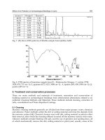
Heat loads, unlike temperature, are additive. Thus, it is possible to add the three profiles of Fig. 16
to obtain a combined heat-acceptance profile (Fig. 17). This is the FHCC and it shows total heating
needs in terms of the quantity of heat required and the temperature at which it is needed.
The exhaust profile of the proposed cogeneration plant is also shown in Fig. 17. In this case it
represents heat in the gas-turbine exhaust and is a straight line, neglecting the effect of condensation.
Note that the exhaust profile lies above the heat-acceptance curve, implying that heat can be trans-
ferred from the exhaust stream to the process. The vertical separation between the two profiles is a
measure of the available thermal driving force for heat transfer. Residual heat in the exhaust system,
after the process duties have been satisfied, overhangs the heat-acceptance curve (at the left-hand
end) and is lost up the stack.
Composite curves and profile matching provide a convenient way of representing the thermo-
dynamics of heat recovery in cogeneration systems. Implicit within the construction of Fig. 17 are
the requirements of the first law of thermodynamics, which demand a heat balance, and those of
the second law, which lead to a relationship between the temperatures at which heat is required
and the efficiency of the cogeneration system.
Analysis of the FHCC in Fig. 15 shows that all the needed process heat can be supplied by the
gas turbine exhaust. Hence, a further evaluation of the proposed cogeneration installation is justified.
2. Determine the annual fuel saving and payback period. Assemble the financial data in Table 11
from information available in plant records and estimates. These data show, for this proposed cogen-
eration installation, that the savings that can be obtained are: (a) boiler fuel savings, $4.1 million per
7.24 SECTION SEVEN
TABLE 11 Parameters Used to Evaluate Cogeneration Process
Displaced furnace fuel cost, $/million Btu 2
Furnace efficiency, % 85
Boiler fuel savings, $ million/yr 4.1
Displaced or exported power, $/kWh 0.045
Gas for cogeneration system, $/million Btu 3.50
Cogeneration gas cost, $ million/yr 12.2
Operating hours per year 8000
Power output, MW 36.3
Credit for cogenerated power, $ million/yr 13.1

Cogeneration efficiency, % 78.1
Installed cost, $ million 15.8
Total cash benefit, $ million/yr 5
Estimated payback, years 3
FIGURE 17 Total process heat-acceptance profile
is matched with prospective exhaust profile. (Power.)
Downloaded from Digital Engineering Library @ McGraw-Hill (www.digitalengineeringlibrary.com)
Copyright © 2004 The McGraw-Hill Companies. All rights reserved.
Any use is subject to the Terms of Use as given at the website.
ENVIRONMENTAL ENGINEERING
year; (b) credit for cogenerated power, $13.1 million per year; total savings = $4.1 million + $13.1
million = $17.2 million per year. The additional cost is that for the cogeneration gas which is burned
in the gas turbine, or $12.2 million. Thus, the net savings will be $17.2 million - $12.2 million = $5.0
million per year.
The payback time = installed cost, $/annual savings, $. Or, payback time = $15.8 million/$5.0 =
3.16, say 3.2 years. This is a relatively short payback time that would be acceptable in most industries.
Related Calculations Reciprocating internal-combustion engines are also often considered
where gas turbines appear to be a possible choice. The reason for this is that about 20 percent of
the heat content of fuel fired in a reciprocating engine is rejected in the exhaust gases and the
heat-rejection profile is similar to that of a gas turbine. And even more heat, about 30 percent, is
removed in cooling water at a temperature of 160°F (71°C) to 240°F (116°C). A further 5 per-
cent is available in the lubricating oil, usually below 180°F (82°C). The heat-rejection profile of
a reciprocating engine that closely matches the composite curve of the plant’s process is also
shown in Fig. 18.
A reciprocating engine has a higher overall efficiency than a gas turbine and therefore gener-
ates a greater cash benefit for the plant owner. For the scale of operation we are considering here,
it would be necessary to use several engines and the capital cost would be substantially greater
than that of a single gas turbine. As a result, payback periods for the two systems are about the
same.
Gas turbines are often mated with steam turbines in combined-cycle cogeneration plants. In its

basic form the combined-cycle power plant has the gas turbine exhausting into a heat-recovery
steam generator (HRSG) that supplies a steam-turbine cycle. This cycle is the most efficient
system for generating steam and/or electric power commercially available today. The cycle also
has significantly lower capital costs than competing nuclear and conventional fossil-fuel-fired
steam/electric stations. Other advantages of the combined-cycle plant are low air emissions, low
water consumption, reduced space requirements, and modular units which allow phased-in-
construction. And from an efficiency standpoint, even in a simple-cycle configuration, gas turbines
now exhibit efficiencies of between 30 and 35 percent, comparable to state-of-the-art fossil-
fuel-fired power stations.
Cogeneration, which is the simultaneous production of useful thermal energy and electric
power from a fuel source, or some variant thereof, is a good match for combined cycles. Expe-
rience with cogeneration and combined-cycle power plants has been most favorable. Figure 19
shows a variety of combined-cycle cogeneration plants using reheat in an HRSG to provide
ENVIRONMENTAL ENGINEERING 7.25
FIGURE 18 Exhaust-heat profile of reciprocating engine is
good fit with fired-heat composite curve of textile mill. (Power.)
Downloaded from Digital Engineering Library @ McGraw-Hill (www.digitalengineeringlibrary.com)
Copyright © 2004 The McGraw-Hill Companies. All rights reserved.
Any use is subject to the Terms of Use as given at the website.
ENVIRONMENTAL ENGINEERING
FIGURE 19 Combined-cycle gas-turbine cogeneration plants using reheat in an HRSG to provide steam for a steam-turbine generator. (Power.)
7.26
Downloaded from Digital Engineering Library @ McGraw-Hill (www.digitalengineeringlibrary.com)
Copyright © 2004 The McGraw-Hill Companies. All rights reserved.
Any use is subject to the Terms of Use as given at the website.
ENVIRONMENTAL ENGINEERING
steam for a steam-turbine generator. Flexibility is extended as gas turbines, steam turbines,
and HRSGs are added to a system. Reheat can improve thermal efficiency and performance
by several percentage points, depending on how it is integrated into the combined cycle.
Aeroderivative gas turbines, as part of a combined cycle, increasingly are finding application

in cogeneration in the under 100-MW capacity range. Cogeneration has the airline and defense
industries to thank for the rapid development of high-efficiency, long-running gas turbines at
extremely low research cost.
And the new large gas turbines have exhaust temperatures high enough to justify reheat
in the steam cycle without supplementary firing in a boiler. Depending on how the reheat
cycle is configured, thermal performance at rated conditions can vary by up to three per-
centage points.
The Public Utilities Regulatory Policies Act (PURPA) passed by Congress to help manage
energy includes incentives for efficient cogeneration systems. Cogeneration plants are
allowed to sell power to local electric utilities to increase the return on investment earned
from cogeneration.
A whole new energy-saving industry—termed nonutility generation (NUG)—has developed.
At this writing NUG plants in the 200- to 300-MW range are common. And the pipeline indus-
try which supplies natural-gas fuel for gas turbines is being restructured under the Federal Energy
Regulatory Commission (FERC). Lower fuel costs are almost certain to result.
While lower electricity and energy costs are in the offing, these must be balanced against
increased environmental requirements. The Clean Air Act Amendments of 1990 require better
cleaning of stack emissions to provide a cleaner atmosphere. Yet this same 1990 act allows utili-
ties to meet the required sulfur standard by installing suitable scrubber cleaning equipment, or by
switching to a low-sulfur fuel.
A utility may buy—from another utility which exceeds the required sulfur standard—
allowances to exhaust sulfur to the atmosphere. Each allowance permits a utility to emit 1 ton
(tonne) of sulfur to the atmosphere. Public auctions of these allowances are now being held peri-
odically by the Chicago Board of Trade.
Active discussions are underway at present over the suitability of selling sulfur allowances.
Some opponents to sulfur pollution allowances believe that their use will delay the cleanup that
ultimately must take place. Further, these opponents say, the pollution allowances delay the
installation of sulfur-removal equipment. Meanwhile, sulfuric acid rain (also called acid rain)
continues to plague communities in the path of a utility’s sulfur effluent.
Challenging the above view is the Environmental Defense Fund. Its view is that there are too

few allowances available to prevent the ultimate cleanup required by law.
The calculation data in this procedure are the work of A. P. Rossiter and S. H. Chang,
ICI/Tensa Services as reported in Power magazine, along with John Makansi, executive editor,
reporting in the same publication. Data on environmental laws are from the cited regulatory
agency or act.
GEOTHERMAL AND BIOMASS POWER-GENERATION ANALYSES
Compare the costs—installation and operating—of a 50-MW geothermal plant with that of a con-
ventional fossil-fuel-fired installation of the same rating. Likewise, compare plant availability for
each type. Brine available to the geothermal plant free-flows at 4.3 million lb/h (1.95 million kg/h)
at 450 lb/in
2
(gage) at 450°F (3100 kPa at 232°C).
Calculation Procedure
1. Estimate the cost of each type of plant. The cost of constructing a geothermal plant (i.e., an
electric-generating station that uses steam or brine from the ground produced by nature) is in the
ENVIRONMENTAL ENGINEERING 7.27
Downloaded from Digital Engineering Library @ McGraw-Hill (www.digitalengineeringlibrary.com)
Copyright © 2004 The McGraw-Hill Companies. All rights reserved.
Any use is subject to the Terms of Use as given at the website.
ENVIRONMENTAL ENGINEERING
$1500 to $2000 per installed kW range. This cost includes all associated equipment and the devel-
opment of the well field from which the steam or brine is obtained.
Using this cost range, the cost of a 50-MW geothermal station would be in the range of: 50 MW ×
($1500/kW) × 1000 = $75 million to 50 MW × ($2000/kW) × 1000 = $100 million. Fossil-fuel-fired
installations cost about the same—i.e., $1500 to $2000 per installed kW. Therefore, the two types of
plants will have approximately the same installed cost.
Department of Energy (DOE) estimates give the average cost of geothermal power at
5.7¢/kWh. This compares with the average cost of 2.4¢/kWh for fossil-fuel-based plants.
Advances in geothermal technology are expected to reduce the 5.7¢ cost significantly over the
next 40 years.

Because of the simplicity of geothermal plant design, maintenance requirements are relatively low.
Some modular plants even run unattended; and because maintenance is limited, plant availability is
high. In recent years geothermal-plant availability averaged 97 percent. Thus, the maintenance cost of
the usual geothermal plant is lower than a conventional fossil-fuel plant. Further, geothermal plants
can meet new emission regulations with little or no pollution-abatement equipment.
2. Choose the type of cycle to use. Tapping geothermal energy from liquid resources poses a
number of technical challenges—from drilling wells in a high-temperature environment to exces-
sive scaling and corrosion in plant equipment. But DOE-sponsored and private-sector R&D pro-
grams have effectively overcome most of these problems. Currently, there are more than
35 commercial plants exploiting liquid-dominated resources. Of the 800 MW of power generated
by these plants, 620 MW is produced by flash-type plants and 180 MW by binary-cycle units
(Fig. 20).
The flashed-steam plant is best suited for liquid-dominated resources above 350°F (177°C). For
lower-temperature sources, binary systems are usually more economical.
In flash-type plants, steam is produced by dropping the pressure of hot brine, causing it to “flash.”
The flashed steam is then expanded through a conventional steam turbine to produce power. In
binary-cycle plants, the hot brine is directed through a heat exchanger to vaporize a secondary fluid
which has a relatively low boiling point. This working fluid is then used to generate power in a
closed-loop Rankine-cycle system. Because they use lower-temperature brines than flash-type
plants, binary units (Fig. 20), are inherently more complex, less efficient, and have higher capital
equipment costs.
In both types of plants the spent brine is pumped down a well and reinjected into the resource
field. This is done for two reasons: (1) to dispose of the brine—which can be mineral-laden and
deemed hazardous by environmental regulatory authorities, and (2) to recharge the geothermal
resource.
One recent trend in the industry is to collect noncondensable gases (NCGs) purged from the con-
denser and reinject them along with the brine. Older plants use pollution-abatement devices to treat
NCGs, then release them to the atmosphere. Reinjection of NCGs with brine lowers operating costs
and reduces gaseous emissions to near zero.
Major improvements in flashed-steam plants over the past decade centered around: (1) improv-

ing efficiency through a dual-flash process and (2) developing improved water treatment processes
to control scaling caused by brines. The pressure of the liquid brine stream remaining after the first
flash is further reduced in a secondary chamber to generate more steam. This two-stage process can
generate 20 to 30 percent more power than single-flash systems.
Most of the recent improvements in binary-cycle plants have been made by applying new work-
ing fluids. The thermodynamic and transport properties of these fluids can improve cycle efficiency
and reduce the size and cost of heat-transfer equipment.
To illustrate: By using ammonia rather than the more common isobutane or isopentane, capital
cost can be reduced by 20 to 30 percent. It is also possible to improve the conversion efficiency by
using mixtures of working fluids, which in turn reduces the required brine flow rate for a given
power output.
A flashed-steam cycle will be tentatively chosen for this installation because the brine free-flows
at 450°F (232°C), which is higher than the cutoff temperature of 350°F (177°C) for binary systems.
7.28 SECTION SEVEN
Downloaded from Digital Engineering Library @ McGraw-Hill (www.digitalengineeringlibrary.com)
Copyright © 2004 The McGraw-Hill Companies. All rights reserved.
Any use is subject to the Terms of Use as given at the website.
ENVIRONMENTAL ENGINEERING
7.29
FIGURE 20 Energy from hot-water geothermal resources is converted by either a flash-type or binary-cycle plant. (Power.)
Downloaded from Digital Engineering Library @ McGraw-Hill (www.digitalengineeringlibrary.com)
Copyright © 2004 The McGraw-Hill Companies. All rights reserved.
Any use is subject to the Terms of Use as given at the website.
ENVIRONMENTAL ENGINEERING
7.30 SECTION SEVEN
FIGURE 21 Dual-flash process extracts up to 30 percent more power than older, single-flash units. (Power.)
An actual plant (Fig. 21), operating with these parameters uses two flashes. The first flash produces
623,000 lb/h (283,182 kg/h) of steam at 100 lb/in
2
(gage) (689 kPa). In the second flash an additional

262,000 lb/h (117,900 kg/h) of steam at 10 lb/in
2
(gage) (68.9 kPa) is produced.
Steam is cleaned in two trains of scrubbers, then expanded through a 54-MW, 3600-rpm, dual-
flow, dual-pressure, five-stage turbine-generator to produce 48.9 MW. Of this total, 47.5 MW is sold
to Southern California Edison Co. because of transmission losses.
The turbine exhausts into a surface condenser, coupled to a seven-cell cooling tower. About
40,000 lb/h (18,000 kg/h) of the high-pressure steam is required by the plant’s air ejectors to remove
NCGs from the main condenser at a rate of 6500 lb/h (2925 kg/h).
Because the liquid brine from the flash process is supersaturated, various solid compounds pre-
cipitate out of solution and must be removed to avoid scaling and fouling of the pumps, pipelines,
and injection wells. This is accomplished as the brine flows to the crystallizer and clarifier tanks
where, respectively, solid crystals grow and then are separated. The solids are dewatered and used in
construction-grade soil cement. The clarified brine is disposed of by pumping it into three injection
wells.
Related Calculations Geothermal generating plants are environmentally friendly because there
are no stack emissions from a boiler. Further, such plants do not consume fossil fuel, so they are
not depleting the world’s supply of such fuels. And by using the seemingly unlimited supply of
heat from the earth, such plants are contributing to an environmentally cleaner and safer world
while using a renewable fuel.
Another renewable fuel available naturally that is receiving—like geothermal power—greater
attention today is biomass. The most common biomass fuels used today are waste products and
residues left over from various industries, including farming, logging, pulp, paper, and lumber
production, and wood-products manufacturing. Wooden and fibrous materials separated from the
municipal waste stream also represent a major source of biomass.
Although biomass-fueled power plants currently account only for about 1 percent of the
installed generating capacity in the United States, or 8000 MW, they play an important role in
solving energy and environmental problems. Since the fuels burned in these facilities are consid-
ered waste in many cases, combustion yields the double benefits of reducing or eliminating dis-
posal costs for the seller and providing a low-emissions fuel source for the buyer. On a global

Downloaded from Digital Engineering Library @ McGraw-Hill (www.digitalengineeringlibrary.com)
Copyright © 2004 The McGraw-Hill Companies. All rights reserved.
Any use is subject to the Terms of Use as given at the website.
ENVIRONMENTAL ENGINEERING
scale, biomass firing could present even more advantages, such as: (1) there is no net buildup of
atmospheric CO
2
and air emissions are lower compared to many coal- or oil-fired plants. (2) Vast
areas of deforested or degraded lands in tropical and subtropical regions can be converted to prac-
tical use. Because much of the available land is in the developing regions of Latin America and
Africa, the fuels produced on these plantations could help improve a country’s balance of pay-
ments by reducing dependence on imported oil. (3) Industrialized nations could potentially phase
out agricultural subsidies by encouraging farmers to grow energy crops on idle land.
The current cost of growing, harvesting, transporting, and processing high-grade biomass
fuels is prohibitive in most areas. However, proponents are counting on the successful develop-
ment of advanced biomass-gasification technologies. They contend that biomass may be a more
desirable feedstock for gasification than coal because it is easier to gasify and has a very low
sulfur content, eliminating the need for expensive O
2
production and sulfur-removal processes.
One report indicates that integrated biomass-gasification–gas-turbine-based power systems
with efficiencies topping 40 percent should be commercially available soon. By 2025, efficien-
cies may reach 57 percent if advanced biomass-gasification–fuel-cell combinations become
viable. Proponents are optimistic because this technology is currently being developed for coal
gasification and can be readily transformed to biomass.
Data in this procedure are the work of M. D. Forsha and K. E. Nichols, Barber-Nichols Inc.,
for the geothermal portion, and Steven Collins, assistant editor, Power, for the biomass portion.
Data on both these topics were published in Power magazine.
ESTIMATING CAPITAL COST OF COGENERATION
HEAT-RECOVERY BOILERS

Use the Foster-Pegg* method to estimate the cost of the gas-turbine heat-recovery boiler system
shown in Fig. 22 based on these data: The boiler is sized for a Canadian Westinghouse 251 gas tur-
bine; the boiler is supplementary fired and has a single gas path; natural gas is the fuel for both the
gas turbine and the boiler; superheated steam generated in the boiler at 1200 lb/in
2
(gage) (8268 kPa)
and 950°F (510°C) is supplied to an adjacent chemical process facility; 230-lb/in
2
(gage) (1585-kPa)
saturated steam is generated for reducing NO
x
in the gas turbine; steam is also generated at 25 lb/in
2
(gage) (172 kPa) saturated for deaeration of boiler feedwater; a low-temperature economizer pre-
heats undeaerated feedwater obtained from the process plant before it enters the deaerator. Estimate
boiler costs for two gas-side pressure drops: 14.4 in (36.6 cm) and 10 in (25.4 cm), and without, and
with, a gas bypass stack. Table 12 gives other application data. Note: Since cogeneration will account
for a large portion of future power generation, this procedure is important from an environmental
standpoint. Many of the new cogeneration facilities planned today consist of gas turbines with heat-
recovery boilers, as does the plant analyzed in this procedure.
Calculation Procedure
1. Determine the average LMTD of the boiler. The average log mean temperature difference
(LMTD) of a boiler is indicative of the relative heat-transfer area, as developed by R. W. Foster-Pegg,
and reported in Chemical Engineering magazine. Thus, LMTD
avg
= Q
t
/C
t
, where Q

t
= total heat
exchange rate of the boiler, Btu/s (W); C
t
= conductance, Btu/s⋅F (W). Substituting, using data from
Table 12, LMTD
avg
= 81,837/1027 = 79.7°F (26.5°C).
2. Compute the gas pressure drop through the boiler. The gas pressure drop, ∆P inH
2
O (cmH
2
O) =
5C
t
/G, where G = gas flow rate, lb/s (kg/s). Substituting, ∆P = 5(1027/355.8) with a gas flow of
355.8 lb/s (161.5 kg/s), as given in Fig. 12; then ∆P = 14.4 inH
2
O (36.6 cmH
2
O). With a stack and
inlet pressure drop of 3 inH
2
O (7.6 cmH
2
O) and a supplementary-firing pressure drop of 3 inH
2
O
(7.6 cmH
2

O) given by the manufacturer, or determined from previous experience with similar
designs, the total pressure drop = 14.4 + 3.0 + 3.0 = 20.4 inH
2
O (51.8 cmH
2
O).
ENVIRONMENTAL ENGINEERING 7.31
Downloaded from Digital Engineering Library @ McGraw-Hill (www.digitalengineeringlibrary.com)
Copyright © 2004 The McGraw-Hill Companies. All rights reserved.
Any use is subject to the Terms of Use as given at the website.
ENVIRONMENTAL ENGINEERING
7.32
FIGURE 22 Gas-turbine and heat-recovery-boiler system. (Chemical Engineering.)
Downloaded from Digital Engineering Library @ McGraw-Hill (www.digitalengineeringlibrary.com)
Copyright © 2004 The McGraw-Hill Companies. All rights reserved.
Any use is subject to the Terms of Use as given at the website.
ENVIRONMENTAL ENGINEERING
3. Compute the system costs. The conductance cost component, Cost
ts
, is given by Cost
ts
, in thou-
sands of $, = 5.65[(C
sh
0.8
+ C
1
0.8
+ ⋅⋅⋅ + (C
n

0.8
) + 2(C
n
0.8
)], where C = conductance, Btu/s⋅F; (W), and
the subscripts represent the boiler elements listed in Table 12. Substituting, Cost
ts
, = 5.65(404.37) =
$2,285,000 in 1985 dollars. To update to present-day dollars, use the ratio of the 1985 Chemical
Engineering plant cost index (310) to the current year’s cost index thus: Current cost = (today’s plant
cost index/310)(cost computed above).
The steam-flow cost component, Cost
w
, in thousands of $ = 4.97(W
1
+ W
2
+ ⋅⋅⋅ + W
n
), where
Cost
w
= cost of feedwater, $; W = feedwater flowrate, lb/s (kg/s); the subscripts 1, 2, and n denote
different steam outputs. Substituting, Cost
w
= 4.97(59.14) = $294,000 in 1985 dollars, with a total
feedwater flow of 59.14 lb/s (26.9 kg/s).
The cost for gas flow includes connecting ducts, casing, stack, etc. It is proportional to the sum
of the separate gas flows, each raised to the power of 1.2. Or, cost of gas flow, Cost
g

, in thousands
of $ = 0.236(G
1
1.2
+ G
2
1.2
+ ⋅⋅⋅ + G
n
1.2
). Substituting, Cost
g
= 0.236(355.8)
1.2
= $272,000 with a gas
flow of 355.8 lb/s (161.5 kg/s) and no bypass stack.
The cost of a supplementary-firing system for the heat-recovery boiler in 1985 dollars is additional
to the boiler cost. Typical fuels for supplementary firing are natural gas or No. 2 fuel oil, or both. The
supplementary-firing system cost, Cost
f
, in thousands of $ = B/1390 + 30N + 20, where B = boiler
firing capacity in Btu (kJ) high heating value; N = number of fuels burned. For this installation with
one fuel, Cost
f
= 16,980/1390 + 30 + 20 = $62,000, rounded off. In this equation the 16,980 Btu/s
(17,914 kJ/s) is the high heating value of the fuel and N = 1 since only one fuel is used.
The total boiler cost (with base gas ∆P and no gas bypass stack) = total material cost + erection
cost, or $2,285,000 + 294,000 + 272,000 + 62,000 = $2,913,000 for the materials. A budget estimate
for the cost of erection = 25 percent of the total material cost, or 0.25 × $2,913,000 = $728,250. Thus,
the budget estimate for the erected cost = $2,913,000 + $728,250 = $3,641,250.

The estimated cost of the entire system—which includes the peripheral equipment, connections,
startup, engineering services, and related erection—can be approximated at 100 percent of the cost
of the major equipment delivered to the site, but not erected. Thus, the total cost of the boiler ready
for operation is approximately twice the cost of the major equipment material, or 2(boiler material
cost) = 2($2,913,000) = $5,826,000.
4. Determine the costs with the reduced pressure drop. The second part of this analysis reduces
the gas pressure drop through the boiler to 10 inH2O (25.4 cmH2O). This reduction will increase the
capital cost of the plant because much of the equipment will be larger.
Proceeding as earlier, the total pressure drop, ∆P = 10 + 3 + 3 = 16 inH
2
O (40.6 cmH
2
O). The
pressure drop for normal solidity (i.e., normal tube and fin spacing in the boiler) is ∆P
1
= 14.4 inH
2
O
ENVIRONMENTAL ENGINEERING 7.33
TABLE 12 Data for Heat Recovery Boiler*
LMTD, Q, C, C
0.8
°F Btu/s Btu/s⋅°F Btu/s⋅°F
Superheater 237 16,098 67.92 29.22
High evaporator 116 32,310 278.53 90.34
High economizer 40 11,583 290.3 93.39
Inter-evaporator 50.5 3,277 64.89 28.17
Inter-economizer 57 9,697 169.82 60.81
Deareator evaporator 46 6,130 134.43 50.44
Low economizer 131 2,742 20.93 11.39

Additional for superheater material 29.22
Additional for low-economizer material 11.39
Total 81,837 1,027 404.37
*See procedure for SI values in this table.
Source: Chemical Engineering.
Downloaded from Digital Engineering Library @ McGraw-Hill (www.digitalengineeringlibrary.com)
Copyright © 2004 The McGraw-Hill Companies. All rights reserved.
Any use is subject to the Terms of Use as given at the website.
ENVIRONMENTAL ENGINEERING
(36.6 cmH
2
O). For a different pressure drop, ∆P
2
, the surface cost, C
s
($), is at ∆P
2
, C
s
=
[1.67(∆P
1
/∆P
2
)
0.28
− 0.67](C
s
at P
1

). Substituting, C
s
= 1.67(14.4/10)
0.28
− 0.67 = 1.18 × base cost
from above. Hence, the surface cost for a pressure drop of 10 inH
2
O (25.4 cmH
2
O) = 1.18
($2,285,000) = $2,696,300.
The total material cost will then be $2,696,300 + $272,000 + $62,000, using the data from above,
or $3,324,300. Budget estimate for erection, as before = 1.25($3,324,300) = $4,155,375. And the
estimated system cost, ready to operate = 2($3,324,300) = $6,648,600.
Adding for a gas bypass stack, the gas-flow component is the same as before, $272,000. Then the
budget estimate of the installed cost of the gas bypass stack = 1.25($272,000) = $340,000. And the
total cost of the boiler ready for operation at a gas-pressure drop of 10 inH
2
O (25.4 cmH
2
O) with a
gas bypass stack = 2($3,324,300 + $272,000) = $7,192,600.
Related Calculations To convert the costs found in this procedure to current-day costs, assume
that the Chemical Engineering plant cost index today is 435, compared to the 1985 index of 310.
Then, today’s cost, $ = (today’s cost index/1985 cost index)(1985 plant or equipment cost, $).
Thus, for the first installation, today’s cost = (435/310)($5,826,000) = $8,175,194. And for the
second installation, today’s cost = (435/310)($7,192,600) = $10,092,842.
Boilers for recovering exhaust heat from gas turbines are very different from conventional
boilers, and their cost is determined by different parameters. Because engineers are becoming
more involved with cogeneration, the differences are important to them when making design and

cost estimates and decisions.
In a conventional boiler, combustion air is controlled at about 110 percent of the stoichiomet-
ric requirement, and combustion is completed at about 3000°F (1649°C). The maximum temper-
ature of the water (i.e., steam) is 1000°F (538°C), and the temperature difference between the gas
and water is about 2000°F (1093°C). The temperature drop of the gas to the stack is about 2500°F
(1371°C), and the gas/water ratio is consistent at about 1.1.
By contrast, the exhaust from a gas turbine is at a temperature of about 1000°F (538°C), and
the difference between the gas and water temperatures averages 100°F (56°C). The temperature
drop of the gas to the stack is a few hundred degrees, and the gas/water ratio ranges between 5
and 10. Because the airflow to a heat-recovery boiler is fixed by the gas turbine, the air varies
from 400 percent of the stoichiometric requirement of the fuel to the turbine (unfired boiler) to
200 percent if the boiler is supplementary fired.
In heat-recovery boilers, the tubes are finned on the outside to increase heat capture. Fins
in conventional boilers would cause excessive heat flux and overheating of the tubes.
Although the lower gas temperatures in heat-recovery boilers allow gas enclosures to be
uncooled internally insulated walls, the enclosures in conventional boilers are water-cooled
and refractory-lined.
Because the exhaust from a gas turbine is free of particles and contaminants, gas velocities past
tubes can be high, and fin and tube spacings can be close, without erosion or deposition. Because
the products of combustion in a conventional boiler may contain sticky residues, carbon, and ash
particles, tube spacing must be wider and gas velocities lower. Because of its configuration and
absence of refractories, the heat-recovery boiler used with gas turbines can be shop-fabricated to
a greater extent than conventional boilers.
These differences between conventional and heat-recovery boilers result in different cost rela-
tionships. With both operating on similar clean fuels, a heat-recovery boiler will cost more per
pound of steam and less per square foot (m
2
) of surface area than a conventional boiler. The cost
of a heat-recovery boiler can be estimated as the sum of three major parameters, plus other
optional parameters. Major parameters are: (1) the capacity to transfer heat (“conductance”), (2)

steam flow rate, and (3) gas flow rate. Optional parameters are related to the optional components
of supplementary firing and a gas bypass stack.
This procedure is the work of R. W. Foster-Pegg, Consultant, as reported in Chemical Engi-
neering magazine. Note that the costs computed by the given equations are in 1985 dollars.
Therefore, they must be updated to current costs using the Chemical Engineering plant cost
index.
7.34 SECTION SEVEN
Downloaded from Digital Engineering Library @ McGraw-Hill (www.digitalengineeringlibrary.com)
Copyright © 2004 The McGraw-Hill Companies. All rights reserved.
Any use is subject to the Terms of Use as given at the website.
ENVIRONMENTAL ENGINEERING
“CLEAN” ENERGY FROM SMALL-SCALE HYDRO SITES
A newly discovered hydro site provides a potential head of 65 ft (20 m). An output of 10,000 kW
(10 MW) is required to justify use of the site. Select suitable equipment for this installation based on
the available head and the required power output.
Calculation Procedure
1. Determine the type of hydraulic turbine suitable for this site. Enter Fig. 23 on the left at the
available head, 65 ft (20 m), and project to the right to intersect the vertical projection from the
required turbine output of 10,000 kW (10 MW). These two lines intersect in the standardized tubu-
lar unit region. Hence, such a hydroturbine will be tenatively chosen for this site.
2. Check the suitability of the chosen unit. Enter Table 13 at the top at the operating head range
of 65 ft (20 m) and project across to the left to find that a tubular-type hydraulic turbine with fixed
blades and adjustable gates will produce 0.25 to 15 MW of power at 55 to 150 percent of rated head.
These ranges are within the requirements of this installation. Hence, the type of unit indicated by
Fig. 23 is suitable for this hydro site.
Relation Calculations Passage of legislation requiring utilities to buy electric power from
qualified site developers is leading to strong growth of both site development and equipment
suitable for small-scale hydro plants. Environmental concerns over fossil-fuel-fired and nuclear
generating plants make hydro power more attractive. Hydro plants, in general, do not pollute the
air, do not take part in the acid-rain cycle, are usually remote from populated areas, and run for

up to 50 years with low maintenance and repair costs. Environmentalists rate hydro power as
“clean” energy available with little, or no, pollution of the environment.
To reduce capital cost, most site developers choose standard-design hydroturbines. With
essentially every high-head site developed, low-head sites become more attractive to developers.
Table 13 shows the typical performance characteristics of hydroturbines being used today. Where
there is a region of overlap in Table 13 or Fig. 23, site-specific parameters dictate choice and
whether to install large units or a greater number of small units.
Delivery time and ease of maintenance are other factors important in unit choice. Further,
the combination of power-generation and irrigation services in some installations make
ENVIRONMENTAL ENGINEERING 7.35
FIGURE 23 Traditional operating regimes of hydraulic turbines. New designs allow some
turbines to cross traditional boundaries. (Power.)
Downloaded from Digital Engineering Library @ McGraw-Hill (www.digitalengineeringlibrary.com)
Copyright © 2004 The McGraw-Hill Companies. All rights reserved.
Any use is subject to the Terms of Use as given at the website.
ENVIRONMENTAL ENGINEERING
hydroturbines more attractive from an environmental view because two objectives are obtained:
(1) “clean” power, and (2) crop watering.
Maintenance considerations are paramount with any selection; each day of downtime is lost
revenue for the plant owner. For example, bulb-type units for heads between 10 and 60 ft (3 and
18 m) have performance characteristics similar to those of Francis and tubular units, and are often
1 to 2 percent more efficient. Also, their compact and, in some cases, standard design makes for
smaller installations and reduced structural costs, but they suffer from poor accessibility. Some-
times the savings arising from the unit’s compactness are offset by increased costs for the water-
tight requirements. Any leakage can cause severe damage to the machine.
To reduce the costs of hydroturbines, suppliers are using off-the-shelf equipment. One way
this is done is to use centrifugal pumps operated in reverse and coupled to an induction motor.
Although this is not a novel concept, pump manufacturers have documented the capability of
many readily available commercial pumps to run as hydroturbines. The peak efficiency as a tur-
bine is at least equivalent to the peak efficiency as a pump. These units can generate up to 1 MW

of power. Pumps also benefit from a longer history of cost reductions in manufacturing, a wider
range of commercial designs, faster delivery, and easier servicing—all of which add up to more
rapid and inexpensive installations.
Though a reversed pump may begin generating power ahead of a turbine installation, it will
not generate electricity more efficiently. Pumps operated in reverse are nominally 5 to 10 percent
less efficient than a standard turbine for the same head and flow conditions. This is because
pumps operate at fixed flow and head conditions; otherwise efficiency falls off rapidly. Thus,
pumps do not follow the available water load as well unless multiple units are used.
With multiple units, the objective is to provide more than one operating point at sites with signifi-
cant flow variations. Then the units can be sequenced to provide the maximum power output for any
given flow rate. However, as the number of reverse pump units increases, equipment costs approach
those for a standard turbine. Further, the complexity of the site increases with the number of reverse
pump units, requiring more instrumentation and automation, especially if the site is isolated.
Energy-conversion-efficiency improvements are constantly being sought. In low-head appli-
cations, pumps may require specially designed draft tubes to minimize remaining energy after the
water exists from the runner blades. Other improvements being sought for pumps are: (1) modi-
fying the runner-blade profiles or using a turbine runner in a pump casing, (2) adding flow-control
devices such as wicket gates to a standard pump design or stay vanes to adjust turbine output.
Many components of hydroturbines are being improved to reduce space requirements and
civil costs, and to simplify design, operation, and maintenance. Cast parts used in older turbines
7.36 SECTION SEVEN
TABLE 13 Performance Characteristics of Common Hydroturbines
Operating head range Capacity range
% of % of design
Type Rated head, ft(m) rated head MW capacity
Vertical fixed-blade propeller 7–120 (3–54) and over 55–125 0.25–15 30–115
Vertical Kaplan (adjustable 7–66 (3–30) and over 45–150 1–15 10–115
blades and guide vanes)
Vertical Francis 25–300 (11–136) and over 50–150 and over 0.25–15 35–115
Horizontal Francis 25–500 (11–227) and over 50–125 0.25–10 35–115

Tubular (adjustable blades, 7–59 (3–27) 65–140 0.25–15 45–115
fixed gates)
Tubular (fixed blades, 7–120 (3–54) 55–150 0.25–15 35–115
adjustable gates)
Bulb 7–66 (3–30) 45–140 1–15 10–115
Rim generator 7–30 (3–14) 45–140 1–8 10–115
Right-angle-drive propeller 7–59 (3–27) 55–140 0.25–2 45–115
Cross flow 20–300 (9–136) and over 80–120 0.25–2 10–115
Source: Power.
Downloaded from Digital Engineering Library @ McGraw-Hill (www.digitalengineeringlibrary.com)
Copyright © 2004 The McGraw-Hill Companies. All rights reserved.
Any use is subject to the Terms of Use as given at the website.
ENVIRONMENTAL ENGINEERING
have largely been replaced by fabricated components. Stainless steel is commonly recommended
for guide vanes, runners, and draft-tube inlets because of better resistance to cavitation, erosion,
and corrosion. In special cases, there are economic tradeoffs between using carbon steel with a
suitable coating material and using stainless steel.
Some engineers are experimenting with plastics, but much more long-term experience is
needed before most designers will feel comfortable with plastics. Further, stainless steel material
costs are relatively low compared to labor costs. And stainless steel has proven most cost-effective
for hydroturbine applications.
While hydro power does provide pollution-free energy, it can be subject to the vagaries of the
weather and climatic conditions. Thus, at the time of this writing, some 30 hydroelectric stations
in the northwestern part of the United States had to cut their electrical output because the com-
bination of a severe drought and prolonged cold weather forced a reduction in water flow to the
stations. Purchase of replacement power—usually from fossil-fuel-fired plants—may be neces-
sary when such cutbacks occur. Thus, the choice of hydro power must be carefully considered
before a final decision is made.
This procedure is based on the work of Jason Makansi, associate editor, Power magazine, and
reported in that publication.

CENTRAL CHILLED-WATER SYSTEM DESIGN TO MEET
CHLOROFLUOROCARBON (CFC) ISSUES
Choose a suitable storage tank size and capacity for a thermally stratified water-storage system for a
large-capacity thermal-energy storage system for off-peak air conditioning for these conditions: Ther-
mal storage capacity required = 100,000 ton-h (35,169 kWh); difference between water inlet and outlet
temperatures = T = 20°F (36°C); allowable nominal soil bearing load in one location is 2500 lb/ft
2
(119.7 kPa); in another location 4000 lb/ft
2
(191.5 kPa). Compare tank size for the two locations.
Calculation Procedure
1. Compute the required tank capacity in gallons (liters) to serve this system. Use the relation C =
1800 S/∆T, where C = required tank capacity, gal; S = system capacity, ton-h; ∆T = difference between
inlet and outlet temperature, °F (°C). For this installation, C = 1800 (100,000)/20 = 9,000,000 gal
(34,065 m
3
).
2. Determine the tank height and diameter for the allowable soil bearing loads. Depending on
the proposed location of the storage tank, either the height or diameter may be a restricted dimen-
sion. Thus, tank height may be restricted by local zoning laws or possible interference with aircraft
landing or takeoff patterns. Tank diameter may be restricted by the ground area available. And the
allowable nominal soil bearing load will determine if the required amount of water can be stored in
one tank or if more than one tank will be required.
Starting with 2500-lb/ft
2
(119.7-kPa) bearing-load soil, assume a standard tank height of 40 ft
(12.2 m). Then the required tank volume will be V = 0.134C, where 0.134 = ft
3
/gal; or V = 0.134
(9,000,000) = 1,206,000 ft

3
(34,130 m
3
). The tank diameter is d = (4V/ph)
0.5
, where d = diameter in
feet (m). Or d = [4(1,206,000)/p40)]
0.5
= 195.93 ft; say 196 ft (59.7 m). This result is consistent with
the typical sizes, heights, and capacities used in actual practice, as shown in Table 14.
Checking the soil load, the area of the base of this tank is A = pd
2
/4 = p(196)
2
/4 = 30,172 ft
2
(2803 m
2
). The weight of the water in the tank is W = 8.35C = 75,150,000 lb (34,159 kg). This
will produce a soil bearing pressure of p = W/A lb/ft
2
(kPa). Or, p = 75,150,000/30,172 = 2491 lb/ft
2
(119.3 kPa). This bearing load is within the allowable nominal specified load of 2500 lb/ft
2
.
Where a larger soil bearing load is permitted, tank diameter can be reduced as the tank height is
increased. Thus, using a standard 64-ft (19.5-m) high tank with the same storage capacity, the
required diameter would be d = [4(1,206,000)/p64)]
0.5

= 154.9 ft (47.2 m). Soil bearing pressure will
then be W/A = 75,140,000/[p(154.9)
2
/4] = 3987.8 lb/ft
2
(190.9 kPa). This is within the allowable soil
bearing load of 4000 lb/ft
2
(191.5 kPa).
ENVIRONMENTAL ENGINEERING 7.37
Downloaded from Digital Engineering Library @ McGraw-Hill (www.digitalengineeringlibrary.com)
Copyright © 2004 The McGraw-Hill Companies. All rights reserved.
Any use is subject to the Terms of Use as given at the website.
ENVIRONMENTAL ENGINEERING
TABLE 14 Typical Thermal Storage Tank Sizes, Heights, Capacities*
Rated
thermal energy
Tank shell height (and nominal soil bearing load)
storage capacity, 64-ft shell height 40-ft shell height 24-ft shell height
ton-hours (4000 lb/ft
2
soil) (2500 lb/ft
2
) (1500 lb/ft
2
oil)
∆T, ∆T, ∆T, Gross volume, Tank diameter, Gross volume, Tank diameter, Gross volume, Tank diameter,
10°F15°F20°F gal ft gal ft gal ft
40,000 60,000 80,000 6,880,000 135 7,200,000 175 7,880,000 236
50,000 75,000 100,000 8,610,000 151 9,000,000 196 9,850,000 264

60,000 90,000 120,000 10,330,000 166 10,800,000 214 11,820,000 290
*See calculation procedures for SI values.
Source: Chicago Bridge & Iron Company.
7.38
Downloaded from Digital Engineering Library @ McGraw-Hill (www.digitalengineeringlibrary.com)
Copyright © 2004 The McGraw-Hill Companies. All rights reserved.
Any use is subject to the Terms of Use as given at the website.
ENVIRONMENTAL ENGINEERING
By reducing the storage capacity of the tank 4 percent to 8,610,000 gal (32,589 m
3
), the diame-
ter of the tank can be made 151 ft (46 m). This is a standard dimension for 64-ft (19-m) high tanks
with a 4000-lb/ft
2
(191.5-kPa) soil bearing load.
Related Calculations Thermal energy storage (TES) is environmentally desirable because it uses
heating, ventilating, and air-conditioning (HVAC) equipment and a storage tank to store heated or
cooled water during off-peak hours, allowing more efficient use of electric generating equipment.
The stored water is used to serve HVAC or industrial process loads during on-peak hours.
To keep investment, operating, and maintenance costs low, one storage tank can be used to store
both cool and warm water. Thermal stratification permits a smaller investment in the tank, piping, insu-
lation, and controls to produce a higher-efficiency system. Lower-density warm water is thermally
stratified from higher-density cool water without any mechanical separation in a full storage tank.
While systems using 200,000 gal (757 m
3
) of stored water are feasible, the usual minimum
size storage tank is 500,000 gal (1893 m
3
). Tanks as large as 4.4 million gal (16,654 m
3

) are cur-
rently in use in TES for HVAC and process needs. TES is also used for schools, colleges, facto-
ries, and a variety of other applications, where chlorofluorocarbon (CFC)-based refrigeration
systems must be replaced with less environmentally offensive refrigerants. TES systems can
easily be modified because the chiller (Fig. 24) is a simple piece of equipment.
ENVIRONMENTAL ENGINEERING 7.39
FIGURE 24 On-peak and off-peak storage discharging and recharging of thermally strat-
ified water-storage system. (Chicago Bridge & Iron Company.)
Downloaded from Digital Engineering Library @ McGraw-Hill (www.digitalengineeringlibrary.com)
Copyright © 2004 The McGraw-Hill Companies. All rights reserved.
Any use is subject to the Terms of Use as given at the website.
ENVIRONMENTAL ENGINEERING
As an added environmental advantage, the stored water in TES tanks can be used for fire pro-
tection. The full tank contents are continuously available as an emergency fire water reservoir.
With such a water reserve, the capital costs for fire-protection equipment can be reduced. Like-
wise, fire-insurance premiums may also be reduced. Where an existing fire-protection water tank
is available, it may be retrofitted for TES use.
Above-ground storage tanks (Fig. 25) are popular in TES systems. Such tanks are usually welded
steel, leak-free with a concrete ringwall foundation. Insulated to prevent heat gain or loss, such tanks
may have proprietary internal components for proper water distribution and stratification.
Some TES tanks may be installed partially, or fully, below grade. Before choosing partially
or fully below-grade storage, the following factors should be considered: (1) system
hydraulics may be complicated by a below-ground tank; (2) the tank must be designed for
external pressure, particularly when the tank is empty; (3) soil and groundwater conditions
may make the tank more costly; (4) local and national regulations for underground tanks may
increase costs; (5) the choice of water-treatment methods may be restricted for underground
tanks; (6) the total cost of an underground tank may be twice that of an above-ground tank.
The data and illustrations for this procedure were obtained from the Strata-Therm Thermal
Systems Group of the Chicago Bridge & Iron Company.
WORK REQUIRED TO CLEAN OIL-POLLUTED BEACHES

How much relative work is required to clean a 300-yd (274-m) long beach coated with heavy oil, if
the width of the beach is 40 yd (36.6 m), the depth of oil penetration is 20 in (50.8 cm), the beach
terrain is gravel and pebbles, the oil coverage is 60 percent of the beach, and the beach contains
heavy debris?
Calculation Procedure
1. Establish a work-measurement equation from a beach model. After the Exxon Valdez ran
aground on Bligh Reef in Prince William Sound, a study was made to develop a model and an equa-
tion that would give the relative amount of work needed to rid a beach of spilled oil. The relative
7.40 SECTION SEVEN
FIGURE 25 Typical chilled-water thermal-energy storage tank installation. (Chicago Bridge & Iron Company.)
Downloaded from Digital Engineering Library @ McGraw-Hill (www.digitalengineeringlibrary.com)
Copyright © 2004 The McGraw-Hill Companies. All rights reserved.
Any use is subject to the Terms of Use as given at the website.
ENVIRONMENTAL ENGINEERING
amount of work remaining, expressed in clydes, is defined as the amount of work required to clean
100 yd (91.4 m) of lightly polluted beach. As the actual cleanup progressed, the actual work required
was found to agree closely with the formula-predicted relative work indicated by the model and
equation that were developed.
The work-measurement equation, developed by on-the-scene Commander Peter C. Olsen, U.S.
Coast Guard Reserve, and Commander Wayne R. Hamilton, U.S. Coast Guard, is S =
(L/100)(EWPTCD), where S = standardized equivalent beach work units, expressed in clydes; L =
beach-segment length in yards or meters (considered equivalent because of the rough precision of
the model); E = degree of contamination of the beach expressed as: light oil = 1; moderate oil = 1.5;
heavy oil = 2; random tar balls and very light oil = 0.1; W = width of beach expressed as: less than
30 m = 1; 30 to 45 m = 1.5; more than 45 m = 2; P = depth of penetration of the oil expressed as:
less than 10 cm = 1; 10 to 20 cm = 2; more than 30 cm = 3; T = terrain of the beach expressed as:
boulders, cobbles, sand, mud, solid rock without vertical faces = 1; gravel/pebbles = 2; solid rock
faces = 0.1; C = percent of oil coverage of the beach expressed as: more than 67 percent coverage =
1; 50 to 67 percent = 0.8; less than 50 percent = 0.5; D = debris factor expressed as: heavy debris =
1.2; all others = 1.

2. Determine the relative work required. Using the given conditions, S = (300/100)(2 × 1.5 × 1 ×
1 × 0.8 × 1.2) = 8.64 clydes. This shows that the work required to clean this beach would be some
8.6 times that of cleaning 100 yd of lightly oiled beach. Knowing the required time input to clean
the “standard” beach (100 yd, lightly oiled), the approximate time to clean the beach being consid-
ered can be obtained by simple multiplication. Thus, if the cleaning time for the standard lightly
oiled beach is 50 h, the cleaning time for the beach considered here would be 50 (8.64) = 432 h.
Related Calculations The model presented here outlines—in general—the procedure to follow
to set up an equation for estimating the working time to clean any type of beach of oil pollution.
The geographic location of the beach will not in general be a factor in the model unless the beach
is in cold polar regions. In cold climates more time will be required to clean a beach because the
oil will congeal and be difficult to remove.
A beach cleanup in Prince William Sound was defined as eliminating all gross amounts of oil,
all migratory oil, and all oil-contaminated debris. This definition is valid for any other polluted
beach be it in Europe, the Far East, the United States, etc.
Floating oil in the marine environment can be skimmed, boomed, absorbed, or otherwise
removed. But oil on a beach must either be released by (1) scrubbing or (2) steaming and floated
to the nearby water where it can be recovered using surface techniques mentioned above.
Where light oil—gasoline, naphtha, kerosene, etc.—is spilled in an accident on the water, it
will usually evaporate with little damage to the environment. But heavy oil—No. 6, Bunker C,
unrefined products, etc.—will often congeal and stick to rocks, cobbles, structures, and sand.
Washing such oil products off a beach requires the use of steam and hot high-pressure water.
Once the oil is freed from the surfaces to which it is adhering, it must be quickly washed away
with seawater so that it flows to the nearby water where it can be recovered. Several washings
may be required to thoroughly cleanse a badly polluted beach.
The most difficult beaches to clean are those comprised of gravel, pebbles, or small boulders.
Two reasons for this are: (1) the surface areas to which the oil can adhere are much greater, and
(2) extensive washing of these surface areas is required. This washing action can carry away the
sand and the underlying earth, destroying the beach. When setting up an equation for such a
beach, this characteristic should be kept in mind.
Beaches with larger boulders having a moderate slope toward the water are easiest to clean.

Next in ease of cleaning are sand and mud beaches because thick oil does not penetrate deeply in
most instances.
Use this equation as is, and check its results against actual cleanup times. Then alter the equa-
tion to suit the actual conditions and personnel met in the cleanup.
The model and equation described here are the work of Commander Peter C. Olsen, U.S.
Coast Guard Reserve, and Commander Wayne R. Hamilton, U.S. Coast Guard, as reported in
government publications.
ENVIRONMENTAL ENGINEERING 7.41
Downloaded from Digital Engineering Library @ McGraw-Hill (www.digitalengineeringlibrary.com)
Copyright © 2004 The McGraw-Hill Companies. All rights reserved.
Any use is subject to the Terms of Use as given at the website.
ENVIRONMENTAL ENGINEERING
SIZING EXPLOSION VENTS FOR INDUSTRIAL STRUCTURES
Choose the size of explosion vents to relieve safely the maximum allowable overpressure of 0.75 lb/in
2
(5.2 kPa) in the building shown in Fig. 26 for an ethane/air explosion. Specify how the vents will be
distributed in the structure.
Calculation Procedure
1. Determine the total internal surface area of Part A of the building. Using normal length and
width area formulas for Part A, we have: Building floor area = 100 × 25 = 2500 ft
2
(232.3 m
2
); front
wall area = 12 × 100 = 1200 ft
2
– 12 × 20 = 960 ft
2
(89.2 m
2

); rear wall area = 12 × 100 = 1200 ft
2
(111.5 m
2
); end wall area = 2 × 25 × 12 + 2 × 25 × 3/2 = 675 ft
2
(62.7 m
2
); roof area = 2 × 3 × 100 =
600 ft
2
(55.7 m
2
). Thus, the total internal surface area of Part A of the building is 2500 + 960 + 1220 +
600 = 5935 ft
2
(551.4 m
2
).
7.42 SECTION SEVEN
FIGURE 26 Typical industrial building for which explosion vents are sized.
Downloaded from Digital Engineering Library @ McGraw-Hill (www.digitalengineeringlibrary.com)
Copyright © 2004 The McGraw-Hill Companies. All rights reserved.
Any use is subject to the Terms of Use as given at the website.
ENVIRONMENTAL ENGINEERING
2. Determine the total internal surface area of Part B of the building. Using area formulas, as
before: Floor area = 50 × 20 = 1000 ft
2
(92.9 m
2

): side wall area = 2 × 50 × 12 = 1200 ft
2
(111.5 m
2
)
front wall area = 20 × 12 = 240 ft
2
(22.3 m
2
); roof area = 50 × 20 = 1000 ft
2
(92.9 m
2
); total internal
surface area of Part B is 1000 + 1200 + 240 + 1000 = 3440 ft
2
(319.6 m
2
).
3. Compute the vent area required. Using the relation A
v
= CA
s
/(P
red
)
0.5
, where A
v
= required vent

area, m
2
; C = deflagration characteristic of the material in the building, (kPa)
0.5
, from Table 15; A
s
=
internal surface area of the structure to be protected, m
2
. For this industrial structure, A
v
= 0147
(551.4 + 319.6)/(5.17)
0.5
= 180.1 m
2
(1939 ft
2
) total vent area.
The required vent area should be divided proportionately between Part A and Part B of the build-
ing, or Part A vent area = 180.1(551.4/871.0) = 114 m
2
(1227 ft
2
); Part B vent area = 180.1(319.6/
871.0) = 66.1 m
2
(712 ft
2
).

The required vent area should be distributed equally over the external wall and roof areas in each
portion of the building. Before final choice of the vent areas to be used, the designer should consult
local and national fire codes. Such codes may require different vent areas, depending on a variety of
factors such as structure location, allowable overpressure, and gas mixture.
Related Calculations This procedure is the work of Tom Swift, a consultant, reported in
Chemical Engineering. In his explanation of his procedure he points out that the word explosion
is an imprecise term. The method outlined above is intended for those explosions known as
deflagrations—exothermic reactions that propagate from burning gases to unreacted materials by
conduction, convection, and radiation. The great majority of structural explosions at chemical
plants are deflagrations.
The equation used in this procedure is especially applicable to “low-strength” structures
widely used to house chemical processes and other manufacturing operations. This equation is
useful for both gas and dust deflagrations. It applies to the entire subsonic venting range. Nomen-
clature for Table 15 is given as follows:
A
s
Internal surface area of structure to be protected, m
2
A
v
Vent area, m
2
B Dimensionless constant
C Deflagration characteristic, (kPa)
1/2
ENVIRONMENTAL ENGINEERING 7.43
TABLE 15 Parameters for Vent Area Equation*
S
u
r

u
P
max
Material G¢ P
0
Methane 1.1 × 10
–3
8.33
Ethane 1.2 × 10
–3
9.36
Propane 1.2 × 10
–3
9.50
Pentane 1.3 × 10
–3
9.42
Ethylene 1.9 × 10
–3
9.39
Material C, (kPa)
1/2
Methane 0.41
Ethane 0.47
Propane 0.48
Pentane 0.51
Ethylene 0.75
ST 1 dusts 0.26
ST 2 dusts 0.30
Downloaded from Digital Engineering Library @ McGraw-Hill (www.digitalengineeringlibrary.com)

Copyright © 2004 The McGraw-Hill Companies. All rights reserved.
Any use is subject to the Terms of Use as given at the website.
ENVIRONMENTAL ENGINEERING
C
D
Discharge coefficient
G¢ Maximum subsonic mass flux through vent, kg/m
2
⋅s
P
f
Overpressure, kPa
P
max
Maximum deflagration pressure in a sealed spherical vessel, kPa
P
O
Initial (ambient) pressure, kPa
P
red
Maximum reduced explosion pressure that a structure can withstand, kPa
S
u
Laminar burning velocity, m/s
g
b
Ratio of specific heats of the combustion gases
r
u
Density of the unburnt gases, kg/m

3
l Turbulence enhancement factor
With increased interest in the environment by regulatory authorities, greater attention is being
paid to proper control and management of industrial overpressures. Explosion vents that are prop-
erly sized will protect both the occupants of the building and surrounding structures. Therefore,
careful choice of explosion vents is a prime requirement of sensible environmental protection.
INDUSTRIAL BUILDING VENTILATION
FOR ENVIRONMENTAL SAFETY
Determine the ventilation requirements to maintain interior environmental safety of a pump and com-
pressor room in an oil refinery in a cool-temperate climate. Floor area of the pump and compressor
room is 2000 ft
2
(185.8 m
2
) and room height is 15 ft (4.6 m); gross volume = 30,000 ft
3
(849 m
3
). The
room houses two pumps—one of 150 hp (111.8 kW) with a pumping temperature of 350°F (177°C),
and one of 75 hp (55.9 kW) with a pumping temperature of 150°F (66°C). Also housed in the room
is a 1000-hp (745.6-kW) compressor and a 50-hp (37.3-kW) compressor.
Calculation Procedure
1. Determine the hp-deg for the pumps. The hp-deg = pump horsepower × pumping temperature.
For these pumps, the total hp-deg = (150 × 350) + (75 × 150) = 63,750 hp-deg (19,789 kW-deg).
Enter Fig. 27 on the left axis at 63,750 and project to the diagonal line representing the ventilation
requirements for pump rooms in cool-temperate climates. Then extend a line vertically downward to
the bottom axis to read the air requirement as 7200 ft
3
/min (203.8 m

3
/min).
The compressors require a total of 1050 hp (782.9 kW). Enter Fig. 27 on the right-hand axis at
1050 and project horizontally to cool-temperate climates for compressor and machinery rooms. From
the intersection with this diagonal project vertically to the top axis to read 2200 ft
3
/min (62.3 m
3
/min)
as the ventilation requirement.
Since the ventilation requirements of pumps and compressors are additive, the total ventilation-
air requirement for this room is 7200 + 2200 = 9400 ft
3
/min (266 m
3
/min).
2. Check to see if the computed ventilation flow meets the air-change requirements. Use the
relation N = 60 F/V, where N = number of air changes per hour; F = ventilating-air flow rate, ft
3
/min
(m
3
/min); V = room volume, ft
3
(m
3
). Using the data for this room, N = 60(9400)/30,000 = 18.8 air
changes per hour.
Figure 27 is based on a minimum of 10 air changes per hour for summer and 5 air changes per
hour for winter. Since the 18.8 air changes per hour computed exceeds the minimum of 10 changes

per hour on which the chart is based, the computed air flow is acceptable.
7.44 SECTION SEVEN
Downloaded from Digital Engineering Library @ McGraw-Hill (www.digitalengineeringlibrary.com)
Copyright © 2004 The McGraw-Hill Companies. All rights reserved.
Any use is subject to the Terms of Use as given at the website.
ENVIRONMENTAL ENGINEERING
In preparing the chart in Fig. 27 the climate lines are based on ASHRAE degree-day listings,
namely: Cool, temperate climates, 5000 degree-days and up; average climates, 2000 to 5000 degree-
days; warm climates, 2000 degree-days maximum.
3. Select the total exhaust-fan capacity. An exhaust fan or fans must remove the minimum com-
puted ventilation flow, or 9400 ft
3
/min (266 m
3
/min) for this room. To allow for possible errors in
room size, machinery rating, or temperature, choose an exhaust fan 10 percent larger than the com-
puted ventilation flow. For this room the exhaust fan would therefore have a capacity of 1.1 × 9400 =
10,340 ft
3
/min (292.6 m
3
/min). A fan rated at 10,500 or 11,000 ft
3
/min (297.2 or 311.3 m
3
/min),
depending on the ratings available from the supplier, would be chosen.
Related Calculations Ventilation is environmentally important and must accomplish two goals:
(1) Removal of excess heat generated by machinery or derived from hot piping and other objects;
(2) removal of objectionable, toxic, or flammable gases from process pumps, compressors, and

piping.
The usual specifications for achieving these goals commonly call for an arbitrary number of
hourly air changes for a building or room. However, these specifications vary widely in the
ENVIRONMENTAL ENGINEERING 7.45
FIGURE 27 Chart for determining building ventilation requirements. (Chemical Engineering.)
Downloaded from Digital Engineering Library @ McGraw-Hill (www.digitalengineeringlibrary.com)
Copyright © 2004 The McGraw-Hill Companies. All rights reserved.
Any use is subject to the Terms of Use as given at the website.
ENVIRONMENTAL ENGINEERING
number of air changes required, and use inconsistent design methods for ventilation. The method
given in this procedure will achieve proper results, based on actual applications.
Because of health and explosion hazards, workers exposed to toxic or hazardous vapors and
gases should be protected against dangerous levels [threshold limit values (TLV)] and explosion
hazards [lower explosive limit (LEL)] by diluting workspace air with outside air at adequate ven-
tilation rates. If a workspace is protected by adequate ventilation rates for health (i.e., below TLV)
purposes, the explosion hazard (LEL) will not exist. The reason for this is that the health air
changes far exceed those required for explosion prevention.
To render a workspace safe in terms of TLV, the number of ft
3
/min (m
3
/min) of dilution air,
A
d
, required can be found from: A
d
= [1540 × S × T/(M × TLV)]K, or in SI, A
dm
= m
3

/min =
0.0283A
d
, where S = gas or vapor expelled over an 8-h period, lb (kg); M = molecular weight
of vapor or gas; TLV = threshold limit value, ppm; T = room temperature, absolute °R(K);
K = air-mixing factor for nonideal conditions, which can vary from 3 to 10, depending on
actual space conditions and the efficiency of the ventilation-air distribution system.
If the space temperature is assumed to be 100°F (37.8°C) (good average summer conditions),
the above equation becomes A
d
= [862,400 × S/(M × TLV)]K.
For every pound (kg) of gas or vapor expelled of an 8-h period, when S = 1, the second equa-
tion becomes A
d
= [862,400/(M × TLV)]K. For values of S less or greater than unity, simple mul-
tiplication can be used.
It is only for ideal mixing that K = 1. Hence, K must be adjusted upward, depending on ven-
tilation efficiency, operation, and the particular system application.
If mixing is perfect and continuous, then each air change reduces the contaminant concentra-
tion to about 35 percent of that before the air change. Perfect mixing is seldom attainable, how-
ever, so a room mixing factor, K, ranging from 3 to 10 is recommended in actual practice.
The practical mixing factor for a particular workspace is at best an estimate. Therefore, some
flexibility should be built into the ventilation system in anticipation of actual operations. For
small enclosures, such as ovens and fumigation booths, K-values range from 3 to 5. If you are not
familiar with efficient mixing within enclosures, use a K-factor equal to 10. Then your results will
be on the safe side. Figure 27 is based on a K-value equal to 8 to 10. Table 16 gives K-factors for
ventilation-air distribution systems as indicated.
In some installations, heat generated by rotating equipment (pumps, compressors, blowers)
process piping, and other equipment can be calculated, and the outside-air requirements for dilu-
tion ventilation determined. In most cases, however, the calculation is either too cumbersome and

time consuming or impossible.
Figure 27 was developed from actual practice in the chemical-plant and oil-refinery busi-
nesses. The chart is based on a closed processing system. Hence, air quantities found from the
chart are not recommended if (1) the system is not closed or (2) if abnormal operating conditions
prevail that permit the escape of excessive amounts of toxic and explosive materials into the
workplace atmosphere.
For these situations, special ventilation measures, such as local exhaust through hoods, are
required. Vent the exhaust to pollution-control equipment or, where permitted, directly outdoors.
Figure 27 and the procedure for determining dilution-air ventilation requirements were devel-
oped from actual tests of workspace atmospheres within processing buildings. Design and oper-
ating show that by supplying outside air into a building near the floor, and exhausting it high
7.46 SECTION SEVEN
TABLE 16 K-values for Various Ventilation-Air Distribution Systems*
K-values Distribution system
1.2–1.5 Perforated ceiling
1.5–2.0 Air diffusers
2.0–3.0 Duct headers along ceiling with branch headers pointing downward
3.0 and up Window fans, wall fans, and the like
*Chemical Engineering.
Downloaded from Digital Engineering Library @ McGraw-Hill (www.digitalengineeringlibrary.com)
Copyright © 2004 The McGraw-Hill Companies. All rights reserved.
Any use is subject to the Terms of Use as given at the website.
ENVIRONMENTAL ENGINEERING
(through the roof or upper outside walls), safe and comfortable conditions can be attained. Use
of chevron-type stormproof louvers permits outside air to enter low in the room.
The chevron feature causes the air to sweep the floor, picking up heat and diluting gases and
vapors on the way up to the exhaust fan, (Fig. 28).
In the system shown in Fig. 28 there are a number of features worth noting. With low-level
distribution and adequate high exhaust, only the internal plant heat load (piping, equipment) is of
importance in maintaining desirable workspace conditions. Wall and transmission heat loads are

swept out of the building and do not reach the work areas. Even the temperature rise caused by
the plant load occurs above the work level. Hence, low-level distribution of the supply air main-
tains the work area close to supply-air temperatures.
For any installation, it is good practice to check the ratio of hp-deg/ft
2
(kW-deg/m
2
) of floor
area. When this ratio exceeds 100, consider installing a totally enclosed ventilation system for
cooling. This should be complete with ventilating fans taking outside air, preferably from a high
stack, and discharging through ductwork into a sheetmetal motor housing.
The result is a greater use of outside air for cooling through a confined system at a lower ven-
tilation rate. Ventilation air flow needs may be obtained from the equipment manufacturer or
directly from the chart (Fig. 27). The remainder of the building may be ventilated as usual, based
either on the absence of equipment or on any equipment outside the ventilation enclosure.When
designing the duct system, take care to prevent moisture entrainment with the incoming
airstream.
This procedure is the work of John A. Constance, P.E., consultant, as reported in Chemical
Engineering.
ESTIMATING POWER-PLANT THERMAL POLLUTION
A steam power plant has a 1000-MW output rating. Find the cooling-water thermal pollution by this
power plant when using a once-through cooling system for the condensers if the plant thermal effi-
ciency is 30 percent.
ENVIRONMENTAL ENGINEERING 7.47
FIGURE 28 Ventilation system for effective removal of plant heat
loads. (Chemical Engineering.)
Downloaded from Digital Engineering Library @ McGraw-Hill (www.digitalengineeringlibrary.com)
Copyright © 2004 The McGraw-Hill Companies. All rights reserved.
Any use is subject to the Terms of Use as given at the website.
ENVIRONMENTAL ENGINEERING

Calculation Procedure
1. Determine the amount of heat added during plant operation. The general equation for power-
plant efficiency is E = W/Q
A
, where E = plant net thermal efficiency, %; W = plant net output, MW;
Q
A
= heat added, MW. For this plant, Q
A
= W/E = 1000/0.30 = 3333 MW.
2. Compute the heat rejected by this plant. The general equation for heat rejected is Q
R
= (W/E − W),
Q
R
= heat rejected, MW. For this power plant, Q
R
= (1000/0.3 − 1000) = 2333 MW. Thus, this plant
will reject 2333 MW to the condenser cooling water.
The heat rejected to the cooling water will be absorbed by the river, lake, or ocean providing the
water pumped through the condenser. Depending on the thermal efficiency of the plant, the required
cooling-water flow for the condenser will range from 250 × 10
6
lb/h, or 65,000 ft
3
/min (30 m
3
/s) to
400 × 10
6

lb/h or 100,000 ft
3
/min (50 m
3
/s). The discharged water in a once-through cooling system
will be 20 to 25°F (11 to 14°C) higher in temperature than the entering water.
3. Assess the effects of this thermal pollution. Warm water discharged in large volume to a
restricted water mass may affect the ecosystem in a deleterious way. Fish and plant life, larvae,
plankton, and other organisms can be damaged or have a high mortality rate. If chlorine is used to
control condenser scaling, the effect on the ecosystem can be more damaging.
If the warm condenser cooling water is discharged into a large body of water, such as a major
river or ocean, the effect on the ecosystem can be more beneficial than deleterious. Thus, well-
planned cooling-water outlets can be used to increase fish production in hatcheries. In agriculture,
the warm-water discharge can be used to markedly increase the output of greenhouses and open
fields in cold climates. Thus, the overall effect of thermal pollution can be positive, if the pollution
energy is used in an antipolluting manner.
Related Calculations Since thermal and atmospheric pollution are associated with the genera-
tion of electricity, environmental engineers are seeking ways to reduce electricity use. Personal
computers (PCs) are big users of electricity today. At the time of this writing, PCs consume some
5 percent of commercial energy used in the United States.
Typical PCs use 150 to 200 W of power when in use, or just on but not in use. Some 30 to
40 percent of PCs are left on overnight and during weekends. The extra electricity which must
be generated to carry this PC load leads to more thermal and air pollution.
New PCs have “sleep” circuitry which reduces the electrical load to 30 W when the computer
is not being used. Such microprocessors will reduce the electrical load caused by PCs. This, in
turn, will reduce thermal and air pollution produced by power-generating plants.
Internal-combustion engines—diesel, gas, and gas turbines—produce both thermal and air
pollution. To curb this pollution and wrest more work from the fuel burned, cogeneration is being
widely applied. Heat is extracted from the internal-combustion engine’s cooling water for use in
process or space heating. In addition, exhaust gases are directed through heat exchangers to

extract more heat from the internal-combustion engine exhaust. Thus, environmental considera-
tions are met while conserving fuel. This is one reason why cogeneration is so popular today.
Compute the heat recovery from cogeneration using the many concepts given earlier in this
section. Try to combine both heat recovery and pollution reduction; then the required investment
will be easier to justify from an economic standpoint.
7.48 SECTION SEVEN
Downloaded from Digital Engineering Library @ McGraw-Hill (www.digitalengineeringlibrary.com)
Copyright © 2004 The McGraw-Hill Companies. All rights reserved.
Any use is subject to the Terms of Use as given at the website.
ENVIRONMENTAL ENGINEERING