UNSTEADY AERODYNAMICS, AEROACOUSTICS AND AEROELASTICITY OF TURBOMACHINES Episode 10 ppt
Bạn đang xem bản rút gọn của tài liệu. Xem và tải ngay bản đầy đủ của tài liệu tại đây (1.57 MB, 50 trang )
464
Introduction
Transonic flows about streamlined bodies are strongly affected, particularly
near the shock location, by unsteady excitations. Experimental and computa-
tional studies [1, 2] have shown that the unsteady pressure distribution along
the surface of an airfoil or a cascade blade in unsteady transonic flow exhibits
a significant bulge near the shock location. Tijdeman and Seebass [3] reported
that the unsteady pressure bulge and its phase variation resulted from non-
linear interaction between the mean and unsteady flows. This non-linear in-
teraction causes a shift in the shock location, which produces the observed
large bulge in the unsteady pressure distribution. Studies [4] on choked flutter
have shown that, in unsteady transonic flows around a single airfoil, the shock
motion, and thus the pressure distribution along the surface, can be critical re-
garding to the self-exciting oscillations of the airfoil. It was also shown that
the mean flow gradients are of high importance regarding the time response
of the unsteady pressure distribution on the airfoil surface. Beside, numeri-
cal computations [5] pointed out that the exact location of the transition point
could strongly affect the prediction of stall flutter. Further studies [6] sug-
gested that this sharp rise in the unsteady pressure distribution was due to the
near sonic condition, and that the near-sonic velocity acts as a barrier they
identified as acoustic blockage preventing acoustic disturbances from propa-
gating upstream in a similar way to the shock in transonic flows. A transonic
convergent-divergent nozzle experimentally investigated by Ott et al [7] was
thereafter used as a model to investigate the non-linear acoustic blockage. An-
alytical and numerical computations [8, 9, 10, 11] were then carried out to
analyze and quantify the upstream and downstream propagation of acoustic
disturbances in the nozzle.
Similarly, in order to focus the present analysis on essential features, the
investigation has been carried out in a simple geometry such as a 2D conver-
gent divergent nozzle. Special influences of leading and trailing edges, and
interblade row region interactions are therefore avoided.
1. Experimental model
1.1 Test facility
The test section was designed highly modular to be able to insert differ-
ent test objects, so called ’bumps’, in a 100x120mm rectangular channel as
sketched in figure 1(a). A continuous air supply is provided by a screw com-
pressor driven by a 1MW electrical motor and capable of reaching a maximum
mass flow up to 4.7 kg/s at 4 bar. A cooling system allows a temperature range
from 30
o
Cto180
o
C. The adjustment of different valves also allows the exper-
Study of Nonlinear Interactions in Two-Dimensional Transonic Nozzle Flow 465
imentalist to control independently the mass flow and the pressure level in the
test section in the respective range of M
i
=0.1 − 0.8 and Re =
ρ
air
U
∞
d
ν
air
=
1.87 10
4
-1.5710
6
with d =0.26m, ρ
air
=0.54-4.48 kg/m
3
and ν
air
=1.5
10
−5
m
2
/s.
(a) Modular test section (b) Traverse mechanism for 2D bump
Figure 1. Transonic wind tunnel test section facility
1.2 Test object and instrumentation
The investigated test object consists of a long 2D bump, presented in figure
1(b), which can slide through the width of the test section using the traverse
mechanism and inflated O-ring sealing system . The nozzle geometry thus
consists of a 100mm wide and 120mm high flat channel with a 10.48mm max-
imum thickness and 184mm long 2D bump on the lower wall. The beginning
of the curvatures was chosen as the origin of the X-axis (x=0mm). The Y-axis
and Z-axis were set to be aligned with the channels’s width and height respec-
tively to form an orthogonal basis. The profile coordinates of the bump are
presented in table A.1.
The bump is equipped with one row of 100 hot film sensors, and three stag-
gered rows of 52 pressure taps each. The traverse mechanism fixed on the side
window allows the displacement of both the pressure tap rows and the hot film
sensors through the width of the channel. As a result, by sliding the 2D bump
and successively position each rows of pressure taps at the same location in the
channel will provide a spatial resolution measurements of 1.5mm for pressure
measurements. Unsteady pressure measurements were performed using fast
response Kulite transducers glued in protective pipes. Each pipe was designed
with a locking device so that it could be inserted in any of the already instru-
mented pressure hole located underneath the sliding 2D bump.
466
1.3 Unsteady perturbation generator
With the aim at simulating potential interaction in turbomachines, the "quasi
steady" shock wave was put into oscillations using a rotating elliptical cam
placed at x=625mm in the reference system of the bump. A DC motor was
used to rotate the cam up to 15,000RPMs in order to generate pressure per-
turbations up to 500Hz. The rotating speed was monitored using an optical
encoder located directly on the shaft of the motor. Rotating speed fluctuations
and time drift were measured under ±0.024% in the worst case. Furthermore,
a TTL pulse generated by the motor was used as a reference signal during
unsteady pressure measurements and Schlieren visualizations in order to cor-
relate both measuring techniques.
1.4 Measuring techniques
Steady state pressure measurements were performed using a 208-channels
’low speed’ data acquisition system. The scanners used feature a pressure
range of ±100kPa relative to atmosphere with an accuracy of ±0.042% full
scale. Taking into account the digital barometer, the overall accuracy for steady
state pressure measurements is about ±43.5Pa. The sampling frequency and
sampling time were respectively set to 10Hz and 200s in order to ’capture’ the
lowest frequencies.
Additionally, a 32-channels high frequency data acquisition and storage sys-
tem was used for unsteady pressure measurements. Accounting for the res-
onance frequency of the capillarity pipes between the bump surface and the
transducer, the sampling frequency was set to 8kHz with a low pass filter at
4kHz to avoid bias effects. Each channel was connected to a fast response
Kulite transducer and individually programmed to fully use the 16bit AD con-
version. A static calibration of all fast response transducers was performed
prior and after the measurements in order to reduce the systematic error related
to the drift of the sensitivity and offset coefficients. Furthermore, a dynamic
calibration was performed on all pressure taps in order to estimate the damp-
ing and time delay of propagating pressure waves through the capillarity tubes.
The unsteady pressure measurements were thereafter corrected to account for
the above estimated damping and phase-lag.
Finally, a conventional Schlieren system connected to a high speed CCD
camera was used to monitor the shock motion throughout the whole test section
height up to 8kHz. A special feature of the camera allows the display of the
TTL signal position directly onto the pictures for referencing purpose during
later post treatment. The sampling frequency and shutter speed of the camera
were optimally set up depending on the perturbation frequency in order to ob-
tain approximately 20 pictures per unsteady cycle (up to 500Hz). The spatial
Study of Nonlinear Interactions in Two-Dimensional Transonic Nozzle Flow 467
accuracy based on the camera resolution and optical system was estimated to
be around ±0.33mm. However, it should be reminded that the processed im-
age is an integration of density gradients throughout the channel’s width.
1.5 Acquisition procedure and data reduction
Steady state operating flow conditions were set up by adjusting the inlet to-
tal pressure, inlet total temperature, and outlet static pressure. Both stagnation
pressure and temperature were measured in the settling chamber using a total
pressure probe and a T-type thermocouple which gave an accuracy of ±0.7K
on the temperature reading. The outlet static pressure was measured using a
pressure tap located on the upper and side walls at x=290mm. Unsteady op-
erating flow conditions were thereafter estimated by measuring the change in
back pressure between the extreme positions (vertical and horizontal) of the
downstream rod and then setting the averaged value order to match the steady
state operating point. The experimental operating conditions are summarized
in table 1.
Table 1. Operating conditions during steady and unsteady pressure measurements
P
in
t
[kPa] T
in
t
[K] P
out
s
[kPa] M
in
[-]
˙
Q
m
[kg/s]
Estimated accuracy ±43. 5Pa ±0. 7K ±43. 5Pa ±0. 001 ±0. 03kg/s
Steady State OPs
∗
160.09 303.1 106.07 0.702 3.66
Unsteady measurements
∗∗
• Vertical Rod 160.10 303.3 103.76 0.692 3.73
• Horizontal Rod 160.29 303.4 108.00 0.688 3.73
• Averaged 160.19 303.35 105.88
Unsteady conditions: A
p
= ±2.12kPa F
p
=50,100,250,500Hz
∗
Without elliptical rod
∗∗
With elliptical rod in extreme position
Once the operating conditions were set up, the acquisition procedure for
unsteady pressure measurements basically consisted in sliding the 2D bump
throughout the width of the channel and record the transducer output voltage
together with TTL reference signal for each of the operating conditions sum-
marized in table 1. Schlieren visualizations were performed at the very same
operating conditions. As the resolution of the CCD camera decreases with the
frame rate, a translation device was used in order to focus the image onto the
region of interest in the test section. As a result, shock motion were recorded
throughout the whole channel’s height.
The data reduction for unsteady pressure measurements consisted of, first,
468
converting the output voltages from the transducers into pressure signals using
the coefficients obtained during the static calibration. An ensemble average
(EA) of the time-serie data was then performed for each channel using the ref-
erence TTL signal from the motor. The obtained single unsteady cycle hence
represents an average of all unsteady cycles. Thereafter, a Discrete Fourier
Serie Decomposition (DFSD) was performed on the EA signal computed pre-
viously and the amplitude and phase angle of the few first harmonics were
evaluated. Additionally, a Fast Fourier Transform (FFT) was performed on
the entire time fluctuating signal to evaluate all frequency components. At this
point, the transfer function (TF) throughout each capillarity tube was evaluated
depending on the respective amplitude of the fundamental and finally, both the
DFSD components (amplitude and phase of all harmonics) as well as the FFT
signal (amplitude only) were corrected using the damping and phase lag values
evaluated at the corresponding frequency.
The data reduction procedure for high speed Schlieren visualizations con-
sisted in extracting the instantaneous shock position at different location of the
channel’s height, perform an EA to obtain a single unsteady cycle and conduct
an harmonic analysis on the resulting time-serie signal.
Finally, all data was made dimensionless by dividing the amplitude of each
harmonic of the DFSD on pressure by the amplitude of the fundamental at the
outlet, and subtracting the phase angle of the outlet pressure signal for each
harmonic respectively. As a result, the data issued from harmonic analysis
presented in this paper actually corresponds to the pressure amplification and
phase lag relative to a reference at the outlet.
2. Numerical model
2.1 CFD tool
Simulations were performed using the computational model referenced as
PROUST [12] and developed to simulate steady and unsteady, viscous and
inviscid flows. The fully three-dimensional unsteady, compressible, RANS
equations are solved. The space discretization is based on a MUSCL finite vol-
ume formulation. The convective fluxes are evaluated using an upwind scheme
based on Roe’s approximate Riemann solver, and the viscous terms are com-
puted by a second order centered scheme. The turbulence closure problem is
solved using Wilcox k-ω two equations model and fully accounts for the ef-
fect of the boundary layer (BL) separation which originates at the shock foot
location. Compatibility relations are used to account for physical boundary
conditions. One-dimensional numerical boundary conditions are implemented
by retaining the equations associated to the incoming characteristics and fixing
the wave velocity to zero to prohibit propagation directed into the computa-
Study of Nonlinear Interactions in Two-Dimensional Transonic Nozzle Flow 469
tional domain. The resulting semi discrete scheme is integrated in time using
an explicit five steps Runge-Kutta time marching algorithm.
2.2 Numerical domain
The computed configuration is the experimental 2D nozzle previously de-
scribed. The numerical domain was however extended 70mm upstream and
164mm downstream of the bump in order to avoid numerical interaction with
the boundaries. Steady state simulations were performed on both 2D and 3D
structured H-grids in order to achieve a good understanding of the mean flow
structures. The respectively meshes comprise 150x84 and 150x84x35 nodes
with adapted grid density both around the shock location and in upper, lower
and side wall BLs (containing respectively 33, 28 and 26 nodes). Unsteady
simulations were however only performed on the 2D mesh due to computation
time restriction. Both RANS and Euler unsteady computations were performed
for comparison purposes.
2.3 Steady flow conditions
For RANS computations, the fluid is modelled as a viscous perfect gas. The
specific heat ratio equals κ=1.4 and the perfect gas constant is R=287 J/kg/K.
The laminar dynamic viscosity and the thermal conductibility are assumed con-
stant and respectively equal µ=1.81 10
−5
kg/m/s and k=2.54 10
−2
m.kg/K/s
3
.
The inlet conditions in the free stream are such that the stagnation pressure,
P
inlet
t
, and the stagnation temperature, T
inlet
t
, equal respectively 160kPa and
303K. A fully developed 7mm thick BL profile computed over a flat duct is
specified as inlet condition. The outlet static pressure was adjusted in order to
match the experimental shock configuration. The numerical operating condi-
tions are summarized in table 2.
Table 2. Numerical operating conditions
P
in
t
[kPa] T
in
t
[K] P
out
s
[kPa] M
in
[-]
˙
Q
m
[kg/s]
Steady state simulations:
• 3D RANS 160 303 108 0.695 3.93
• 2D RANS 160 303 110 0.693 3.99
• 2D Euler 160 303 115 0.683 4.02
Unsteady simulations
∗
: A
p
= ±2%P
out
s
= ±2.2 kPa F
p
=100, 500, 1000Hz
∗
2D RANS OP
470
2.4 Unsteady flow conditions and data reduction
The shock motion was imposed by sinusoidal downstream static pressure
plane fluctuations. The amplitude and frequency of the perturbations are sum-
marized in table 2 and the corresponding reduced frequency are presented in
table 3. The reduced frequency based on the BL thickness is considered small
enough to justify a quasi-steady response of the turbulence that is compatible
with the turbulent model used.
Table 3. Numerical reduced frequency
100Hz 500Hz 1000Hz 100Hz 500Hz 1000Hz
(Based on L
bum p
= 184mm)(Basedonδ
BL
=7mm)
k
1
0.5 2.5 5 0.019 0.095 0.19
k
2
0.46 1.16 2.33 0.017 0.044 0.089
NB:k
i
=
2πfL
U
i
with U
1
= 231.2m/s or U
2
= 248.3m/s
The data reduction consisted in performing an harmonic analysis on both
the unsteady pressure distribution and the shock motion. Similarly to exper-
iments, the amplitude of each harmonic was divided by the amplitude of the
fundamental at the outlet, and the phase angle value at the outlet reference lo-
cation was subtracted to all signals, for each harmonic respectively.
3. Results and discussion
3.1 Steady state results
The steady state shock wave in the 2D nozzle is presented in figure 3.1 for
experimental visualization and viscous numerical simulations (at mid channel
plane for the 3D RANS simulation). Although a fairly good agreement on the
shock location and structure is achieved, the experimental shock position could
only be matched by raising up the outlet static pressure value in the numerical
simulations. For the same back pressure value, the simulations would position
the shock more downstream in the diffusor. Although there might be a real
probability that the k − ω turbulent model underestimates the level of losses,
it cannot, by itself, explain the differences in the shock location. A more prob-
able explanation involves the thickening of the side wall BLs and the resulting
change in the effective section area, which would act like a slight convergent
and magnify the pressure gradient. As the back pressure is manually setup,
the pressure right downstream of the shock is then higher and the shock moves
upstream.
Study of Nonlinear Interactions in Two-Dimensional Transonic Nozzle Flow 471
Using the continuity equation at the outlet (
˙
Q
m
= ρ
2
V
x
2
S
2
), the reduction
of section area due to BL thickening can be estimated for numerical simula-
tions by calculating the change of section necessary to obtain the experimental
mass flow under the same numerical outlet conditions. For the 2D RANS sim-
ulation, in which no side wall BL is specified, the change of section area was
estimated around 9.44cm
2
, equivalent to a BL with a displacement thickness
of 3.9mm on each side wall. For the 3D RANS, which already features outlet
side wall BLs, the change of section area was estimated around 7.63cm
2
and
is equivalent to an increase of the displacement thickness of 1.73mm on each
side wall BL.
Figure 2. Steady state shock structure in 2D nozzle
The steady state pressure distribution at mid channel (y=50mm) over the 2D
bump surface is plotted in figure 3 for experimental results and viscous numer-
ical simulations. Although the curves collapse fairly well regarding the shock
location, they differ downstream of it. Indeed, experimental results present a
smoother pressure recovery, which denotes a change of local curvatures (to-
wards a more convex surface) usually due to a separated flow region. This
phenomenon is even stronger closer to the wall (see pressure distribution at
y=10mm) and denotes a large BL thickening or a separation of the flow in
the corners. Probably due to larger side wall BLs and the interaction with the
shock, the pressure rise occurs more upstream in the region close to the side
walls.
In figure 4 are presented the streamlines from experimental visualization
and 3D RANS calculation. As mentioned previously, the side wall BLs start
thickening right downstream of the shock and a 15mm large and 60mm long
separation appears in both corners. In comparison, the 3D RANS predicts a
472
Figure 3. Steady state pressure over 2D bump
Table 4. Separated region location
X
sep
X
reat
L
sep
[mm] [mm] [mm]
Oil visu 67 101 34
3D RANS 68.5 82.0 13.6
2D RANS 70.2 100.2 30
much lower separated region, both in the corner and at mid channel. Again,
this can be an effect of mismatched inlet boundaries or an important underes-
timation of the losses by the turbulent model. The size of the separated region,
measured at mid channel, is presented in table 4. Whereas the 2D RANS calcu-
lation presents a fairly good estimation of the separated region, it is noteworthy
that the 3D RANS simulation actually gives a much worth prediction. A possi-
ble reason might simply be the underestimation of the side wall BL thickening.
Figure 4. Steady state streamlines over 2D bump
3.2 Unsteady results
3.2.1
Numerical-Experimental comparison on unsteady pressure
dis
tribution.
The amplitude (normalized by outlet value) and phase angle of
the unsteady pressure distribution is plotted in figure 5 for a perturbation fre-
quency of 100Hz. A pressure amplification of factor three can be observed
downstream of the shock location for both experimental and RANS calcula-
Study of Nonlinear Interactions in Two-Dimensional Transonic Nozzle Flow 473
tion results. It is interesting to note that this amplification is not observed in
the Euler simulation and might thus originate viscous or turbulent effects, or
even possibly the Shock Boundary Layer Interaction (SBLI).
The analysis of the phase angle distribution is facilitated by considering
the behaviour of travelling pressure waves in duct flows. Similarly to poten-
tial interaction in turbomachines, outlet static pressure fluctuations propagate
upstream at a relative velocity of |c-U|. As long as the propagating speed is
unchanged, the slope of the phase angle also remains constant, which is the
case in the outflow region. However, in the vicinity downstream of the shock,
the phase angle stops decreasing and even increases, which would actually cor-
respond to a downstream propagating pressure wave.
Figure 5. DFSD on unsteady pressure distribution over 2D bump for F
p
=100Hz
At higher perturbation frequency (Fp=500Hz on figure 6), the pressure am-
plification for both experimental and 2D RANS simulation exhibits an atten-
uation downstream of the shock whereas the phase angle distribution presents
an important phase shift (about 160
o
) at the same location (x=95mm). Further-
more the same "increasing phase angle" behaviour is still observed downstream
of the shock. It is noteworthy that the Euler simulation differs both in the am-
plitude and phase distribution and does not present the same characteristics.
Figure 6. DFSD on unsteady pressure distribution over 2D bump for F
p
=500Hz
474
Generally, a fairly good agreement was achieved between experiments and
turbulent computations. However, although the phase angle distribution for
experimental measurements and 2D RANS simulation are very similar, there
seems to be an "offset" between the two distributions. This may be explained
by the location of the experimental reference on the side wall. As the pressure
perturbations are generated by the rotating ellipse and propagate upstream in
the test section, there might be a possibility of a phase shift between the lower
and side wall pressure measurements as the flow is non uniform in the diffusor
downstream of the shock.
Figure 7. Upstream and downstream propagating plane waves decomposition
Considering the above observation on phase shift (increasing phase angle
in the vicinity of the shock) it is believed that the unsteady pressure distribu-
tion at this location results from the superposition of an upstream and down-
stream travelling wave with respective varying amplitudes and phase angles.
Assuming that only plane waves can propagate in the nozzle at 100Hz, a one
dimensional acoustic decomposition (see equation 1) was performed on the 2D
RANS numerical results using the isentropic flow velocity and sound speed on
the bump surface.
P (x, t)=A
up
e
i
ωt+
ω (x −x
out
)
|c −U |
+Φ
up
+ A
dwn
e
i
ωt−
ω (x −x
out
)
|c +U |
+Φ
dwn
(1)
The amplitude and phase distributions of the respective travelling pressure
waves are plotted in figure 7. According to the present decomposition, the
amplitude A
up
and phase angle Φ
up
of a single upstream travelling wave
should be constant since time and spatial fluctuations are correlated in travel-
ling waves. This is typically the case in the outflow region (from x=230mm
to 310mm) where the amplitude and phase angle were found fairly constant
for both upstream and downstream propagating waves. At the outlet plane for
instance, the acoustic field is mainly composed by upstream propagating wave
since the amplitude of downstream propagating waves is nearly zero.
As suspected in the region downstream of the shock, the decomposition re-
vealed the presence of both upstream and downstream propagating waves with
Study of Nonlinear Interactions in Two-Dimensional Transonic Nozzle Flow 475
respective amplitude 1.7 and 0.8. The relative phase angle distribution is more
delicate to understand. For upstream propagating wave, the phase distribution
tends to increase in the vicinity of the shock. This might be explained by the
fact that the relative propagating velocity |c-U| tends toward zero in the vicin-
ity of the shock. The wave length thus also tends toward zero locally, which is
interpreted as an increase of the phase in the decomposition algorithm. Con-
cerning the downstream propagating waves, it is not yet clear why the phase
distribution is decreasing between x=80mm and x=210mm. It is assumed that
the decomposition model is not fully accurate in the region and that other phe-
nomena are not yet taken into account.
3.2.2 Unsteady pressure distribution at different channel heights.
Considering the fairly good agreement between experiments and 2D RANS
simulations, a complementary analysis of the unsteady pressure distribution
was conducted within the numerical domain at different positions in the chan-
nel’s height. In addition to the upper and lower walls, three other locations
were selected as illustrated in figure 2(c): the SBLI region (probe C), the mid-
dle of the shock (probe B), and the region where the sonic line meets the shock
(probe A).
Figure 8. DFSD on unsteady pressure distribution over 2D bump for F
p
At low perturbation frequency (100Hz), the highest pressure amplification
occurs in the BL on the upper and lower walls. Although not located in the
BL, a slight amplification occurs downstream of the shock at the location of
probe A and C whereas the pressure amplification in the middle of the channel
(probe B) is very similar to the one observed in Euler computation. Beside,
the phase angle distribution exhibits the behaviour described previously con-
cerning the increasing phase angle downstream of the shock exclusively for the
location where a shock occurs. It is noteworthy that this phenomenon is most
pronounced in the middle of the channel although no pressure amplification
was noticed. It thus seems as the observed phenomenon on the phase angle is
= 100Hz
476
rather due to the presence of the shock wave than to viscous or turbulent effects.
-0.05 0.00 0.05 0.10 0.15 0.20 0.25 0.30
0.0
X[m]
-0.05 0.00 0.05 0.10 0.15 0.20 0.25 0.30
-180
Bump surf ace
X[m]
al
Figure 9. DFSD on unsteady pressure distribution over 2D bump for F
At higher perturbation frequency (500Hz), a pressure attenuation can be ob-
served close to the bump surface whereas a slight amplification still occurs
at other location in the channel. Surprisingly, the increasing phase angle be-
reflects a single upstream propagating wave behaviour at all other locations.
The particular amplitude and phase angle distribution is not yet clearly un-
derstood and might be related to the lower amplitude of the motion of the
shock, its inertia to oscillate, or the smaller wave length of the perturbation at
higher frequencies.
3.2.3 Shock motion. The amplitude and phase angle of the shock mo-
tion throughout the channel’s height are presented in figure 10 and 11 respec-
tively for the perturbation frequencies 100Hz and 500Hz. A fairly good agree-
ment is achieved between experiments and numerics regarding both the ampli-
tude and phase distribution of the unsteady shock motion. For both frequen-
cies, the amplitude of shock motion increases with the height of the channel.
It is noteworthy that the same trend is observed also in the Euler simulation.
The amplitude of motion of the shock is thus related to the mean flow gradients
rather than to the SBLI. Beside, the amplitude clearly decreases with the fre-
quency. Assuming that the shock has a certain inertia to oscillate or to respond
to a back pressure variation, the decreasing amplitude of motion of the shock
at higher frequencies is then probably due to shorter perturbation wave length
although the amplitude of perturbation remains the same.
On the other hand, the shock motion phase angle slightly differs both be-
tween the two frequencies and the two numerical calculations. At low fre-
quency, the phase angle seems to be constant throughout the channel height,
which corresponds to a "rigid" motion between the foot and the top of the
shock. At higher frequency however, there is an important phase lag (up to
p
haviour only occurs on the bump surface whereas the phase angle distribution
= 500Hz
Study of Nonlinear Interactions in Two-Dimensional Transonic Nozzle Flow 477
70
Pa)
Pa)
]
ental
Figure 10. DFSD on shock motion over 2D bump for F
p
90
o
for experiments) between the foot and the top of the shock. The "head"
of the shock seems to oscillate with a certain time lag (delay) compared to the
foot. This tendency can be observed both on experimental visualization and
2D RANS simulation, but not on Euler calculation where the phase angle is
still constant throughout the channel height. This effect might be related to the
higher propagation speed within the BL than in the free stream. As a result,
the pressure perturbations reach the foot of the shock slightly in advance in the
SBLI region. The same behaviour should theoretically also be seen at lower
frequencies, but since the wave propagation speed is the same, the perturba-
tions wave length is longer and thus the phase lag between perturbations in the
BL and in the free stream is lower.
10
0
0.5
1
1.5
2
2.5
3
3.5
4
4.5
5
Ampli
[mm]
DFSD
Ste
60 70
2D EULER calculation (P
s
out
=115kPa)
2D RANS calculation (P
s
out
=110kPa)
Experime nts (P
s
out
=106kPa)
Z[mm]
se Angle Fundamental
w: F=500Hz A=±2kPa
Figure 11. DFSD on shock motion over 2D bump for F =500Hz
3.2.4 Relation between unsteady pressure and shock motion. The
phase lag between unsteady pressure distribution over the bump and the shock
motion (closest from the bump) has been calculated and plotted in figure 12 as
a function of the perturbation frequency. Experimental results show an increas-
ing phase lag with the perturbation frequency, meaning that the shock response
with a certain increasing time delay with the perturbation frequency. For nu-
merical simulation however, the trend is not as clear and further calculations
= 100Hz
p
478
should be performed in order to clearly define a tendency.
Figure 12. Phase Lag between Ps & Shock
Figure 13. Phase shift through shock
Additionally, the unsteady pressure phase angle jump through underneath
the shock location was plotted as a function of the perturbation frequency in
figure 13. A fairly good agreement was found between experimental pressure
measurements and 2D RANS numerical simulation. This unsteady pressure
phase shift, which seems to increase linearly with the perturbation frequency,
is extremely important considering aeroelastic stability prediction. Indeed, the
unsteady aerodynamic load on an airfoil is directly influenced by the value of
the phase shift and the overall stability of the airfoil might change from stable
to unstable (and vice versa) for a certain value of this phase shift.
3.2.5 Unsteady separated region motion. The unsteady motion of the
separated zone was evaluated as a function of the shock motion for the 2D
RANS numerical simulation, and is presented in figure 14 for two perturba-
tion frequencies (100Hz and 500Hz). The advantage to display the separation
versus the shock motion is to be able to see both the amplitude of motion and
the phase lag between the separation/reattachment and the shock oscillations.
Clearly, the separation oscillates with the same amplitude and nearly in phase
with the shock wave. This behaviour does not seem to change with the fre-
quency and confirms the idea of a shock induced separation. On the other
hand, the reattachment seems to oscillate with a much larger amplitude and a
certain phase lag with the shock. Both the amplitude and phase lag seem to be
related to the perturbation frequency. It is however not possible to state upon
a clear tendency and further calculation as well as experimental measurement
should be performed.
Study of Nonlinear Interactions in Two-Dimensional Transonic Nozzle Flow 479
Figure 14. Separated region motion for 2D RANS calculations
4. Summary
Unsteady pressure measurements and high speed Schlieren visualizations
were conducted together with 2D RANS and Euler numerical simulations over
a convergent divergent nozzle geometry in order to investigate the Shock Bound-
ary Layer interaction. A fairly good agreement between experiments and nu-
merical simulations was obtained both regarding the unsteady pressure distri-
bution and shock motion.
Results showed that the unsteady pressure distributions, both on the bump
and within the channel, result from the superposition of upstream and down-
stream propagating waves. It is believed that outlet pressure perturbations
propagate upstream within the the nozzle, interact in the high subsonic flow
region according to the acoustic blockage theory, and are partly reflected or
absorbed by the oscillating shock, depending on the frequency of the pertur-
bations. The amplitude of motion of the shock was found to be related to the
mean flow gradients and the local wave length of the perturbations rather than
to the shock boundary layer interaction. The phase angle between unsteady
pressure distribution on the bump and the shock motion for experimental re-
sults was found to increase with the perturbation frequency. However, no clear
tendency could be defined for numerical results.
At last, but not least, the phase angle "jump" underneath the shock location
was found to linearly increase with the perturbation frequency. The phase shift
is critical regarding aeroelastic stability since it might have a significant im-
pact on the phase angle of the overall aerodynamic force acting on the blade
and shift the aerodynamic damping from stable to exciting.
Acknowledgments
The authors wish to thank the Swedish Energy Agency (STEM) for its fi-
nancial support over the project, as well as the Center for Parallel Computers
480
(PDC) and the National Informatic Center of Superior Education (CINES) for
the CPU resources allowed.
References
[1] David S.S., Malcom G.N. Experiments in unsteady transonic flows
AIAA/ASME/ASCE/AHS 20th Structure, Structural Dynamics and Material Con-
ference AIAA paper 79-769, pp. 417-433St. Louis, M.O., 1979
[2] Atassi H.M., Fang J., Ferrand P. A study of the unsteady pressure of a cascade
near transonic flow condition ASME paper 94-GT-476, June 1994
[3] Tijdman H., Seebass R. Transonic flow past oscillating airfoils Annual Review of
Fluid Mechanics, vol. 12, 1980, pp. 181-222
[4] Ferrand P. Etude theorique des ecoulements instationnairs en turbomachine axiale.
Application au flottement de blocage State thesis, Ecole Centrale de Lyon, 1986
[5] Ekaterinaris J., Platzer M. Progess in the Analysis of Blade Stall Flutter Sympo-
sium on Unsteady Aerodynamics and Aeroelasticity of Turbomachines, Tanida and Namba
Editors, Elsevier, September 1994, pp. 287-302
[6] Atassi H.M., Fang J., Ferrand P. Acoustic blockage effect in unsteady transonic
nozzle and cascade flows Symposium on Unsteady Aerodynamics and Aeroelasticity of
Turbomachines, Tanida and Namba Editors, Elsevier, September 1994, pp. 777-794
[7] Ott P. Oszillierender Senkrechter VerdichtungsstoSS in einer Ebenen Düse Ph.D. Thesis
at Ecole Polytechnique Federale de Lausanne; These No 985 (1991); 1992
[8] Ferrand P., Atassi H.M., Aubert S. Unsteady flow amplification produced by
upstream or downstream disturbances AGARD, CP 571, January 1996, pp. 331.1-31.10
[9] Ferrand P., Atassi H.M., Smati L. Analysis of the non-linear transonic blockage
in unsteady transonic flows AIAA paper 97-1803, Snowmass, Col. USA, 1997
[10] Ferrand P., Aubert S., Atassi H.M. Non-linear interaction of upstream propa-
gating sound with transonic flows in a nozzle AIAA paper 98-2213, Toulouse, 1998
[11] Gerolymos G. A., Brus J.P. Computation of Unsteady Nozzle Flow due to Fluctu-
ating Back-Pressure using Euler Equations ASME Paper No. 94-GT-91
[12] Smati L. Contribution au développement d’une méthode numérique d’analyse des
écoulements instationnaires. Applications aux turbomachines PhD, ECL, France, 1997
Study of Nonlinear Interactions in Two-Dimensional Transonic Nozzle Flow 481
Table A.1. Two-dimensional bump profile coordinates
x
∗
thickness
∗
x thickness x thickness x thickness
-70.00 0.00 26.29 7.50 61.11 9.82 95.94 4.92
-56.51 0.00
29.19 8.39 64.01 9.56 98.84 4.47
-43.11 0.00
32.09 9.07 66.92 9.25 101.96 4.01
-29.72 0.00
34.99 9.59 69.82 8.91 107.25 3.29
-16.39 0.00
37.90 9.97 72.72 8.54 117.22 2.16
-5.13 0.00
40.80 10.24 75.62 8.13 131.71 1.02
3.45 0.06
43.70 10.40 78.52 7.70 146.34 0.37
9.78 1.01
47.60** 10.47 81.43 7.25 160.98 0.09
14.33 2.53
49.50 10.46 84.33 6.79 175.61 0.01
17.58 3.89
52.41 10.38 87.23 6.32 190.24 0.00
20.48 5.18
55.31 10.24 90.13 5.85 204.88 0.00
23.39 6.41
58.21 10.05 93.04 5.38 220.00 0.00
∗
Coordinates in mm.
∗
∗Throat located at x=47.6mm.
Appendix: Two dimensional bump coordinates
INTERACTION BETWEEN SHOCK WAVES
AND CASCADED BLADES
Shojiro Kaji
Department of Aerospace Engineering
Teikyo University
1-1 Toyosato-dai, Utsunomiya 320-8551
Japan
Takahiro Suzuki
Department of Aeronautics and Astronautics
University of Tokyo
7-3-1 Hongo, Bunkyo-ku, Tokyo 113-8656
Japan
Toshinori Watanabe
Department of Aeronautics and Astronautics
University of Tokyo
7-3-1 Hongo, Bunkyo-ku, Tokyo 113-8656
Japan
Abstract Interaction between a sonic boom and cascaded blades is studied numerically.
The incident sonic boom is modeled by a finite amplitude N wave with a short
rising time, and the time dependent transonic cascade flow with a passage shock
inside is solved. Detailed mechanism on reflection and transmission of a sonic
boom by the cascade and unsteady aerodynamic force exerted on blades are
elucidated. The peak amplitude of the unsteady blade force is the same order of
magnitude as the pressure amplitude of the incident sonic boom.
Keywords: sonic boom, cascaded blades, interaction, supersonic transport,
numerical analysis
483
Unsteady Aerodynamics, Aeroacoustics and Aeroelasticity of Turbomachines, 483–491.
© 2006 Springer. Printed in the Netherlands.
(eds.),
et al.
K. C. Hall
484
1.
In this century, a new era of supersonic transport (SST) is in prospect where
a great number of SST is introduced concurrently with subsonic transport.
Then, there will be an increasing possibility for subsonic transport of encoun-
tering a sonic boom of supersonic transport. In such an occasion shock waves
due to a sonic boom of SST are swallowed in an engine inlet and interact with
fan rotor blades and stator vanes. In another occasion a sonic boom may invade
into the engine cowl from the rear side.
Another example of interaction of shock waves and cascaded blades can be
found in an innovative concept of a pulse detonation engine (PDE) combustor
combined with a turbine engine. In this case shock waves due to a detonation
combustor hit upon turbine nozzle vanes and blades. The strength of shock
waves for a PDE combustor reaches more than 200 dB in pressure amplitude.
Again we have a strong motivation to investigate the interaction between shock
waves and cascaded blades.
The purpose of the present paper is to investigate numerically the impact of
a sonic boom produced by SST on the engine fan rotor of subsonic transport.
The same problem was treated in the last symposium analytically by use of
the semi-actuator disk model for cascaded blades [1]. The results obtained in
the analysis showed that (1) the amplitude of the transmitted N wave across
the cascade passage shock increases over the incident N wave, (2) the pressure
fluctuation at the cascade passage shock has a discontinuous character, and
(3) unsteady aerodynamic force exerted on blades by a sonic boom becomes
strong in the direction of chord. The numerical approach taken in this paper
enables to check the validity of the semi-actuator disk model and give more
detailed interaction mechanism.
Similar analyses have been made from different view points. Paynter et al.
[2] needed the rear end boundary condition for numerical analysis of an en-
gine air intake. They solved the flow field including the cascade to determine
the reflection coefficient of sound waves. Freund et al. [3] investigated exper-
imentally the reflected pressure fluctuation for the disturbance incident upon
an engine compressor. Dorney [4] analyzed numerically the effect of sound
waves incident upon a viscous transonic cascade.
2.
A sonic boom is produced by a supersonic airplane because of its volume
and aerodynamic forces. Its waveform is very much complicated near the air-
plane, however, in the distant field the waves are naturally weakened and coa-
lesced to be a so-called N-wave, i.e., the combination of a bow shock and an
end shock. The detailed waveform and strength will be dependent, therefore,
on the difference of flight altitudes of the SST and the subsonic transport in
Introduction
Numerical Method
485
question. Numerical simulation of the sonic boom of Concorde at various alti-
tudes [5] indicates that at 40,000 ft the maximum amplitude of the sonic boom
reaches as high as 100 Pa. This value corresponds to about 0.5strength should
be increased as the speed and size of airplane increases. For example, as we go
from Mach 2 to Mach 3 the sonic boom strength increases by 15 next genera-
tion SST of 300 ton class, it increases by about 20 Therefore, the strength of a
sonic boom encountered at altitudes of subsonic transport should be 1
In the present analysis a numerical approach is taken based on the two-
dimensional Euler equation.
∂U
∂t
+
∂F
∂x
+
∂G
∂y
=0 (1)
where
U =
ρ
ρu
ρv
e
F =
ρu
p + ρu
2
ρuv
(e + p)u
G =
ρv
ρuv
p + ρv
2
(e + p)v
(2)
e = ρε +(u
2
+ v
2
)/2 (3)
p = ρRT (4)
In the actual analysis, the basic equations are transformed into the generalized
coordinate system ξ = ξ(x, y),η = η(x, y).
To capture shock waves the upwind type TVD scheme by Harten-Yee is
adopted. For time integration, the LU-ADI scheme is used. The Newton iter-
ation method is applied to the non-steady calculation in order to ensure time
accuracy. For the boundary conditions in case of steady calculation, the total
pressure, the total temperature and the circumferential velocity are specified at
the inlet, and the static pressure is fixed at the exit.
For the non-steady calculation, the nonreflecting boundary condition of the
Thompson type is applied. For the incident N-wave, the physical conditions
are specified at the inlet boundary. The finite amplitude, one-dimensional isen-
tropic wave can be described by
u − u
1
= ±
a
ρ
1
a
ρ
dρ = ±
2a
1
γ −1
ρ
ρ
1
γ −1
2
− 1
= ±
2a
1
γ −1
p
p
1
γ −1
2γ
− 1
(5)
Interaction Between Shock Waves and Cascaded Blades
486
where u is the velocity, a the velocity of sound, p the pressure, and ρ the
density, and the subscript indicates the steady state condition before the wave
arrives. The plus sign indicates the progressing wave and the minus sign rep-
resents the retreating wave.
From the above equation, once the pressure is given, the density and the
induced velocity are obtained. During the period of the incident N-wave, the
total pressure and the total temperature are not fixed but the static pressure,
density and velocity are given in accordance with the above relation of the
N-wave. After the entrance of the N-wave, the total pressure and the total
temperature are fixed again at the inlet. In order to simulate a realistic sonic
boom, we introduce a start up time(or rising time) of 0.1ms for the shock wave
to gain the peak pressure.
The combination of grids of H-type in the upstream and downstream fields
and those of O-type near the region of cascaded blades is adopted. The blades
have the tip section profile used in the NASA Quiet Engine Fan Program B. At
the design condition the inlet Mach number is 1.2 and the exit Mach number is
0.853.
3.
Figure 1 shows the pressure contours of the steady state cascade flow (∆p =
333Pa). This flow field corresponds to the case of the back pressure of 75,000
Pa. The inlet Mach number is 1.2 and the exit Mach number is 0.605. The
inlet flow angle is 57.6 deg., and the exit flow angle is 52.35 deg. At the
leading edge we have oblique shocks, and in the cascade passage a normal
shock. Interaction between a sonic boom and cascaded blades is studied based
on this steady condition. In order to save computational region as well as time
we chose the incident N wave of a short period of 8 ms. In reality the sonic
boom induced by SST may have a longer period of 200 ms, we thought the
interaction between the shock and cascaded blades should be essential, but the
period of two shocks may not be so important in the phenomena. This tendency
has been suggested by the semi-actuator disk analysis.
The maximum static pressure amplitude of the N wave given at the inlet
boundary is selected to be 325 Pa. This value corresponds to the increase of
relative total pressure of 1013 Pa, 1% of the atmospheric pressure. In this case
the maximum amplitude of the absolute total pressure is 1.19%, and the static
pressure is 0.78% of the steady value, respectively.
Hereafter we investigate the pressure variation history along the grid points
indicated in Fig.2. The points from 1 to 15 locate in the upstream field, those
from 15 to 25 locate in the cascade passage, and points from 25 and greater
locate in the downstream field.
Results and Discussion
487
Figure 1. Steady Pressure Contour (∆p:333Pa)
Figure 2. Calculation Grid and Pressure Monitoring Stations
Figures 3 (a) to (e) show the results of pressure variation history for the inci-
dent N-wave of period of 8ms. From the pressure history at the position 1, we
can clearly recognize the incident N-wave followed by a little bit smaller N-
wave reflected back by the cascade at the leading edge plane. At positions 4, 6
and 8 the reflected wave complicates the pressure signal significantly. Figures 3
(c) and 3 (d) show the pressure signals in front of and behind the passage shock,
respectively. We see that high frequency components appear on the pressure
signals behind the passage shock. Those components are probably due to var-
ious types of resonance in the cascade passage. Further we go downstream the
pressure signals seem to recover the N-shape as the transmitted wave.
Figure 4 shows the history of the non-steady aerodynamic force acting on
blades during the passage of the N-wave. We see that at the passage of the front
shock of the N-wave, the aerodynamic force once drops sharply then increases
to have a peak. During the passage of the expansion portion of the N-wave, the
Interaction Between Shock Waves and Cascaded Blades
488
aerodynamic force increases gradually. At the passage of the end shock of the
N-wave, the sharp variation of the aerodynamic force repeats again. The sharp
variation can be explained as follows: First, the incident shock wave hits upon
the suction side of blades reducing the aerodynamic force. Then, the shock
wave reflected at the suction side propagates downstream and hits upon the
pressure side of blades increasing the aerodynamic force.
Figures 5 (a) to (d) show the blade surface pressure distribution along chord
as measured by the perturbation from the steady state condition. We focus on
the short period of the passage of the front shock, i.e., from 2.4ms to 3.0ms.
The non-steady aerodynamic force experiences a sharp variation during this
period. From 2.4ms to 2.6ms the suction side surface pressure increases be-
cause of the incident shock wave. The pressure side surface pressure does
not change during this time period. Then at 2.8ms the high pressure wave is
diffracted around the trailing edge thus increasing the pressure side surface
pressure near the trailing edge. In addition to this effect, at 3.0ms and after
the pressure wave reflected at the suction side of a blade arrives at the pressure
Interaction Between Shock Waves and Cascaded Blades 489
Figure 3. Pressure Variation History at Each Station
Figure 4. Non-steady Aerodynamic Force (8ms period)
side of the adjacent blade increasing the whole level of the pressure side sur-
face pressure. These behaviors of surface pressure clearly explain the variation
of the non-steady aerodynamic force acting on blades.