compilers principles techniques and tools phần 8 pot
Bạn đang xem bản rút gọn của tài liệu. Xem và tải ngay bản đầy đủ của tài liệu tại đây (4.98 MB, 104 trang )
Simpo PDF Merge and Split Unregistered Version -
Chapter
10
Instruct
ion-Level
Parallelism
Every modern high-performance processor can execute several operations in a
single clock cycle. The "billion-dollar question" is how fast can a program be
run on a processor with instruction-level parallelism? The answer depends on:
1.
The potential parallelism in the program.
2.
The available parallelism on the processor.
3.
Our ability to extract parallelism from the original sequential program.
4.
Our ability to find the best parallel schedule given scheduling constraints.
If all the operations in a program are highly dependent upon one another,
then no amount of hardware or parallelization techniques can make the program
run fast in parallel. There has been a lot of research on understanding the
limits of parallelization. Typical nonnumeric applications have many inherent
dependences. For example, these programs have many data-dependent branches
that make it hard even to predict which instructions are to be executed, let alone
decide which operations can be executed in parallel. Therefore, work in this area
has focused on relaxing the scheduling constraints, including the introduction
of new architectural features, rather than the scheduling techniques themselves.
Numeric applications, such as scientific computing and signal processing,
tend to have more parallelism. These applications deal with large aggregate
data structures; operations on distinct elements of the structure are often inde-
pendent of one another and can be executed in parallel. Additional hardware
resources can take advantage of such parallelism and are provided in high-
performance, general-purpose machines and digital signal processors. These
programs tend to have simple control structures and regular data-access pat-
terns, and static techniques have been developed to extract the available paral-
lelism from these programs. Code scheduling for such applications is interesting
Simpo PDF Merge and Split Unregistered Version -
CHAPTER
10.
INSTRUCTION-LE VEL PARALLELISM
and significant, as they offer a large number of independent operations to be
mapped onto a large number of resources.
Both parallelism extraction and scheduling for parallel execution can be
performed either statically in software, or dynamically in hardware. In fact,
even machines with hardware scheduling can be aided by software scheduling.
This chapter starts by explaining the fundamental issues in using instruction-
level parallelism, which is the same regardless of whether the parallelism is
managed by software or hardware. We then motivate the basic data-dependence
analyses needed for the extraction of parallelism. These analyses are useful for
many optimizations other than instruction-level parallelism as we shall see in
Chapter
11.
Finally, we present the basic ideas in code scheduling. We describe a tech-
nique for scheduling basic blocks, a method for handling highly data-dependent
control flow found in general-purpose programs, and finally a technique called
software pipelining that is used primarily for scheduling numeric programs.
0.1
Processor Architectures
When we think of instruction-level parallelism, we usually imagine a processor
issuing several operations in a single clock cycle. In fact, it is possible for
a machine to issue just one operation per clock1 and yet achieve instruction-
level parallelism using the concept of
pipelining.
In the following, we shall first
explain pipelining then discuss multiple-instruction issue.
10.1.1
Instruction Pipelines and Branch Delays
Practically every processor, be it a high-performance supercomputer or
a
stan-
dard machine, uses an
instruction pipeline.
With an instruction pipeline, a
new instruction can be fetched every clock while preceding instructions are still
going through the pipeline. Shown in Fig. 10.1 is a simple 5-stage instruction
pipeline: it first fetches the instruction (IF), decodes it (ID), executes the op-
eration (EX), accesses the memory (MEM), and writes back the result (WB).
The figure shows how instructions
i,
i
+
1, i
+
2,
i
+
3,
and
i
+
4
can execute at
the same time. Each row corresponds to a clock tick, and each column in the
figure specifies the stage each instruction occupies at each clock tick.
If the result from an instruction is available by the time the succeeding in-
struction needs the data, the processor can issue an instruction every clock.
Branch instructions are especially problematic because until they are fetched,
decoded and executed, the processor does not know which instruction will ex-
ecute next. Many processors speculatively fetch and decode the immediately
succeeding instructions in case a branch is not taken. When a branch is found
to be taken, the instruction pipeline is emptied and the branch target is fetched.
l~e shall refer to a clock "tick" or clock cycle simply as a "clock," when the intent is
clear.
Simpo PDF Merge and Split Unregistered Version -
10.1.
PROCESSOR ARCHITECTURES
1.
IF
2.
ID
3.
EX
4.
MEM
5.
WB
6.
7.
8.
9.
IF
ID IF
EX
ID IF
MEM
EX
ID IF
WB
MEM
EX
ID
WB
MEM
EX
WB
MEM
WB
Figure
10.1:
Five consecutive instructions in a 5-stage instruction pipeline
Thus, taken branches introduce a delay in the fetch of the branch target and
introduce "hiccups" in the instruction pipeline. Advanced processors use hard-
ware to predict the outcomes of branches based on their execution history and
to prefetch from the predicted target locations. Branch delays are nonetheless
observed if branches are mispredicted.
10.1.2
Pipelined Execution
Some instructions take several clocks to execute. One common example is the
memory-load operation. Even when a memory access hits in the cache, it usu-
ally takes several clocks for the cache to return the data. We say that the
execution of an instruction is
pipelined
if succeeding instructions not dependent
on the result are allowed to proceed. Thus, even if a processor can issue only
one operation per clock, several operations might be in their execution stages
at the same time. If the deepest execution pipeline has
n
stages, potentially
n
operations can be '5n flight" at the same time. Note that not all instruc-
tions are fully pipelined. While floating-point adds and multiplies often are
fully pipelined, floating-point divides, being more complex and less frequently
executed, often are not.
Most general-purpose processors dynamically detect dependences between
consecutive instructions and automatically stall the execution of instructions if
their operands are not available. Some processors, especially those embedded
in hand-held devices, leave the dependence checking to the software in order to
keep the hardware simple and power consumption low. In this case, the compiler
is responsible for inserting "no-op" instructions in the code if necessary to assure
that the results are available when needed.
Simpo PDF Merge and Split Unregistered Version -
710
CHAPTER
10.
INSTRUCTION-LEVEL PARALLELISM
10.1.3
Multiple Instruction Issue
By issuing several operations per clock, processors can keep even more opera-
tions in flight. The largest number of operations that can be executed simul-
taneously can be computed by multiplying the instruction issue width by the
average number of stages in the execution pipeline.
Like pipelining, parallelism on multiple-issue machines can be managed ei-
ther by software or hardware. Machines that rely on software to manage their
parallelism are known as
VLIW
(Very-Long-Instruction-Word) machines, while
those that manage their parallelism with hardware are known as
superscalar
machines. VLIW machines, as their name implies, have wider than normal
instruction words that encode the operations to be issued in a single clock.
The compiler decides which operations are to be issued in parallel and encodes
the information in the machine code explicitly. Superscalar machines, on the
other hand, have a regular instruction set with an ordinary sequential-execution
semantics. Superscalar machines automatically detect dependences among in-
structions and issue them as their operands become available. Some processors
include both VLIW and superscalar functionality.
Simple hardware schedulers execute instructions in the order in which they
are fetched.
If a scheduler comes across a dependent instruction, it and all
instructions that follow must wait until the dependences are resolved
(i.e., the
needed results are available). Such machines obviously can benefit from having
a static scheduler that places independent operations next to each other in the
order of execution.
More sophisticated schedulers can execute instructions "out of order." Op-
erations are independently stalled and not allowed to execute until all the values
they depend on have been produced. Even these schedulers benefit from static
scheduling, because hardware schedulers have only a limited space in which to
buffer operations that must be stalled. Static scheduling can place independent
operations close together to allow better hardware utilization. More impor-
tantly, regardless how sophisticated a dynamic scheduler is, it cannot execute
instructions it has not fetched. When the processor has to take an unexpected
branch, it can only find parallelism among the newly fetched instructions. The
compiler can enhance the performance of the dynamic scheduler by ensuring
that these newly fetched instructions can execute in parallel.
10.2
Code-Scheduling Constraints
Code scheduling is a form of program optimization that applies to the machine
code that is produced by the code generator. Code scheduling is subject to
three kinds of constraints:
1.
Control-dependence constraints.
All the operations executed in the origi-
nal program must be executed in the optimized one.
Simpo PDF Merge and Split Unregistered Version -
CODE-SCHED ULING CONSTRAINTS
2.
Data-dependence constraints. The operations in the optimized program
must produce the same results as the corresponding ones in the original
program.
3.
Resource constraints. The schedule must not oversubscribe the resources
on the machine.
These scheduling constraints guarantee that the optimized program pro-
duces the same results as the original.
However, because code scheduling
changes the order in which the operations execute, the state of the memory
at any one point may not match any of the memory states in a sequential ex-
ecution. This situation is a problem if a program's execution is interrupted
by, for example, a thrown exception or a user-inserted breakpoint. Optimized
programs are therefore harder to debug. Note that this problem is not specific
to code scheduling but applies to all other optimizations, including partial-
redundancy elimination (Section
9.5)
and register allocation (Section
8.8).
10.2.1
Data
Dependence
It is easy to see that if we change the execution order of two operations that do
not touch any of the same variables, we cannot possibly affect their results. In
fact, even if these two operations read the same variable, we can still permute
their execution. Only if an operation writes to a variable read or written by
another can changing their execution order alter their results. Such pairs of
operations are said to share a data dependence, and their relative execution
order must be preserved. There are three flavors of data dependence:
1.
True dependence: read after write. If a write is followed by a read of the
same location, the read depends on the value written; such a dependence
is known as a true dependence.
Antidependence: write after read. If a read is followed by a write to the
same location, we say that there is an antidependence from the read to
the write. The write does not depend on the read per se, but if the write
happens before the read, then the read operation will pick up the wrong
value. Antidependence is a
byprod~ict of imperative programming, where
the same memory locations are used to store different values. It is not a
"true" dependence and potentially can be eliminated by storing the values
in different locations.
3.
Output dependence: write after write. Two writes to the same location
share an output dependence. If the dependence is violated, the value of the
memory location written will have the wrong value after both operations
are performed.
Antidependence and output dependences are referred to as storage-related de-
pendences. These are not "true7' dependences and can be eliminated by using
Simpo PDF Merge and Split Unregistered Version -
CHAPTER
10.
INSTRUCTION-LE VEL PARALLELISM
different locations to store different values. Note that data dependences apply
to both memory accesses and register accesses.
10.2.2
Finding Dependences Among Memory Accesses
To check if two memory accesses share a data dependence, we only need to tell
if they can refer to the same location; we do not need to know which location is
being accessed. For example, we can tell that the two accesses
*p
and
(*p)+4
cannot refer to the same location, even though we may not know what
p
points
to. Data dependence is generally undecidable at compile time. The compiler
must assume that operations may refer to the same location unless it can prove
otherwise.
Example
10.1
:
Given the code sequence
unless the compiler knows that
p
cannot possibly point to
a,
it must conclude
that the three operations need to execute serially. There is an output depen-
dence flowing from statement
(I) to statement
(2),
and there are two true
dependences flowing from statements
(I)
and (2) to statement
(3).
Data-dependence analysis is highly sensitive to the programming language
used in the program. For type-unsafe languages like C and
C++, where a
pointer can be cast to point to any kind of object, sophisticated analysis is
necessary to prove independence between any pair of pointer-based memory ac-
cesses. Even local or global scalar variables can be accessed indirectly unless we
can prove that their addresses have not been stored anywhere by any instruc-
tion in the program. In type-safe languages like Java, objects of different types
are necessarily distinct from each other. Similarly, local primitive variables on
the stack cannot be aliased with accesses through other names.
A
correct discovery of data dependences requires a number of different forms
of analysis. We shall focus on the major questions that must be resolved if the
compiler is to detect all the dependences that exist in a program, and how to
use this information in code scheduling. Later chapters show how these analyses
are performed.
Array Data-Dependence Analysis
Array data dependence is the problem of disambiguating between the values of
indexes in array-element accesses. For example, the loop
for
(i
=
0;
i
<
n;
i++)
A
[2*il
=
A
[2*i+1]
;
Simpo PDF Merge and Split Unregistered Version -
10.2.
CODE-SCHED ULING CONSTRAINTS
copies odd elements in the array
A
to the even elements just preceding them.
Because all the read and written locations in the loop are distinct from each
other, there are no dependences between the accesses, and all the iterations in
the loop can execute in parallel. Array data-dependence analysis, often referred
to simply as data-dependence analysis, is very important for the optimization
of numerical applications. This topic will be discussed in detail in Section
11.6.
Pointer- Alias Analysis
We say that two pointers are aliased if they can refer to the same object.
Pointer-alias analysis is difficult because there are many potentially aliased
pointers in a program, and they can each point to an unbounded number of
dynamic objects over time. To get any precision, pointer-alias analysis must be
applied across all the functions in a program. This topic is discussed starting
in Section
12.4.
Int erprocedural Analysis
For languages that pass parameters by reference, interprocedural analysis is
needed to determine if the same variable is passed as two or more different
arguments. Such aliases can create dependences between seemingly distinct
parameters. Similarly, global variables can be used as parameters and thus
create dependences between parameter accesses and global variable accesses.
Interprocedural analysis, discussed in Chapter
12,
is necessary to determine
these aliases.
10.2.3
Tradeoff Between Register Usage and Parallelism
In this chapter we shall assume that the machine-independent intermediate rep-
resentation of the source program uses an unbounded number of pseudoregisters
to represent variables that can be allocated to registers. These variables include
scalar variables in the source program that cannot be referred to by any other
names, as well as temporary variables that are generated by the compiler to
hold the partial results in expressions. Unlike memory locations, registers are
uniquely named. Thus precise data-dependence constraints can be generated
for register accesses easily.
The unbounded number of pseudoregisters used in the intermediate repre-
sentation must eventually be mapped to the small number of physical registers
available on the target machine. Mapping several pseudoregisters to the same
physical register has the unfortunate side effect of creating artificial storage
dependences that constrain instruction-level parallelism. Conversely, executing
instructions in parallel creates the need for more storage to hold the values being
computed simultaneously. Thus, the goal of minimizing the number of registers
used conflicts directly with the goal of maximizing instruction-level parallelism.
Examples
10.2
and
10.3
below illustrate this classic trade-off between storage
and parallelism.
Simpo PDF Merge and Split Unregistered Version -
CHAPTER
10.
INSTRUCTION-LE VEL PARALLELISM
Hardware Register Renaming
Instruction-level parallelism was first used in computer architectures as a
means to speed up ordinary sequential machine code. Compilers at the
time were not aware of the instruction-level parallelism in the machine and
were designed to optimize the use of registers. They deliberately reordered
instructions to minimize the number of registers used, and as a result, also
minimized the amount of parallelism available. Example
10.3
illustrates
how minimizing register usage in the computation of expression trees also
limits its parallelism.
There was so little parallelism left in the sequential code that com-
puter architects invented the concept of
hardware register renaming
to
undo the effects of register optimization in compilers. Hardware register
renaming dynamically changes the assignment of registers as the program
runs. It interprets the machine code, stores values intended for the same
register in different internal registers, and updates all their uses to refer
to the right registers accordingly.
Since the artificial register-dependence constraints were introduced
by the compiler in the first place, they can be eliminated
by
using a
register-allocation algorithm that is cognizant of instruction-level paral-
lelism. Hardware register renaming is still useful in the case when a ma-
chine's instruction set can only refer to a small number of registers. This
capability allows an implementation of the architecture to map the small
number of architectural registers in the code to a much larger number of
internal registers dynamically.
Example 10.2
:
The code below copies the values of variables in locations
a
and
c
to variables in locations
b
and d, respectively, using pseudoregisters
t1
and
t2.
LD
tl,
a
//
tl
=
a
ST
b,
tl
//
b
=
t1
LD
t2,
c
//
t2
=
c
STd,t2
//d
=t2
If
all the memory locations accessed are known to be distinct from each other,
then the copies can proceed in parallel. However, if
tl
and
t2
are assigned the
same register so as to minimize the number of registers used, the copies are
necessarily serialized.
Example 10.3
:
Traditional register-allocation techniques aim to minimize
the number of registers used when performing a computation. Consider the
expression
Simpo PDF Merge and Split Unregistered Version -
10.2.
CODE-SCHED ULING CONSTRAINTS
Figure 10.2: Expression tree in Example 10.3
shown as a syntax tree in Fig. 10.2. It is possible to perform this computation
using three registers, as illustrated by the machine code in Fig. 10.3.
LD
rl,
a
//
rl
=
a
LD r2,
b
//
r2
=
b
ADD
r1,
rl,
r2
//
rl
=
rl+r2
LD r2,
c
//
r2
=
c
ADD
rl,
rl,
r2
//
rl
=
rl+r2
LD r2,
d
//
r2
=
d
LD r3,
e
//
r3
=
e
ADD
r2, r2, r3
//
r2
=
r2+r3
ADD
r1,
r1,
r2
//
r1
=
rl+r2
Figure 10.3: Machine code for expression of Fig. 10.2
The reuse of registers, however, serializes the computation. The only oper-
ations allowed to execute in parallel are the loads of the values in locations
a
and
b,
and the loads of the values in locations
d
and
e.
It thus takes a total of
7
steps to complete the computation in parallel.
Had we used different registers for every partial sum, the expression could
be evaluated in 4 steps, which is the height of the expression tree in Fig. 10.2.
The parallel computation is suggested by Fig. 10.4.
Figure 10.4: Parallel evaluation of the expression of Fig. 10.2
Simpo PDF Merge and Split Unregistered Version -
716
CHAPTER
10.
INSTRUCTION-LE VEL PARALLELISM
10.2.4
Phase Ordering Between Register Allocation and
Code Scheduling
If registers are allocated before scheduling, the resulting code tends to have
many storage dependences that limit code scheduling. On the other hand, if
code is scheduled before register allocation, the schedule created may require
so many registers that register
spzllzng
(storing the contents of a register in
a memory location, so the register can be used for some other purpose) may
negate the advantages of instruction-level parallelism. Should a compiler allo-
cate registers first before it schedules the code? Or should it be the other way
round? Or, do we need to address these two problems at the same time?
To answer the questions above, we must consider the characteristics of the
programs being compiled. Many nonnumeric applications do not have that
much available parallelism. It suffices to dedicate a small number of registers
for holding temporary results in expressions. We can first apply a coloring
algorithm, as in Section 8.8.4, to allocate registers for all the nontemporary
variables, then schedule the code, and finally assign registers to the temporary
variables.
This approach does not work for numeric applications where there are many
more large expressions. We can use a hierarchical approach where code is op-
timized inside out, starting with the innermost loops. Instructions are first
scheduled assuming that every pseudoregister will be allocated its own physical
register. Register allocation is applied after scheduling and spill code is added
where necessary, and the code is then rescheduled. This process is repeated for
the code in the outer loops. When several inner loops are considered together
in a common outer loop, the same variable may have been assigned different
registers. We can change the register assignment to avoid having to copy the
values from one register to another. In Section
10.5,
we shall discuss the in-
teraction between register allocation and scheduling further in the context of a
specific scheduling algorithm.
10.2.5
Control Dependence
Scheduling operations within a basic block is relatively easy because all the
instructions are guaranteed to execute once control flow reaches the beginning
of the block. Instructions in a basic block can be reordered arbitrarily, as long as
all the data dependences are satisfied. Unfortunately, basic blocks, especially in
nonnumeric programs, are typically very small; on average, there are only about
five instructions in a basic block. In addition, operations in the same block are
often highly related and thus have little parallelism. Exploiting parallelism
across basic blocks is therefore crucial.
An optimized program must execute all the operations in the original pro-
gram. It can execute more instructions than the original, as long as the extra
instructions do not change what the program does. Why would executing extra
instructions speed up a program's execution? If we know that an instruction
Simpo PDF Merge and Split Unregistered Version -
20.2.
CODE-SCHEDULING CONSTRAINTS
71
7
is likely to be executed, and an idle resource is available to perform the opera-
tion "for free," we can execute the instruction
speculatively.
The program runs
faster when the speculation turns out to be correct.
An instruction
il
is said to be
control-dependent
on instruction
iz
if the
outcome of
i2
determines whether
il
is to be executed. The notion of control
dependence corresponds to the concept of nesting levels in block-structured
programs. Specifically, in the if-else statement
if
(c) sl; else s2;
sl
and s2 are control dependent on
c.
Similarly, in the while-statement
while
(c) s;
the body
s
is control dependent on
c.
Example 10.4
:
In the code fragment
the statements
b
=
a*a and
d
=
a+c have no data dependence with any other
part of the fragment. The statement
b
=
a*a depends on the comparison
a
>
t.
The statement
d
=
a+c, however, does not depend on the comparison and can
be executed any time. Assuming that the multiplication
a
*
a
does not cause
any side effects, it can be performed speculatively, as long as
b
is written only
after
a
is found to be greater than
t.
10.2.6
Speculative Execution Support
Memory loads are one type of instruction that can benefit greatly from specula-
tive execution. Memory loads are quite common, of course. They have relatively
long execution latencies, addresses used in the loads are commonly available in
advance, and the result can be stored in a new temporary variable without
destroying the value of any other variable. Unfortunately, memory loads can
raise exceptions if their addresses are illegal, so speculatively accessing illegal
addresses may cause a correct program to halt unexpectedly. Besides,
mispre-
dicted memory loads can cause extra cache misses and page faults, which are
extremely costly.
Example 10.5
:
In the fragment
if
(p
!=
null)
q
=
*p;
dereferencing
p
speculatively will cause this correct program to halt in error if
pisnull.
El
Many high-performance processors provide special features to support spec-
ulative memory accesses. We mention the most important ones next.
Simpo PDF Merge and Split Unregistered Version -
CHAPTER
10.
INSTRUCTION-LEVEL PARALLELISM
Prefet ching
The
prefetch
instruction was invented to bring data from memory to the cache
before it is used.
A
prefetch
instruction indicates to the processor that the
program is likely to use a particular memory word in the near future.
If
the
location specified is invalid or if accessing it causes a page fault, the processor
can simply ignore the operation. Otherwise, the processor will bring the data
from memory to the cache if it is not already there.
Poison Bits
Another architectural feature called
poison bits
was invented to allow specu-
lative load of data from memory into the register file. Each register on the
machine is augmented with a
poison
bit. If illegal memory is accessed or the
accessed page is not in memory, the processor does not raise the exception im-
mediately but instead just sets the poison bit of the destination register. An
exception is raised only if the contents of the register with a marked poison bit
are used.
Predicated Execution
Because branches are expensive, and mispredicted branches are even more so
(see Section
10.1),
predicated instructions
were invented to reduce the number
of branches in a program. A predicated instruction is like a normal instruction
but has an extra predicate operand to guard its execution; the instruction is
executed only if the predicate is found to be true.
As an example, a conditional move instruction
CMOVZ
R2
,R3,
R1
has the
semantics that the contents of register R3 are moved to register R2 only if
register
Rl
is zero. Code such as
can be implemented with two machine instructions, assuming that
a,
b,
c,
and
d
are allocated to registers Rl, R2, R4, R5, respectively, as follows:
ADD
R3, R4, R5
CMOVZ
R2, R3,
Rl
This conversion replaces a series of instructions sharing a control dependence
with instructions sharing only data dependences. These instructions can then
be combined with adjacent basic blocks to create a larger basic block. More
importantly, with this code, the processor does not have
a
chance to mispredict,
thus guaranteeing that the instruction pipeline will run smoothly.
Predicated execution does come with a cost. Predicated instructions are
fetched and decoded, even though they may not be executed in the end. Static
schedulers must reserve all the resources needed for their execution and ensure
Simpo PDF Merge and Split Unregistered Version -
10.2.
CODE-SCHEDULING CONSTRAINTS
Dynamically Scheduled Machines
The instruction set of a statically scheduled machine explicitly defines what
can execute in parallel. However, recall from Section 10.1.2 that some ma-
chine architectures allow the decision to be made at run time about what
can be executed in parallel. With dynamic scheduling, the same machine
code can be run on different members of the same family (machines that
implement the same instruction set) that have varying amounts of parallel-
execution support. In fact, machine-code compatibility is one of the major
advantages of dynamically scheduled machines.
Static schedulers, implemented in the compiler by software, can help
dynamic schedulers (implemented in the machine's hardware) better utilize
machine resources.
To build a static scheduler for a dynamically sched-
uled machine, we can use almost the same scheduling algorithm as for
statically scheduled machines except that
no-op
instructions left in the
schedule need not be generated explicitly. The matter is discussed further
in Section 10.4.7.
that all the potential data dependences are satisfied. Predicated execution
should not be used aggressively unless the machine has many more resources
than can possibly be used otherwise.
10.2.7
A
Basic Machine Model
Many machines can be represented using the following simple model. A machine
M
=
(R,
T),
consists of:
1.
A set of operation types
T,
such as loads, stores, arithmetic operations,
and so on.
2.
A vector
R
=
[rl, ra,
.
.
.]
representing hardware resources, where ri is the
number of units available of the ith kind of resource. Examples of typical
resource types include: memory access units,
ALU's, and floating-point
functional units.
Each operation has a set of input operands, a set of output operands, and a
resource requirement. Associated with each input operand is an input latency
indicating when the input value must be available (relative to the start of the
operation). Typical input operands have zero latency, meaning that the values
are needed immediately, at the clock when the operation is issued. Similarly,
associated with each output operand is an output latency, which indicates when
the result is available, relative to the start of the operation.
Resource usage for each machine operation type t is modeled by a two-
dimensional resource-reservation table,
RTt.
The width of the table is the
Simpo PDF Merge and Split Unregistered Version -
720
CHAPTER
10.
INSTRUCTION-LEVEL PARALLELISM
number of kinds of resources in the machine, and its length is the duration
over which resources are used by the operation. Entry
RTt[i,
j]
is the number
of units of the
jth resource used by an operation of type t, i clocks after it is
issued. For notational simplicity, we assume
RTt[i,
j]
=
0
if
i
refers to a nonex-
istent entry in the table
(i.e., i is greater than the number of clocks it takes
to execute the operation). Of course, for any t,
i, and
j,
RTt [i,
j]
must be less
than or equal to
R[j]
,
the number of resources of type
j
that the machine has.
Typical machine operations occupy only one unit of resource at the time
an operation is issued. Some operations may use more than one functional
unit.
For example, a multiply-and-add operation may use a multiplier in the
first clock and an adder in the second. Some operations, such as a divide, may
need to occupy a resource for several clocks. Fully pipelined operations are
those that can be issued every clock, even though their results are not available
until some number of clocks later. We need not model the resources of every
stage of a pipeline explicitly; one single unit to represent the first stage will do.
Any operation occupying the first stage of a pipeline is guaranteed the right to
proceed to subsequent stages in subsequent clocks.
Figure 10.5: A sequence of assignments exhibiting data dependences
10.2.8 Exercises for Section 10.2
Exercise
10.2.1
:
The assignments in Fig. 10.5 have certain dependences. For
each of the following pairs of statements, classify the dependence as (i) true de-
pendence, (ii) antidependence, (iii) output dependence, or (iv) no dependence
(i.e., the instructions can appear in either order):
a) Statements
(I)
and (4).
b) Statements
(3)
and (5).
c) Statements
(1)
and (6).
d) Statements (3) and (6).
e) Statements (4) and
(6).
Exercise
10.2.2
:
Evaluate the expression ((u+v)
+
(w
+
x))
+
(y
+
t)
exactly as
parenthesized
(i.e., do not use the commutative or associative laws to reorder the
Simpo PDF Merge and Split Unregistered Version -
20.3.
BASIC-BLOCK SCHEDULING 72
1
additions). Give register-level machine code to provide the maximum possible
parallelism.
Exercise 10.2.3
:
Repeat Exercise 10.2.2 for the following expressions:
b)
(u
+
(v
+
w))
+
(x
+
(y
+
z)).
If instead of maximizing the parallelism, we minimized the number of registers,
how many steps would the computation take? How many steps do we save by
using maximal parallelism?
Exercise 10.2.4
:
The expression of Exercise 10.2.2 can be executed by the
sequence of instructions shown in Fig. 10.6. If we have as much parallelism as
we need, how many steps are needed to execute the instructions?
LD rl,
u
//
rl
=
u
LD r2,
v
//
r2
=
v
ADD rl, rl, r2
//
rl
=
rl
+
r2
LD
r2,
w
//
r2
=
w
LD r3,
x
//
r3
=
x
ADD r2, r2, r3
//
r2
=
r2
+
r3
ADD
rl, rl, r2
//
rl
=
rl
+
r2
LD
r2,
y
//
r2
=
y
LD r3,
z
//
r3
=
z
ADD r2, r2, r3
//
r2
=
r2
+
r3
ADD
rl, rl, r2
//
rl
=
r1
+
r2
Figure 10.6: Minimal-register implementation of an arithmetic expression
!
Exercise 10.2.5
:
Translate the code fragment discussed in Example 10.4,
using the
CMOVZ
conditional copy instruction of Section 10.2.6. What are the
data dependences in your machine code?
10.3
Basic-Block Scheduling
We are now ready to start talking about code-scheduling algorithms. We start
with the easiest problem: scheduling operations in a basic block consisting of
machine instructions. Solving this problem optimally is NP-complete. But in
practice, a typical basic block has only a small number of highly constrained
operations, so simple scheduling techniques suffice. We shall introduce a simple
but highly effective algorithm, called
list scheduling, for this problem.
Simpo PDF Merge and Split Unregistered Version -
722
CHAPTER
10.
INSTRUCTION-LEVEL PARALLELISM
10.3.1
Data-Dependence Graphs
We represent each basic block of machine instructions by a data-dependence
graph,
G
=
(N,
E),
having a set of nodes
N
representing the operations in the
machine instructions in the block and a set of directed edges
E
representing
the data-dependence constraints among the operations. The nodes and edges
of
G are constructed as follows:
1. Each operation n in N has a resource-reservation table
RT,,
whose value
is simply the resource-reservation table associated with the operation type
of n.
2. Each edge
e
in
E
is labeled with delay
d,
indicating that the destination
node must be issued no earlier than
d,
clocks after the source node is
issued. Suppose operation
nl is followed by operation n2, and the same
location is accessed by both, with latencies
l1 and 12 respectively. That
is, the location's value is produced
ll clocks after the first instruction
begins, and the value is needed by the second instruction
l2 clocks after
that instruction begins (note
ll
=
1
and 12
=
0
is typical). Then, there is
an edge
nl
-+
nz in
E
labeled with delay ll
-
12.
Example
10.6
:
Consider a simple machine that can execute two operations
every clock. The first must be either a branch operation or an
ALU
operation
of the form:
OP
dst, srcl, src2
The second must be a load or store operation of the form:
LD
dst
,
addr
ST
addr, src
The load operation
(LD)
is fully pipelined and takes two clocks. However,
a load can be followed immediately by a store
ST
that writes to the memory
location read. All other operations complete in one clock.
Shown in Fig. 10.7 is the dependence graph of an example of a basic block
and its resources requirement. We might imagine that
R1
is a stack pointer, used
to access data on the stack with offsets such as
0 or 12. The first instruction
loads register R2, and the value loaded is not available until two clocks later.
This observation explains the label 2 on the edges from the first instruction to
the second and fifth instructions, each of which needs the value of R2. Similarly,
there is a delay of 2 on the edge from the third instruction to the fourth; the
value loaded into R3 is needed by the fourth instruction, and not available until
two clocks after the third begins.
Since we do not know how the values of
R1
and R7 relate, we have to consider
the possibility that an address like
8
(RI) is the same as the address 0 (R7). That
Simpo PDF Merge and Split Unregistered Version -
10.3.
BASIC-BLOCK SCHEDULING
data
dependences
resource-
reservation
tables
alu mem
Figure 10.7: Data-dependence graph for Example
10.6
is, the last instruction may be storing into the same address that the third
instruction loads from. The machine model we are using allows us to store into
a location one clock after we load from that location, even though the value to
be loaded will not appear in a register until one clock later. This observation
explains the label
1
on the edge from the third instruction to the last. The
same reasoning explains the edges and labels from the first instruction to the
last. The other edges with label
1
are explained by a dependence or possible
dependence conditioned on the value of
R7.
10.3.2
List Scheduling
of
Basic Blocks
The simplest approach to scheduling basic blocks involves visiting each node of
the data-dependence graph in "prioritized topological order." Since there can
be no cycles in a data-dependence graph, there is always at least one topological
order for the nodes. However, among the possible topological orders, some may
be preferable to others.
We
discuss in Section 10.3.3 some of the strategies for
Simpo PDF Merge and Split Unregistered Version -
724
CHAPTER
10.
INSTRUCTION-LEVEL PARALLELISM
Pictorial Resource-Reservation Tables
It is frequently useful to visualize a resource-reservation table for an oper-
ation by a grid of solid and open squares. Each column corresponds to one
of the resources of the machine, and each row corresponds to one of the
clocks during which the operation executes. Assuming that the operation
never needs more than one unit of any one resource, we may represent
1's
by solid squares, and 0's by open squares.
In addition, if the operation
is fully pipelined, then we only need to indicate the resources used at the
first row, and the resource-reservation table becomes a single row.
This representation is used, for instance, in Example 10.6. In Fig. 10.7
we see resource-reservation tables as rows. The two addition operations
require the "alu" resource, while the loads and stores require the "mem"
resource.
picking a topological order, but for the moment, we just assume that there is
some algorithm for picking a preferred order.
The list-scheduling algorithm we shall describe next visits the nodes in the
chosen prioritized topological order. The nodes may or may not wind up being
scheduled in the same order as they are visited. But the instructions are placed
in the schedule as early as possible, so there is a tendency for instructions to
be scheduled in approximately the order visited.
In more detail, the algorithm computes the earliest time slot in which each
node can be executed, according to its data-dependence constraints with the
previously scheduled nodes. Next, the resources needed by the node are checked
against a resource-reservation table that collects all the resources committed so
far. The node is scheduled in the earliest time slot that has sufficient resources.
Algorithm
10.7
:
List scheduling a basic block.
INPUT:
A
machine-resource vector
R
=
[rl
,
r2,
.
. .
1,
where
ri
is the number
of units available of the ith kind of resource, and a data-dependence graph
G
=
(N,
E).
Each operation
n
in
N
is labeled with its resource-reservation
table
RT,;
each edge
e
=
nl
-+
n2
in
E
is labeled with
de
indicating that
nz
must execute no earlier than
de
clocks after
nl.
OUTPUT:
A
schedule
S
that maps the operations in N into time slots in which
the operations can be initiated satisfying all the data and resources constraints.
METHOD:
Execute the program in Fig.
10.8.
A
discussion of what the "prior-
itized topological order" might be follows in Section 10.3.3.
Simpo PDF Merge and Split Unregistered Version -
10.3.
BASIC-BLOCK SCHEDULING
RT
=
an empty reservation table;
for
(each n in
N
in prioritized topological order)
{
s
=
maxe=,-+n
in
E(S(P)
+
de);
/*
Find the earliest time this instruction could begin,
given when its predecessors started.
*/
while
(there exists i such that RT[s
+
i]
+
RTn[i]
>
R)
s=s+l;
/*
Delay the instruction further until the needed
resources are available.
*/
S(n)
=
s;
for
(all
i)
RT
[S
+
i]
=
RT
[S
+
i]
+
RTn
[i]
Figure 10.8: A list scheduling algorithm
10.3.3
Prioritized Topological Orders
List scheduling does not backtrack; it schedules each node once and only once.
It uses a heuristic priority function to choose among the nodes that are ready
to be scheduled next. Here are some observations about possible prioritized
orderings of the nodes:
Without resource constraints, the shortest schedule is given by the critical
path, the longest path through the data-dependence graph.
A
metric
useful as a priority function is the height of the node, which is the length
of a longest path in the graph originating from the node.
On the other hand, if all operations are independent, then the length
of the schedule is constrained by the resources available.
The critical
resource is the one with the largest ratio of uses to the number of units
of that resource available. Operations using more critical resources may
be given higher priority.
Finally, we can use the source ordering to break ties between operations;
the operation that shows up earlier in the source program should be sched-
uled first.
Example
10.8
:
For the data-dependence graph in Fig. 10.7, the critical path,
including the time to execute the last instruction, is
6
clocks.
That is, the
critical path is the last five nodes, from the load of
R3
to the store of
R7.
The
total of the delays on the edges along this path is
5,
to which we add
1
for the
clock needed for the last instruction.
Using the height as the priority function, Algorithm 10.7 finds an optimal
schedule as shown in Fig.
10.9.
Notice that we schedule the load of
R3
first,
since it has the greatest height. The add of
R3
and
R4
has the resources to be
Simpo PDF Merge and Split Unregistered Version -
CHAPTER
20.
INSTRUCTION-LEVEL PARALLELISM
schedule
resource-
reservation
table
ADD R3,R3,R4
ADD R3,R3,R2
alu mem
LD R3,8(R1)
LD R2,O(R1)
ST 4(Rl),R2
ST 12(Rl),R3
ST O(R7),R7
Figure 10.9: Result of applying list scheduling to the example in Fig. 10.7
scheduled at the second clock, but the delay of 2 for a load forces us to wait
until the third clock to schedule this add. That is, we cannot be sure that
R3
will have its needed value until the beginning of clock 3.
1)
LD
Ri, a LD Ri, a LD Ri, a
2)
LD R2, b LD R2, b LD R2, b
3)
SUB
R3, Rl, R2
SUB
Ri, Ri, R2
SUB
R3, Rl, R2
4)
ADD R2, Rl, R2 ADD R2, Ri, R2 ADD R4, R1, R2
5)
ST
a, R3
ST
a, R1
ST
a, R3
6)
ST
b, R2
ST
b, R2
ST
b, R4
Figure 10.10: Machine code for Exercise 10.3.1
10.3.4 Exercises for Section 10.3
Exercise 10.3.1
:
For each of the code fragments of Fig. 10.10, draw the data-
dependence graph.
Exercise 10.3.2
:
Assume a machine with one ALU resource (for the
ADD
and
SUB
operations) and one MEM resource (for the
LD
and
ST
operations).
Assume that all operations require one clock, except for the
LD,
which requires
two. However,
as
in Example 10.6, a
ST
on the same memory location can
commence one clock after a
LD
on that location commences. Find a shortest
schedule for each of the fragments in Fig. 10.10.
Simpo PDF Merge and Split Unregistered Version -
10.4.
GLOBAL CODE SCHEDULING
Exercise 10.3.3
:
Repeat Exercise 10.3.2 assuming:
i.
The machine has one
ALU
resource and two MEM resources.
ii.
The machine has two ALU resources and one MEM resource.
iii.
The machine has two
ALU
resources and two MEM resources.
1)
LD
R1,
a
2)
ST
b,
R1
3)
LD
R2,
c
4)
ST
c,
R1
5)
LD
Ri,
d
6)
ST
d,
R2
7)
STa,
R1
Figure 10.11: Machine code for Exercise 10.3.4
Exercise 10.3.4
:
Assuming the machine model of Example 10.6 (as in Exer-
cise 10.3.2):
a) Draw the data dependence graph for the code of Fig. 10.11.
b) What are all the critical paths in your graph from part (a)?
!
c) Assuming unlimited MEM resources, what are all the possible schedules
for the seven instructions?
10.4
Global Code Scheduling
For a machine with a moderate amount of instruction-level parallelism, sched-
ules created by compacting individual basic blocks tend to leave many resources
idle. In order to make better use of machine resources, it is necessary to con-
sider code-generation strategies that move instructions from one basic block
to another. Strategies that consider more than one basic block at a time are
referred to as
global scheduling
algorithms. To do global scheduling correctly,
we must consider not only data dependences but also control dependences. We
must ensure that
1.
All instructions in the original program are executed in the optimized
program, and
2.
While the optimized program may execute extra instructions specula-
tively, these instructions must not have any unwanted side effects.
Simpo PDF Merge and Split Unregistered Version -
728
CHAPTER
10.
INSTRUCTION-LEVEL PARALLELISM
10.4.1
Primitive Code Motion
Let us first study the issues involved in moving operations around by way of a
simple example.
Example
10.9:
Suppose we have a machine that can execute any two oper-
ations in a single clock. Every operation executes with a delay of one clock,
except for the load operation, which has a latency of two clocks. For simplicity,
we assume that all memory accesses in the example are valid and will hit in the
cache. Figure
10.12(a) shows a simple flow graph with three basic blocks. The
code is expanded into machine operations in Figure
10.12(b). All the instruc-
tions in each basic block must execute serially because of data dependences; in
fact, a no-op instruction has to be inserted in every basic block.
Assume that the addresses of variables
a,
b,
c,
d,
and
e
are distinct and that
those addresses are stored in registers
R1
through R5, respectively.
The
com-
putations from different basic blocks therefore share no data dependences. We
observe that all the operations in block
B3
are executed regardless of whether
the branch is taken, and can therefore be executed in parallel with operations
from block
B1. We cannot move operations from B1 down to B3, because they
are needed to determine the outcome of the branch.
Operations in block
B2
are control-dependent on the test in block B1. We
can perform the load from
B2
speculatively in block B1 for free and shave two
clocks from the execution time whenever the branch is taken.
Stores should not be performed speculatively because they overwrite the
old value in a memory location. It is possible, however, to delay a store op-
eration. We cannot simply place the store operation from block
B2 in block
B3,
because it should only be executed if the flow of control passes through
block
B2. However, we can place the store operation in a duplicated copy of
BS.
Figure 10.12(c) shows such an optimized schedule. The optimized code
executes in
4
clocks, which is the same as the time it takes to execute
B3
alone.
Example 10.9 shows that it is possible to move operations up and down
an execution path. Every pair of basic blocks in this example has a different
"dominance relation," and thus the considerations of when and how instructions
can be moved between each pair are different. As discussed in Section 9.6.1,
a block B is said to dominate block
B' if every path from the entry of the
control-flow graph to
B' goes through B. Similarly, a block B postdominates
block
B' if every path from B' to the exit of the graph goes through B. When
B
dominates
B'
and
B'
postdominates B, we say that B and B' are control
equivalent, meaning that one is executed when and only when the other is. For
the example in Fig. 10.12, assuming
B1
is the entry and
B3
the exit,
1.
B1 and
B3
are control equivalent: B1 dominates B3 and
B3
postdominates
B1,
2.
B1
dominates
Bz
but B2 does not postdominate
B1,
and
Simpo PDF Merge and Split Unregistered Version -
10.4.
GLOBAL CODE SCHEDULING
(a) Source program
(b) Locally scheduled
machne code
LD R6,O(R1), LD R8,O(R4)
LD R7,O(R2)
ADD R8,R8,R8,
BEQZ
R6,L
4:
.I
ST
IB1
O(R5),R8
ST
O(R5),R8,
ST
O(R3),R7
I
B3
'
(c) Globally scheduled machine code
Figure 10.12: Flow graphs before and after global scheduling in Example 10.9
Simpo PDF Merge and Split Unregistered Version -
CHAPTER
10.
INSTRUCTION-LEVEL PARALLELISM
3.
B2
does not dominate
B3
but
B3
postdominates
B2.
It is also possible for a pair of blocks along a path to share neither a dominance
nor post dominance relation.
10.4.2
Upward
Code
Motion
We now examine carefully what it means to move an operation up a path.
Suppose we wish to move an operation from block
src up a control-flow path to
block
dst. We assume that such a move does not violate any data dependences
and that it makes paths through dst and src run faster. If dst dominates src,
and src postdominates dst, then the operation moved is executed once and only
once, when it should.
If
src
does not postdominate
dst
Then there exists a path that passes through dst that does not reach src. An
extra operation would have been executed in this case. This code motion is
illegal unless the operation moved has no unwanted side effects. If the moved
operation executes "for free"
(i.e., it uses only resources that otherwise would
be idle), then this move has no cost.
It is beneficial only if the control flow
reaches src.
If
dst
does not dominate
src
Then there exists a path that reaches src without first going through dst. We
need to insert copies of the moved operation along such paths. We know how
to achieve exactly that from our discussion of partial redundancy elimination
in Section 9.5. We place copies of the operation along basic blocks that form a
cut set separating the entry block from src. At each place where the operation
is inserted, the following constraints must be satisfied:
1.
The operands of the operation must hold the same values as in the original,
2.
The result does not overwrite a value that is still needed, and
3.
It itself is not subsequently overwritten bef~re reaching src.
These copies render the original instruction in src fully redundant, and it thus
can be eliminated.
We refer to the extra copies of the operation as compensation code. As dis-
cussed in Section 9.5, basic blocks can be inserted along critical edges to create
places for holding such copies. The compensation code can potentially make
some paths run slower. Thus, this code motion improves program execution
only if the optimized paths are executed more frequently than the nonopti-
mized ones.
Simpo PDF Merge and Split Unregistered Version -