Data Structures & Algorithms in Java PHẦN 7 docx

- 319 -
Rule 2 (the root is always black). Don't worry about this yet.



Instead, rotate the other way. Position the red arrow on 25, which is now the root (the
arrow should already point to 25 after the previous rotation). Click the RoL button to
rotate left. The nodes will return to the position of Figure 9.4.





Experiment 3




Start with the position of Figure 9.4, with nodes 25 and 75 inserted in addition to 50 in the
root position. Note that the parent (the root) is black and both its children are red. Now try
to insert another node. No matter what value you use, you'll see the message Can't
Insert: Needs color flip.





As we mentioned, a color flip is necessary whenever, during the insertion process, a
black node with two red children is encountered.

The red arrow should already be positioned on the black parent (the root node), so click
the Flip button. The root's two children change from red to black. Ordinarily the parent
would change from black to red, but this is a special case because it's the root: it remains
black to avoid violating Rule 2. Now all three nodes are black. The tree is still red-black
correct.





Now click the Ins button again to insert the new node. Figure 9.6 shows the result if the
newly inserted node has the key value 12.





The tree is still red-black correct. The root is black, there's no situation in which a parent
and child are both red, and all the paths have the same number of black nodes (2).
Adding the new red node didn't change the red-black correctness.





Experiment 4

Now let's see what happens when you try to do something that leads to an unbalanced
tree. In Figure 9.6 one path has one more node than the other. This isn't very
unbalanced, and no red-black rules are violated, so neither we nor the red-black
algorithms need to worry about it. However, suppose that one path differs from another
by two or more levels (where level is the same as the number of nodes along the path).
In this case the red-black rules will always be violated, and we'll need to rebalance the
tree.










Figure 9.6: Colors flipped, new node inserted






Insert a 6 into the tree of Figure 9.6. You'll see the message Error: parent and
child are both red. Rule 3 has been violated, as shown in Figure 9.7.

- 320 -






Figure 9.7: Parent and child are both red






How can we fix things so Rule 3 isn't violated? An obvious approach is to change one of
the offending nodes to black. Let's try changing the child node, 6. Position the red arrow
on it and press the R/B button. The node becomes black.





The good news is we fixed the problem of both parent and child being red. The bad news
is that now the message says Error: Black heights differ. The path from the
root to node 6 has three black nodes in it, while the path from the root to node 75 has
only two. Thus Rule 4 is violated. It seems we can't win.

This problem can be fixed with a rotation and some color changes. How to do this will be
the topic of later sections.





More Experiments




Experiment with the RBTree Workshop applet on your own. Insert more nodes and see
what happens. See if you can use rotations and color changes to achieve a balanced
tree. Does keeping the tree red-black correct seem to guarantee an (almost) balanced
tree?





Try inserting ascending keys (50, 60, 70, 80, 90) and then restart with the Start button
and try descending keys (50, 40, 30, 20, 10). Ignore the messages; we'll see what they
mean later. These are the situations that get the ordinary binary search tree into trouble.
Can you still balance the tree?

The Red-Black Rules and Balanced Trees




Try to create a tree that is unbalanced by two or more levels but is red-black correct. As it
turns out, this is impossible. That's why the red-black rules keep the tree balanced. If one
path is more than one node longer than another, then it must either have more black
nodes, violating Rule 4, or it must have two adjacent red nodes, violating Rule 3.
Convince yourself that this is true by experimenting with the applet.





Null Children




Remember that Rule 4 specifies all paths that go from the root to any leaf or to any null
children must have the same number of black nodes. A null child is a child that a non-leaf
node might have, but doesn't. Thus in Figure 9.8 the path from 50 to 25 to the right child
of 25 (its null child) has only one black node, which is not the same as the paths to 6 and
75, which have 2. This arrangement violates Rule 4, although both paths to leaf nodes

have the same number of black nodes.





- 321 -






Figure 9.8: Path to a null child






The term black height is used to describe the number of black nodes from between a given
node and the root. In Figure 9.8 the black height of 50 is 1, of 25 is still 1, of 12 is 2, and so
on.



Rotations

To balance a tree, it's necessary to physically rearrange the nodes. If all the nodes are on
the left of the root, for example, you need to move some of them over to the right side.
This is done using rotations. In this section we'll learn what rotations are and how to
execute them.





Rotations are ways to rearrange nodes. They were designed to do the following two
things:




•

Raise some nodes and lower others to help balance the tree.




•

Ensure that the characteristics of a binary search tree are not violated.

Recall that in a binary search tree the left children of any node have key values less than
the node, while its right children have key values greater or equal to the node. If the
rotation didn't maintain a valid binary search tree it wouldn't be of much use, because the
search algorithm, as we saw in the last chapter
, relies on the search-tree arrangement.




Note that color rules and node color changes are used only to help decide when to
perform a rotation; fiddling with the colors doesn't accomplish anything by itself; it's the
rotation that's the heavy hitter. Color rules are like rules of thumb for building a house
(such as "exterior doors open inward"), while rotations are like the hammering and
sawing needed to actually build it.





Simple Rotations




In Experiment 2 we tried rotations to the left and right. These rotations were easy to
visualize because they involved only three nodes. Let's clarify some aspects of this
process.

What's Rotating?




The term rotation can be a little misleading. The nodes themselves aren't rotated, the
relationship between them changes. One node is chosen as the "top" of the rotation. If
we're doing a right rotation, this "top" node will move down and to the right, into the
position of its right child. Its left child will move up to take its place.





Remember that the top node isn't the "center" of the rotation. If we talk about a car tire,
the top node doesn't correspond to the axle or the hubcap, it's more like the topmost part


- 322 -
of the tire tread.



The rotation we described in Experiment 2 was performed with the root as the top node,
but of course any node can be the top node in a rotation, provided it has the appropriate
child.

Mind the Children




You must be sure that, if you're doing a right rotation, the top node has a left child.
Otherwise there's nothing to rotate into the top spot. Similarly, if you're doing a left
rotation, the top node must have a right child.





The Weird Crossover Node




Rotations can be more complicated than the three-node example we've discussed so far.
Click Start, and then, with 50 already at the root, insert nodes with following values, in
this order: 25, 75, 12, 37.





When you try to insert the 12, you'll see the Can't insert: needs color flip

message. Just click the Flip button. The parent and children change color. Then press Ins
again to complete the insertion of the 12. Finally insert the 37. The resulting arrangement
is shown in Figure 9.9a.










FIGURE 9.9: Rotation with crossover node






Now we'll try a rotation. Place the arrow on the root (don't forget this!) and press the RoR
button. All the nodes move. The 12 follows the 25 up, and the 50 follows the 75 down.




But what's this? The 37 has detached itself from the 25, whose right child it was, and
become instead the left child of 50. Some nodes go up, some nodes go down, but the 37
moves across. The result is shown in Figure 9.9b. The rotation has caused a violation of
Rule 4; we'll see how to fix this later.

In the original position of Figure 9.9a, the 37 is called an inside grandchild of the top
node, 50. (The 12 is an outside grandchild.) The inside grandchild, if it's the child of the
node that's going up (which is the left child of the top node in a right rotation) is always
disconnected from its parent and reconnected to its former grandparent. It's like
becoming your own uncle (although it's best not to dwell too long on this analogy).





Subtrees on the Move




We've shown individual nodes changing position during a rotation, but entire subtrees
can move as well. To see this, click Start to put 50 at the root, and then insert the


- 323 -
following sequence of nodes in order: 25, 75, 12, 37, 62, 87, 6, 18, 31, 43. Click Flip
whenever you can't complete an insertion because of the Can't insert: needs
color flip message. The resulting arrangement is shown in Figure 9.10a.

Figure 9.10: Subtree motion during rotation






Position the arrow on the root, 50. Now press RoR. Wow! (Or is it WoW?) A lot of nodes
have changed position. The result is shown in Figure 9.10b. Here's what happens:





•

The top node (50) goes to its right child.




•

The top node's left child (25) goes to the top.




•

The entire subtree of which 12 is the root moves up.




•

The entire subtree of which 37 is the root moves across to become the left child of 50.




•

The entire subtree of which 75 is the root moves down.




You'll see the Error: root must be black message but you can ignore it for the
time being. You can flip back and forth by alternately pressing RoR and RoL with the
arrow on the top node. Do this and watch what happens to the subtrees, especially the
one with 37 as its root.

The figures show the subtrees encircled by dotted triangles. Note that the relations of the
nodes within each subtree are unaffected by the rotation. The entire subtree moves as a
unit. The subtrees can be larger (have more descendants) than the three nodes we show
in this example. No matter how many nodes there are in a subtree, they will all move
together during a rotation.





Human Beings Versus Computers




This is pretty much all you need to know about what a rotation does. To cause a rotation,
you position the arrow on the top node, then press RoR or RoL. Of course, in a real red-
black tree insertion algorithm, rotations happen under program control, without human
intervention.





Notice however that, in your capacity as a human being, you could probably balance any

tree just by looking at it and performing appropriate rotations. Whenever a node has a lot
of left descendants and not too many right ones, you rotate it right, and vice versa.




- 324 -


Unfortunately, computers aren't very good at "just looking" at a pattern. They work better if
they can follow a few simple rules. That's what the red-black scheme provides, in the form
of color coding and the four color rules.




Inserting a New Node




Now you have enough background to see how a red-black tree's insertion routine uses
rotations and the color rules to maintain the tree's balance.





Preview

We're going to briefly preview our approach to describing the insertion process. Don't
worry if things aren't completely clear in the preview; we'll discuss things in more detail in
a moment.





In the discussion that follows we'll use X, P, and G to designate a pattern of related
nodes. X is a node that has caused a rule violation. (Sometimes X refers to a newly
inserted node, and sometimes to the child node when a parent and child have a red-red
conflict.)





•

X is a particular node.




•

P is the parent of X.

•

G is the grandparent of X (the parent of P).




On the way down the tree to find the insertion point, you perform a color flip whenever
you find a black node with two red children (a violation of Rule 2). Sometimes the flip
causes a red-red conflict (a violation of Rule 3). Call the red child X and the red parent P.
The conflict can be fixed with a single rotation or a double rotation, depending on whether
X is an outside or inside grandchild of G. Following color flips and rotations, you continue
down to the insertion point and insert the new node.





After you've inserted the new node X, if P is black you simply attach the new red node. If
P is red, there are two possibilities: X can be an outside or inside grandchild of G. You
perform two color changes (we'll see what they are in a moment). If X is an outside
grandchild, you perform one rotation, and if it's an inside grandchild you perform two.
This restores the tree to a balanced state.

Now we'll recapitulate this preview in more detail. We'll divide the discussion into three
parts, arranged in order of complexity:




1.

Color flips on the way down




2.

Rotations once the node is inserted




3.

Rotations on the way down




If we were discussing these three parts in strict chronological order, we'd examine part 3

before part 2. However, it's easier to talk about rotations at the bottom of the tree than in
the middle, and operations 1 and 2 are encountered more frequently than operation 3, so
we'll discuss 2 before 3.





Color Flips on the Way Down




The insertion routine in a red-black tree starts off doing essentially the same thing it does


- 325 -
in an ordinary binary search tree: It follows a path from the root to the place where the
node should be inserted, going left or right at each node depending on the relative size of
the node's key and the search key.




However, in a red-black tree, getting to the insertion point is complicated by color flips
and rotations. We introduced color flips in Experiment 3; now we'll look at them in more
detail.

Imagine the insertion routine proceeding down the tree, going left or right at each node,
searching for the place to insert a new node. To make sure the color rules aren't broken,
it needs to perform color flips when necessary. Here's the rule: Every time the insertion
routine encounters a black node that has two red children, it must change the children to
black and the parent to red (unless the parent is the root, which always remains black).










Figure 9.11: Color flip






How does a color flip affect the red-black rules? For convenience, let's call the node at
the top of the triangle, the one that's red before the flip, P for parent. We'll call P's left and
right children X1 and X2. This is shown in Figure 9.11a.

Black Heights Unchanged




Figure 9.11b shows the nodes after the color flip. The flip leaves unchanged the number
of black nodes on the path from the root on down through P to the leaf or null nodes. All
such paths go through P, and then through either X1 or X2. Before the flip, only P is
black, so the triangle (consisting of P, X1, and X2) adds one black node to each of these
paths.





After the flip, P is no longer black, but both L and R are, so again the triangle contributes
one black node to every path that passes through it. So a color flip can't cause Rule 4 to
be violated.





Color flips are helpful because they make red leaf nodes into black leaf nodes. This
makes it easier to attach new red nodes without violating Rule 3.

Could Be Two Reds




Although Rule 4 is not violated by a color flip, Rule 3 (a node and its parent can't both be
red) may be. If the parent of P is black, there's no problem when P is changed from black
to red. However, if the parent of P is red, then, after the color change, we'll have two reds
in a row.





This needs to be fixed before we continue down the path to insert the new node. We can
correct the situation with a rotation, as we'll soon see.





The Root Situation




What about the root? Remember that a color flip of the root and its two children leaves
the root, as well as its children, black. This avoids violating Rule 2. Does this affect the

- 326 -
other red-black rules? Clearly there are no red-to-red conflicts, because we've made
more nodes black and none red. Thus, Rule 3 isn't violated. Also, because the root and
one or the other of its two children are in every path, the black height of every path is
increased the same amount; that is, by 1. Thus, Rule 4 isn't violated either.




Finally, Just Insert It




Once you've worked your way down to the appropriate place in the tree, performing color
flips (and rotations) if necessary on the way down, you can then insert the new node as
described in the last chapter
for an ordinary binary search tree. However, that's not the
end of the story.





Rotations Once the Node is Inserted

The insertion of the new node may cause the red-black rules to be violated. Therefore,
following the insertion, we must check for rule violations and take appropriate steps.





Remember that, as described earlier, the newly inserted node, which we'll call X, is
always red. X may be located in various positions relative to P and G, as shown in Figure
9.12.










Figure 9.12: Handed variations of node being inserted






Remember that a node X is an outside grandchild if it's on the same side of its parent P
that P is of its parent G. That is, X is an outside grandchild if either it's a left child of P and
P is a left child of G, or it's a right child of P and P is a right child of G. Conversely, X is an

inside grandchild if it's on the opposite side of its parent P that P is of its parent G.





If X is an outside grandchild, it may be either the left or right child of P, depending on
whether P is the left or right child of G. Two similar possibilities exist if X is an inside
grandchild. It's these four situations that are shown in Figure 9.12. This multiplicity of
what we might call "handed" (left or right) variations is one reason the red-black insertion
routine is challenging to program.





The action we take to restore the red-black rules is determined by the colors and
configuration of X and its relatives. Perhaps surprisingly, there are only three major ways
in which nodes can be arranged (not counting the handed variations already mentioned).
Each possibility must be dealt with in a different way to preserve red-black correctness
and thereby lead to a balanced tree. We'll list the three possibilities briefly, then discuss
each one in detail in its own section. Figure 9.13 shows what they look like. Remember
that X is always red.




- 327 -

Figure 9.13: Three post-insertion possibilities






1.

P is black.




2.

P is red and X is an outside grandchild of G.




3.

P is red and X is an inside grandchild of G.

It might seem that this list doesn't cover all the possibilities. We'll return to this question
after we've explored these three.





Possibility 1: P Is Black




If P is black, we get a free ride. The node we've just inserted is always red. If its parent is
black, there's no red-to-red conflict (Rule 3), and no addition to the number of black
nodes (Rule 4). Thus no color rules are violated. We don't need to do anything else. The
insertion is complete.





Possibility 2: P Is Red, X Is Outside




If P is red and X is an outside grandchild, we need a single rotation and some color

changes. Let's set this up with the Workshop applet so we can see what we're talking
about. Start with the usual 50 at the root, and insert 25, 75, and 12. You'll need to do a
color flip before you insert the 12.





Now insert 6, which is X, the new node. Figure 9.14a shows how this looks. The
message on the Workshop applet says Error: parent and child both red, so
we know we need to take some action.





- 328 -






Figure 9.14: P is red, X is an outside grandchild

In this situation, we can take three steps to restore red-black correctness and thereby
balance the tree. Here are the steps:




1.

Switch the color of X's grandparent G (25 in this example).




2.

Switch the color of X's parent P (12).




3.

Rotate with X's grandparent G (25) at the top, in the direction that raises X (6). This is
a right rotation in the example.





As you've learned, to switch colors, put the arrow on the node and press the R/B button.

To rotate right, put the arrow on the top node and press RoR. When you've completed
the three steps, the Workshop applet will inform you that the Tree is red/black
correct. It's also more balanced than it was, as shown in Figure 9.14b.





In this example, X was an outside grandchild and a left child. There's a symmetrical
situation when the X is an outside grandchild but a right child. Try this by creating the tree
50, 25, 75, 87, 93 (with color flips when necessary). Fix it by changing the colors of 75
and 87, and rotating left with 75 at the top. Again the tree is balanced.





Possibility 3: P Is Red and X Is Inside




If P is red and X is an inside grandchild, we need two rotations and some color changes.
To see this one in action, use the Workshop applet to create the tree 50, 25, 75, 12, 18.
(Again you'll need a color flip before you insert the 12.) The result is shown in Figure
9.15a.

- 329 -






Figure 9.15: Possibility 3: P is red and X is an inside grandchild






Note that the 18 node is an inside grandchild. It and its parent are both red, so again you
see the error message Error: parent and child both red.





Fixing this arrangement is slightly more complicated. If we try to rotate right with the
grandparent node G (25) at the top, as we did in Possibility 2, the inside grandchild X (18)
moves across rather than up, so the tree is no more balanced than before. (Try this, then
rotate back, with 12 at the top, to restore it.) A different solution is needed.

The trick when X is an inside grandchild is to perform two rotations rather than one. The
first changes X from an inside grandchild to an outside grandchild, as shown in Figure
9.15b. Now the situation is similar to Possibility 1, and we can apply the same rotation,
with the grandparent at the top, as we did before. The result is shown in Figure 9.15c.





We must also recolor the nodes. We do this before doing any rotations. (This order
doesn't really matter, but if we wait until after the rotations to recolor the nodes, it's hard
to know what to call them.) The steps are





1.

Switch the color of X's grandparent (25 in this example).




2.

Switch the color of X (not its parent; X is 18 here).

3.

Rotate with X's parent P at the top (not the grandparent; the parent is 12), in the
direction that raises X (a left rotation in this example).





4.

Rotate again with X's grandparent (25) at the top, in the direction that raises X (a right
rotation).





This restores the tree to red-black correctness and also balances it (as much as
possible). As with Possibility 2, there is an analogous case in which P is the right child of
G rather than the left.





What About Other Possibilities?

Do the three Post-Insertion Possibilities we just discussed really cover all situations?




Suppose, for example, that X has a sibling S; the other child of P. This might complicate
the rotations necessary to insert X. But if P is black, there's no problem inserting X (that's
Possibility 1). If P is red, then both its children must be black (to avoid violating Rule 3). It


- 330 -
can't have a single child S that's black, because the black heights would be different for S
and the null child. However, we know X is red, so we conclude that it's impossible for X to
have a sibling unless P is red.




Another possibility is that G, the grandparent of P, has a child U, the sibling of P and the
uncle of X. Again, this would complicate any necessary rotations. However, if P is black,
there's no need for rotations when inserting X, as we've seen. So let's assume P is red.
Then U must also be red, otherwise the black height going from G to P would be different
from that going from G to U. But a black parent with two red children is flipped on the way
down, so this situation can't exist either.

Thus the three possibilities discussed above are the only ones that can exist (except that,
in Possibilities 2 and 3, X can be a right or left child and G can be a right or left child).





What the Color Flips Accomplished




Suppose that performing a rotation and appropriate color changes caused other
violations of the red-black rules to appear further up the tree. One can imagine situations
in which you would need to work your way all the way back up the tree, performing
rotations and color switches, to remove rule violations.





Fortunately, this situation can't arise. Using color flips on the way down has eliminated
the situations in which a rotation could introduce any rule violations further up the tree. It
ensures that one or two rotations will restore red-black correctness in the entire tree.
Actually proving this is beyond the scope of this book, but such a proof is possible.

It's the color flips on the way down that make insertion in red-black trees more efficient
than in other kinds of balanced trees, such as AVL trees. They ensure that you need to
pass through the tree only once, on the way down.





Rotations on the Way Down




Now we'll discuss the last of the three operations involved in inserting a node: making
rotations on the way down to the insertion point. As we noted, although we're discussing
this last, it actually takes place before the node is inserted. We've waited until now to
discuss it only because it was easier to explain rotations for a just-installed node than for
nodes in the middle of the tree.





During the discussion of color flips during the insertion process, we noted that it's
possible for a color flip to cause a violation of Rule 3 (a parent and child can't both be
red). We also noted that a rotation can fix this violation.

There are two possibilities, corresponding to Possibility 2 and Possibility 3 during the
insertion phase described above. The offending node can be an outside grandchild or it
can be an inside grandchild. (In the situation corresponding to Possibility 1, no action is
required.)





Outside Grandchild




First we'll examine an example in which the offending node is an outside grandchild. By
"offending node" we mean the child in the parent-child pair that caused the red-red
conflict.





Start a new tree with the 50 node, and insert the following nodes: 25, 75, 12, 37, 6, and
18. You'll need to do color flips when inserting 12 and 6.

Now try to insert a node with the value 3. You'll be told you must flip 12 and its children 6
and 18. You push the Flip button. The flip is carried out, but now the message says
Error: parent and child are both red, referring to 25 and its child 12. The


- 331 -
resulting tree is shown in Figure 9.16a.








Figure 9.16: Outside grandchild on the way down






The procedure used to fix this is similar to the post-insertion operation with an outside
grandchild, described earlier. We must perform two color switches and one rotation. So
we can discuss this in the same terms we did when inserting a node, we'll call the node
at the top of the triangle that was flipped (which is 12 in this case) X. This looks a little
odd, because we're used to thinking of X as the node being inserted, and here it's not
even a leaf node. However, these on-the-way-down rotations can take place anywhere
within the tree.

The parent of X is P (25 in this case), and the grandparent of X—the parent of P—is G
(50 in this case). We follow the same set of rules we did under Possibility 2, discussed
above.





1.

Switch the color of X's grandparent G (50 in this example). Ignore the message that
the root must be black.





2.

Switch the color of X's parent P (25).




3.

Rotate with X's grandparent (50) at the top, in the direction that raises X (here a right
rotation).




Suddenly, the tree is balanced! It has also become pleasantly symmetrical. It appears to
be a bit of a miracle, but it's only a result of following the color rules.




Now the node with value 3 can be inserted in the usual way. Because the node it
connects to, 6, is black, there's no complexity about the insertion. One color flip (at 50) is
necessary. Figure 9.16b shows the tree after 3 is inserted.





Inside Grandchild




If X is an inside grandchild when a red-red conflict occurs on the way down, two rotations
are required to set it right. This situation is similar to the inside grandchild in the post-
insertion phase, which we called Possibility 3.

Click Start in the RBTree Workshop applet to begin with 50, and insert 25, 75, 12, 37, 31,
and 43. You'll need color flips before 12 and 31.




- 332 -

Now try to insert a new node with the value 28. You'll be told it needs a color flip (at 37).
But when you perform the flip, 37 and 25 are both red, and you get the Error: parent
and child are both red message. Don't press Ins again.





In this situation G is 50, P is 25, and X is 37, as shown in Figure 9.17a

Figure 9.17: Inside grandchild on the way down






To cure the red-red conflict, you must do the same two color changes and two rotations
as in Possibility 3.




1.

Change the color of G (it's 50; ignore the message that the root must be black).




2.

Change the color of X (37).




3.

Rotate with P (25) as the top, in the direction that raises X (left in this example). The

result is shown in Figure 9.17b.





4.

Rotate with G as the top, in the direction that raises X (right in this example).




Now you can insert the 28. A color flip changes 25 and 50 to black as you insert it. The
result is shown in Figure 9.17c.





This concludes the description of how a tree is kept red-black correct, and therefore
balanced, during the insertion process.



Deletion

As you may recall, coding for deletion in an ordinary binary search tree is considerably
harder than for insertion. The same is true in red-black trees, but in addition, the deletion
process is, as you might expect, complicated by the need to restore red-black
correctness after the node is removed.





In fact, the deletion process is so complicated that many programmers sidestep it in various
ways. One approach, as with ordinary binary trees, is to mark a node as deleted without
actually deleting it. A search routine that finds the node then knows not to tell anyone about
it. This works in many situations, especially if deletions are not a common occurrence. In
any case, we're going to forgo a discussion of the deletion process. You can refer to
Appendix B, "Further Reading,
" if you want to pursue it.


- 333 -

The Efficiency of Red-Black Trees




Like ordinary binary search trees, a red-black tree allows for searching, insertion, and
deletion in O(log
2N) time. Search times should be almost the same in the red-black tree
as in the ordinary tree because the red-black characteristics of the tree aren't used during
searches. The only penalty is that the storage required for each node is increased slightly

to accommodate the red-black color (a boolean variable).





More specifically, according to Sedgewick (see Appendix B), in practice a search in a
red-black tree takes about log2N comparisons, and it can be shown that it cannot require
more than 2*log
2N comparisons.




The times for insertion and deletion are increased by a constant factor because of having
to perform color flips and rotations on the way down and at the insertion point. On the
average, an insertion requires about one rotation. Therefore, insertion still takes O(log
2N)
time, but is slower than insertion in the ordinary binary tree.




Because in most applications there will be more searches than insertions and deletions,
there is probably not much overall time penalty for using a red-black tree instead of an
ordinary tree. Of course, the advantage is that in a red-black tree sorted data doesn't lead
to slow O(N) performance.

Implementation




If you're writing an insertion routine for red-black trees, all you need to do (irony intended)
is to write code to carry out the operations described above. As we noted, showing and
describing such code is beyond the scope of this book. However, here's what you'll need
to think about.





You'll need to add a red-black field (which can be type boolean) to the Node class.




You can adapt the insertion routine from the tree.java program in Chapter 8. On the
way down to the insertion point, check whether the current node is black and its two
children are both red. If so, change the color of all three (unless the parent is the root,
which must be kept black).





After a color flip, check that there are no violations of Rule 3. If so, perform the

appropriate rotations: one for an outside grandchild, two for an inside grandchild.





When you reach a leaf node, insert the new node as in tree.java, making sure the
node is red. Check again for red-red conflicts, and perform any necessary rotations.





Perhaps surprisingly, your software need not keep track of the black height of different
parts of the tree (although you might want to check this during debugging). You only need
to check for violations of Rule 3, a red parent with a red child, which can be done locally
(unlike checks of black heights, Rule 4, which would require more complex bookkeeping).





If you perform the color flips, color changes, and rotations described earlier, the black
heights of the nodes should take care of themselves and the tree should remain balanced.
The RBTree Workshop applet reports black-height errors only because the user is not
forced to carry out insertion algorithm correctly.

Other Balanced Trees




The AVL tree is the earliest kind of balanced tree. It's named after its inventors: Adelson-
Velskii and Landis. In AVL trees each node stores an additional piece of data: the
difference between the heights of its left and right subtrees. This difference may not be


- 334 -
larger than 1. That is, the height of a node's left subtree may be no more than one level
different from the height of its right subtree.



Following insertion, the root of the lowest subtree into which the new node was inserted
is checked. If the height of its children differs by more than 1, a single or double rotation
is performed to equalize their heights. The algorithm then moves up and checks the node
above, equalizing heights if necessary. This continues all the way back up to the root.





Search times in an AVL tree are O(logN) because the tree is guaranteed to be balanced.
However, because two passes through the tree are necessary to insert (or delete) a
node, one down to find the insertion point and one up to rebalance the tree, AVL trees
are not as efficient as red-black trees and are not used as often.

The other important kind of balanced tree is the multiway tree, in which each node can
have more than two children. We'll look at one version of multiway trees, the 2-3-4 tree, in
the next chapter
. One problem with multiway trees is that each node must be larger than
for a binary tree, because it needs a reference to every one of its children.




Summary




•

It's important to keep a binary search tree balanced to ensure that the time necessary
to find a given node is kept as short as possible.





•

Inserting data that has already been sorted can create a maximally unbalanced tree,
which will have search times of O(N).




•

In the red-black balancing scheme, each node is given a new characteristic: a color
that can be either red or black.




•

A set of rules, called red-black rules, specifies permissible ways that nodes of different
colors can be arranged.





•

These rules are applied while inserting (or deleting) a node.

•

A color flip changes a black node with two red children to a red node with two black
children.





•

In a rotation, one node is designated the top node.




•

A right rotation moves the top node into the position of its right child, and the top
node's left child into its position.





•

A left rotation moves the top node into the position of its left child, and the top node's
right child into its position.

•

Color flips, and sometimes rotations, are applied while searching down the tree to find
where a new node should be inserted. These flips simplify returning the tree to red-
black correctness following an insertion.





•

After a new node is inserted, red-red conflicts are checked again. If a violation is
found, appropriate rotations are carried out to make the tree red-black correct.





•

These adjustments result in the tree being balanced, or at least almost balanced.




•

Adding red-black balancing to a binary tree has only a small negative effect on average
performance, and avoids worst-case performance when the data is already sorted.




- 335 -

Part IV




Chapter List




Chapter
10:

2-3-4 Trees and External Storage




Chapter
11:

Hash Tables




Chapter
12:

Heaps



Chapter 10: 2-3-4 Trees and External Storage




Overview




In a binary tree, each node has one data item and can have up to two children. If we
allow more data items and children per node, the result is a multiway tree. 2-3-4 trees, to
which we devote the first part of this chapter, are multiway trees that can have up to four
children and three data items per node.

2-3-4 trees are interesting for several reasons. First, they're balanced trees like red-black
trees. They're slightly less efficient than red-black trees, but easier to program. Second,
and most importantly, they serve as an easy-to-understand introduction to B-trees.





A B-tree is another kind of multiway tree that's particularly useful for organizing data in
external storage. (External means external to main memory; usually this is a disk drive.) A
node in a B-tree can have dozens or hundreds of children. We'll discuss external storage
and B-trees in the second part of this chapter.




Introduction to 2-3-4 Trees




In this section we'll look at the characteristics of 2-3-4 trees. Later we'll see how a
Workshop applet models a 2-3-4 tree, and how we can program a 2-3-4 tree in Java.
We'll also look at the surprisingly close relationship between 2-3-4 trees and red-black
trees.

Figure 10.1 shows a small 2-3-4 tree. Each lozenge-shaped node can hold one, two, or
three data items.










Figure 10.1: A 2-3-4 tree






Here the top three nodes have children, and the six nodes on the bottom row are all leaf
nodes, which by definition have no children. In a 2-3-4 tree all the leaf nodes are always
on the same level.




- 336 -

What's in a Name?




The 2, 3, and 4 in the name 2-3-4 tree refer to how many links to child nodes can
potentially be contained in a given node. For non-leaf nodes, three arrangements are
possible:





•

A node with one data item always has two children




•

A node with two data items always has three children




•

A node with three data items always has four children

In short, a non-leaf node must always have one more child than it has data items. Or, to
put it symbolically, if the number of child links is L and the number of data items is D, then





L = D + 1




This is a critical relationship that determines the structure of 2-3-4 trees. A leaf node, by
contrast, has no children, but it can nevertheless contain one, two, or three data items.
Empty nodes are not allowed.





Because a 2-3-4 tree can have nodes with up to four children, it's called a multiway tree
of order 4.

You may wonder why a 2-3-4 tree isn't called a 1-2-3-4 tree. Can't a node have only one
child, as nodes in binary trees can? A binary tree (described in Chapters 8, "Binary
Trees," and 9, "Red-Black Trees") can be thought of as a multiway tree of order 2
because each node can have up to two children. However, there's a difference (besides
the maximum number of children) between binary trees and 2-3-4 trees. In a binary tree,
a node can have up to two child links. A single link, to its left or to its right child, is also
perfectly permissible. The other link has a null value.





In a 2-3-4 tree, on the other hand, nodes with a single link are not permitted. A node with
one data item must always have two links, unless it's a leaf, in which case it has no links.





Figure 10.2 shows the possibilities. A node with two links is called a 2-node, a node with
three links is a 3-node, and a node with 4 links is a 4-node, but there is no such thing as
a 1-node.

Figure 10.2: Nodes in a 2-3-4 tree






2-3-4 Tree Organization



- 337 -


For convenience we number the data items in a link from 0 to 2, and the child links from 0
to 3, as shown in Figure 10.2. The data items in a node are arranged in ascending key
order; by convention from left to right (lower to higher numbers).





An important aspect of any tree's structure is the relationship of its links to the key values
of its data items. In a binary tree, all children with keys less than the node's key are in a
subtree rooted in the node's left child, and all children with keys larger than or equal to
the node's key are rooted in the node's right child. In a 2-3-4 tree the principle is the
same, but there's more to it:

•

All children in the subtree rooted at child 0 have key values less than key 0.




•

A
ll children in the subtree rooted at child 1 have key values greater than key 0 but less
than key 1.




•

All children in the subtree rooted at child 2 have key values greater than key 1 but less
than key 2.




•

All children in the subtree rooted at child 3 have key values greater than key 2.




This is shown in Figure 10.3. Duplicate values are not usually permitted in 2-3-4 trees, so
we don't need to worry about comparing equal keys.










Figure 10.3: Keys and children






Refer to the tree in Figure 10.1. As in all 2-3-4 trees, the leaves are all on the same level
(the bottom row). Upper-level nodes are often not full; that is, they may contain only one
or two data items instead of three.

Also, notice that the tree is balanced. It retains its balance even if you insert a sequence
of data in ascending (or descending) order. The 2-3-4 tree's self-balancing capability
results from the way new data items are inserted, as we'll see in a moment.





Searching




Finding a data item with a particular key is similar to the search routine in a binary tree.
You start at the root, and, unless the search key is found there, select the link that leads
to the subtree with the appropriate range of values.





For example, to search for the data item with key 64 in the tree in Figure 10.1, you start
at the root. You search the root, but don't find the item. Because 64 is larger than 50, you
go to child 1, which we will represent as 60/70/80. (Remember that child 1 is on the right,
because the numbering of children and links starts at 0 on the left.) You don't find the
data item in this node either, so you must go to the next child. Here, because 64 is
greater than 60 but less than 70, you go again to child 1. This time you find the specified

item in the 62/64/66 link.





Insertion




New data items are always inserted in leaves, which are on the bottom row of the tree. If


- 338 -
items were inserted in nodes with children, then the number of children would need to be
changed to maintain the structure of the tree, which stipulates that there should be one
more child than data items in a node.




Insertion into a 2-3-4 tree is sometimes quite easy and sometimes rather complicated. In
any case the process begins by searching for the appropriate leaf node.




If no full nodes are encountered during the search, insertion is easy. When the
appropriate leaf node is reached, the new data item is simply inserted into it. Figure 10.4

shows a data item with key 18 being inserted into a 2-3-4 tree.










Figure 10.4: Insertion with no splits






Insertion may involve moving one or two other items in a node so the keys will be in the
correct order after the new item is inserted. In this example the 23 had to be shifted right
to make room for the 18.





Node Splits

Insertion becomes more complicated if a full node is encountered on the path down to the
insertion point. When this happens, the node must be split. It's this splitting process that
keeps the tree balanced. The kind of 2-3-4 tree we're discussing here is often called a
top-down 2-3-4 tree because nodes are split on the way down to the insertion point.





Let's name the data items in the node that's about to be split A, B, and C. Here's what
happens in a split. (We assume the node being split is not the root; we'll examine splitting
the root later.)





•

A new, empty node is created. It's a sibling of the node being split, and is placed to its
right.




•

Data item C is moved into the new node.

•

Data item B is moved into the parent of the node being split.




•

Data item A remains where it is.




•

The rightmost two children are disconnected from the node being split and connected
to the new node.




An example of a node split is shown in Figure 10.5. Another way of describing a node
split is to say that a 4-node has been transformed into two 2-nodes.

- 339 -







Figure 10.5: Splitting a node






Notice that the effect of the node split is to move data up and to the right. It's this
rearrangement that keeps the tree balanced.




Here the insertion required only one node split, but more than one full node may be
encountered on the path to the insertion point. When this is the case there will be multiple
splits.

Splitting the Root




When a full root is encountered at the beginning of the search for the insertion point, the
resulting split is slightly more complicated:





•

A new node is created that becomes the new root and the parent of the node being
split.




•

A second new node is created that becomes a sibling of the node being split.




•

Data item C is moved into the new sibling.

•

Data item B is moved into the new root.




•

Data item A remains where it is.




•

The two rightmost children of the node being split are disconnected from it and
connected to the new right-hand node.




Figure 10.6 shows the root being split. This process creates a new root that's at a higher
level than the old one. Thus the overall height of the tree is increased by one.

- 340 -






Figure 10.6: Splitting the root






Another way to describe splitting the root is to say that a 4-node is split into three 2-
nodes.




Following a node split, the search for the insertion point continues down the tree. In
Figure 10.6, the data item with a key of 41 is inserted into the appropriate leaf.

Figure 10.7: Insertions into a 2-3-4 tree






Splitting on the Way Down




Notice that, because all full nodes are split on the way down, a split can't cause an effect
that ripples back up through the tree. The parent of any node that's being split is
guaranteed not to be full, and can therefore accept data item B without itself needing to
be split. Of course, if this parent already had two children when its child was split, it will


- 341 -
become full. However, that just means that it will be split when the next search
encounters it.

Figure 10.7 shows a series of insertions into an empty tree. There are four node splits, two
of the root and two of leaves.


The Tree234 Workshop Applet




Operating the Tree234 Workshop applet provides a quick way to see how 2-3-4 trees
work. When you start the applet you'll see a screen similar to Figure 10.8.










Figure 10.8: The Tree234 Workshop applet

The Fill Button




When it's first started, the Tree234 Workshop applet inserts 10 data items into the tree.
You can use the Fill button to create a new tree with a different number of data items
from 0 to 45. Click Fill and type the number into the field when prompted. Another click
will create the new tree.





The tree may not look very full with 45 nodes, but more nodes require more levels, which
won't fit in the display.





The Find Button




You can watch the applet locate a data item with a given key by repeatedly clicking the
Find button. When prompted, type in the appropriate key. Then, as you click the button,
watch the red arrow move from node to node as it searches for the item.

Messages will say something like Went to child number 1. As we've seen, children
are numbered from 0 to 3 from left to right, while data items are numbered from 0 to 2.
After a little practice you should be able to predict the path the search will take.





A search involves examining one node on each level. The applet supports a maximum of
four levels, so any item can be found by examining only four nodes. Within each non-leaf
node, the algorithm examines each data item, starting on the left, to see which child it
should go to next. In a leaf node it examines each data item to see if it contains the
specified key. If it can't find such an item in the leaf node, the search fails.





In the Tree234 Workshop applet it's important to complete each operation before
attempting a new one. Continue to click the button until the message says Press any
button. This is the signal that an operation is complete.

The Ins Button



- 342 -


The Ins button causes a new data item, with a key specified in the text box, to be inserted
in the tree. The algorithm first searches for the appropriate node. If it encounters a full
node along the way, it splits it before continuing on.





Experiment with the insertion process. Watch what happens when there are no full nodes
on the path to the insertion point. This is a straightforward process. Then try inserting at
the end of a path that includes a full node, either at the root, at the leaf, or somewhere in
between. Watch how new nodes are formed and the contents of the node being split are
distributed among three different nodes.





The Zoom Button

One of the problems with 2-3-4 trees is that there are a great many nodes and data items
j
ust a few levels down. The Tree234 Workshop applet supports only four levels, but there
are potentially 64 nodes on the bottom level, each of which can hold up to three data
items.





It would be impossible to display so many items at once on one row, so the applet shows
only some of them: the children of a selected node. (To see the children of another node,
you click on it; we'll discuss that in a moment.) To see a zoomed-out view of the entire
tree, click the Zoom button. Figure 10.9 shows what you'll see.










Figure 10.9: The zoomed-out view

In this view nodes are shown as small rectangles; data items are not shown. Nodes that
exist and are visible in the zoomed-in view (which you can restore by clicking Zoom
again) are shown in green. Nodes that exist but aren't currently visible in the zoomed-out
view are shown in magenta, and nodes that don't exist are shown in gray. These colors
are hard to distinguish on the figure; you'll need to view the applet on your color monitor
to make sense of the display.





Using the Zoom button to toggle back and forth between the zoomed-out and zoomed-in
views allows you to see both the big picture and the details, and hopefully put the two
together in your mind.





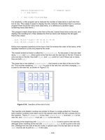
Viewing Different Nodes




In the zoomed-in view you can always see all the nodes in the top two rows: there's only
one, the root, in the top row, and only four in the second row. Below the second row
things get more complicated because there are too many nodes to fit on the screen: 16
on the third row, 64 on the fourth. However, you can see any node you want by clicking

on its parent, or sometimes its grandparent and then its parent.





A blue triangle at the bottom of a node shows where a child is connected to a node. If a


- 343 -
node's children are currently visible, the lines to the children can be seen running from
the blue triangles to them. If the children aren't currently visible, there are no lines, but
the blue triangles indicate that the node nevertheless has children. If you click on the
parent node, its children and the lines to them will appear. By clicking the appropriate
nodes you can navigate all over the tree.




For convenience, all the nodes are numbered, starting with 0 at the root and continuing
up to 85 for the node on the far right of the bottom row. The numbers are displayed to the
upper right of each node, as shown in Figure 10.8.
Nodes are numbered whether they
exist or not, so the numbers on existing nodes probably won't be contiguous.





Figure 10.10 shows a small tree with four nodes in the third row. The user has clicked on

node 1, so its two children, numbered 5 and 6, are visible.










Figure 10.10: Selecting the leftmost children






If the user clicks on node 2, its children 9 and 10 will appear, as shown in Figure 10.11.









Figure 10.11: Selecting the rightmost children

These figures show how to switch among different nodes in the third row by clicking
nodes in the second row. To switch nodes in the fourth row you'll need to click first on a
grandparent in the second row, then on a parent in the third row.





During searches and insertions with the Find and Ins buttons, the view will change
automatically to show the node currently being pointed to by the red arrow.





Experiments




The Tree234 Workshop applet offers a quick way to learn about 2-3-4 trees. Try inserting
items into the tree. Watch for node splits. Stop before one is about to happen, and figure