Data Structures & Algorithms in Java PHẦN 9 docx

- 425 -

for(int m=0; m<currentSize; m++)



if(heapArray[m] != null)



System.out.print( heapArray[m].iData + " ");



else



System.out.print( " ");



System.out.println();



// heap format

int nBlanks = 32;



int itemsPerRow = 1;



int column = 0;



int j = 0; // current item



String dots = " ";



System.out.println(dots+dots); // dotted top line





while(currentSize > 0) // for each heap item

{



if(column == 0) // first item in row?



for(int k=0; k<nBlanks; k++) // preceding blanks



System.out.print(' ');



// display item



System.out.print(heapArray[j].iData);





if(++j == currentSize) // done?

break;





if(++column==itemsPerRow) // end of row?



{



nBlanks /= 2; // half the blanks



itemsPerRow *= 2; // twice the items



column = 0; // start over on



System.out.println(); // new row

}



else // next item on row



for(int k=0; k<nBlanks*2-2; k++)



System.out.print(' '); // interim blanks



} // end for



System.out.println("\n"+dots+dots); // dotted bottom line



} // end displayHeap()




//

-




} // end class Heap




////////////////////////////////////////////////////////////////




class HeapApp



{



public static void main(String[] args) throws IOException



{

int value, value2;



Heap theHeap = new Heap(31); // make a Heap; max size 31



boolean success;





- 426 -

theHeap.insert(70); // insert 10 items



theHeap.insert(40);



theHeap.insert(50);



theHeap.insert(20);

theHeap.insert(60);



theHeap.insert(100);



theHeap.insert(80);



theHeap.insert(30);



theHeap.insert(10);



theHeap.insert(90);





while(true) // until [Ctrl]-[C]

{



putText("Enter first letter of ");



putText("show, insert, remove, change: ");



int choice = getChar();



switch(choice)



{



case 's': // show

theHeap.displayHeap();



break;



case 'i': // insert



putText("Enter value to insert: ");



value = getInt();



success = theHeap.insert(value);



if( !success )



putText("Can't insert; heap is full" + '\n');

break;



case 'r': // remove



if( !theHeap.isEmpty() )



theHeap.remove();



else



putText("Can't remove; heap is empty" +
'\n');




break;

case 'c': // change



putText("Enter index of item: ");



value = getInt();



putText("Enter new priority: ");



value2 = getInt();



success = theHeap.change(value, value2);



if( !success )

putText("Can't change; invalid index" +
'\n');




break;



default:



putText("Invalid entry\n");



} // end switch



} // end while



} // end main()

//
-




- 427 -

public static void putText(String s)



{



System.out.print(s);



System.out.flush();



}

//



public static String getString() throws IOException



{



InputStreamReader isr = new InputStreamReader(System.in);



BufferedReader br = new BufferedReader(isr);



String s = br.readLine();



return s;



}

//



public static char getChar() throws IOException



{



String s = getString();



return s.charAt(0);



}




//

public static int getInt() throws IOException



{



String s = getString();



return Integer.parseInt(s);



}




//




} // end class HeapApp

The array places the heap's root at index 0. Some heap implementations start the array
with the root at 1, using position 0 as a sentinel value with the largest possible key. This
saves an instruction in some of the algorithms, but complicates things conceptually.





The main() routine in HeapApp creates a heap with a maximum size of 31 (dictated by
the limitations of the display routine) and inserts into it 10 nodes with random keys. Then
it enters a loop in which the user can enter s, i, r, or c, for show, insert, remove, or
change.





Here's some sample interaction with the program:




Enter first letter of show, insert, remove, change: s

heapArray: 100 90 80 30 60 50 70 20 10 40









100




90 80



- 428 -


30 60 50 70




20 10 40

Enter first letter of show, insert, remove, change: i




Enter value to insert: 53




Enter first letter of show, insert, remove, change: s




heapArray: 100 90 80 30 60 50 70 20 10 40 53

100




90 80




30 60 50 70




20 10 40 53









Enter first letter of show, insert, remove, change: r

Enter first letter of show, insert, remove, change: s




heapArray: 90 60 80 30 53 50 70 20 10 40









90




60 80




30 53 50 70

20 10 40









Enter first letter of show, insert, remove, change:




The user displays the heap, adds an item with a key of 53, shows the heap again,
removes the item with the greatest key, and shows the heap a third time. The show()
routine displays both the array and the tree versions of the heap. You'll need to use your
imagination to fill in the connections between nodes.





Expanding the Heap Array

- 429 -


What happens if, while a program is running, too many items are inserted for the size of
the heap array? A new array can be created, and the data from the old array copied into
it. (Unlike the situation with hash tables, changing the size of a heap doesn't require
reordering the data.) The copying operation takes linear time, but enlarging the array size
shouldn't be necessary very often, especially if the array size is increased substantially
each time it's expanded (by doubling it, for example).





In Java, a Vector class object could be used instead of an array; vectors can be
expanded dynamically.





Efficiency of Heap Operations




For a heap with a substantial number of items, it's the trickle-up and trickle-down
algorithms that are the most time-consuming parts of the operations we've seen. These
algorithms spend time in a loop, repeatedly moving nodes up or down along a path. The

number of copies necessary is bounded by the height of the heap; if there are five levels,
four copies will carry the "hole" from the top to the bottom. (We'll ignore the two moves
used to transfer the end node to and from temporary storage; they're always necessary
so they require constant time.)





The trickleUp() method has only one major operation in its loop: comparing the key
of the new node with the node at the current location. The trickleDown() method
needs two comparisons, one to find the largest child, and a second to compare this child
with the "last" node. They must both copy a node from top to bottom or bottom to top to
complete the operation.





A heap is a special kind of binary tree, and as we saw in Chapter 8, the number of levels L
in a binary tree equals log
2(N+1), where N is the number of nodes. The trickleUp() and
trickleDown() routines cycle through their loops L–1 times, so the first takes time
proportional to log
2N, and the second somewhat more because of the extra comparison.
Thus the heap operations we've talked about here all operate in O(logN) time.


Heapsort

The efficiency of the heap data structure lends itself to a surprisingly simple and very
efficient sorting algorithm called heapsort.





The basic idea is to insert the unordered items into a heap using the normal insert()
routine. Repeated application of the remove() routine will then remove the items in
sorted order. Here's how that might look:





for(j=0; j<size; j++)



theHeap.insert( anArray[j] ); // from unsorted array



for(j=0; j<size; j++)

anArray[j] = theHeap.remove(); // to sorted array




Because insert() and remove() operate in O(logN) time, and each must be applied
N times, the entire sort requires O(N*logN) time, which is the same as quicksort.
However, it's not quite as fast as quicksort. Partly this is because there are more
operations in the inner while loop in trickleDown() than in the inner loop in
quicksort.





However, several tricks can make heapsort more efficient. The first saves time, and the
second saves memory.





Trickling Down in Place



- 430 -


If we insert N new items into a heap, we apply the trickleUp() method N times.

However, if all the items are already in an array, they can be rearranged into a heap with
only N/2 applications of trickleDown(). This offers a small speed advantage.





Two Correct Subheaps Make a Correct Heap




To see how this works, you should know that trickleDown() will create a correct heap
if, when an out-of-order item is placed at the root, both the child subheaps of this root are
correct heaps. (The root can itself be the root of a subheap as well as of the entire heap.)
This is shown in Figure 12.8.










Figure 12.8: Both subtrees must be correct

This suggests a way to transform an unordered array into a heap. We can apply
trickleDown() to the nodes on the bottom of the (potential) heap—that is, at the end
of the array—and work our way upward to the root at index 0. At each step the subheaps
below us will already be correct heaps because we already applied trickleDown() to
them. After we apply trickleDown() to the root, the unordered array will have been
transformed into a heap.





Notice however that the nodes on the bottom row—those with no children—are already
correct heaps, because they are trees with only one node; they have no relationships to
be out of order. Therefore we don't need to apply trickleDown() to these nodes. We
can start at node N/2–1, the rightmost node with children, instead of N–1, the last node.
Thus we need only half as many trickle operations as we would using insert() N
times. Figure 12.9
shows the order in which the trickle-down algorithm is applied, starting
at node 6 in a 15-node heap.

Figure 12.9: Order of applying trickleDown()






The following code fragment applies trickleDown() to all nodes, except those on the
bottom row, starting at N/2–1 and working back to the root:





for(j=size/2-1; j >=0; j )



- 431 -

theHeap.trickleDown(j);




A Recursive Approach

A recursive approach can also be used to form a heap from an array. A heapify()
method is applied to the root. It calls itself for the root's two children, then for each of
these children's two children, and so on. Eventually it works its way down to the bottom
row, where it returns immediately whenever it finds a node with no children.





Once it has called itself for two child subtrees, heapify() then applies trickleDo
n() to the root of the subtree. This ensures that the subtree is a correct heap. Then
heapify() returns and works on the subtree one level higher.





heapify(int index) // transform array into heap



{



if(index > N/2-1) // if node has no children,

return; // return



heapify(index*2+2); // turn right subtree into heap



heapify(index*2+1); // turn left subtree into heap



trickleDown(index); // apply trickle-down to this node




}




This recursive approach is probably not quite as efficient as the simple loop.




Using the Same Array

Our initial code fragment showed unordered data in an array. This data was then inserted
into a heap, and finally removed from the heap and written back to the array in sorted
order. In this procedure two size-N arrays are required: the initial array and the array
used by the heap.





In fact, the same array can be used both for the heap and for the initial array. This cuts in
half the amount of memory needed for heapsort; no memory beyond the initial array is
necessary.





We've already seen how trickleDown() can be applied to half the elements of an
array to transform them into a heap. We transform the unordered array data into a heap
in place; only one array is necessary for this. Thus the first step in heapsort requires only
one array.





However, things are more complicated when we apply remove() repeatedly to the heap.

Where are we going to put the items that are removed?





Each time an item is removed from the heap, an element at the end of the heap array
becomes empty; the heap shrinks by one. We can put the recently removed item in this
newly freed cell. As more items are removed, the heap array becomes smaller and
smaller, while the array of ordered data becomes larger and larger. Thus with a little
planning it's possible for the ordered array and the heap array to share the same space.
This is shown in Figure 12.10.





- 432 -






FIGURE 12.10: Dual-purpose array

The heapSort.java Program




We can put these two tricks—applying trickleDown() without using insert(), and
using the same array for the initial data and the heap—together in a program that
performs heapsort. Listing 12.2 shows how this looks.





Listing 12.2 The heapSort.java Program




// heapSort.java




// demonstrates heap sort




// to run this program: C>java HeapSortApp

import java.io.*; // for I/O




import java.lang.Integer; // for parseInt()




////////////////////////////////////////////////////////////////




class Node



{



public int iData; // data item (key)

public Node(int key) // constructor



{ iData = key; }



} // end class Node




////////////////////////////////////////////////////////////////




class Heap



{



private Node[] heapArray;

private int maxSize; // size of array



private int currentSize; // number of items in array




//
-




public Heap(int mx) // constructor



- 433 -

{



maxSize = mx;

currentSize = 0;



heapArray = new Node[maxSize];



}




//
-




public Node remove() // delete item with max key



{ // (assumes non-empty list)



Node root = heapArray[0];

heapArray[0] = heapArray[ currentSize];



trickleDown(0);



return root;



} // end remove()




//
-




public void trickleDown(int index)

{



int largerChild;



Node top = heapArray[index]; // save root



while(index < currentSize/2) // not on bottom row



{



int leftChild = 2*index+1;



int rightChild = leftChild+1;



// find larger child

if(rightChild < currentSize && // right ch exists?



heapArray[leftChild].iData <



heapArray[rightChild].iData)



largerChild = rightChild;



else



largerChild = leftChild;



// top >=
largerChild?

if(top.iData >= heapArray[largerChild].iData)



break;



// shift child up



heapArray[index] = heapArray[largerChild];



index = largerChild; // go down



} // end while



heapArray[index] = top; // root to index

} // end trickleDown()




//
-




public void displayHeap()



{



int nBlanks = 32;



int itemsPerRow = 1;



int column = 0;

int j = 0; // current item



String dots = " ";



System.out.println(dots+dots); // dotted top line



- 434 -



while(currentSize > 0) // for each heap item



{



if(column == 0) // first item in row?



for(int k=0; k<nBlanks; k++) // preceding blanks

System.out.print(' ');



// display item



System.out.print(heapArray[j].iData);





if(++j == currentSize) // done?



break;





if(++column==itemsPerRow) // end of row?

{



nBlanks /= 2; // half the blanks



itemsPerRow *= 2; // twice the items



column = 0; // start over on



System.out.println(); // new row



}



else // next item on row



for(int k=0; k<nBlanks*2-2; k++)

System.out.print(' '); // interim blanks



} // end for



System.out.println("\n"+dots+dots); // dotted bottom line



} // end displayHeap()




//
-




public void displayArray()

{



for(int j=0; j<maxSize; j++)



System.out.print(heapArray[j].iData + " ");



System.out.println("");



}




//
-




public void insertAt(int index, Node newNode)

{ heapArray[index] = newNode; }




//
-




public void incrementSize()



{ currentSize++; }




//
-




} // end class Heap

////////////////////////////////////////////////////////////////




class HeapSortApp



{



public static void main(String[] args) throws IOException



- 435 -

{



int size, j;

System.out.print("Enter number of items: ");



size = getInt();



Heap theHeap = new Heap(size);





for(j=0; j<size; j++) // fill array with



{ // random nodes



int random = (int)(java.lang.Math.random()*100);



Node newNode = new Node(random);

theHeap.insertAt(j, newNode);



theHeap.incrementSize();



}





System.out.print("Random: ");



theHeap.displayArray(); // display random array





for(j=size/2-1; j>=0; j ) // make random array into
heap

theHeap.trickleDown(j);





System.out.print("Heap: ");



theHeap.displayArray(); // dislay heap array



theHeap.displayHeap(); // display heap





for(j=size-1; j>=0; j ) // remove from heap and



{ // store at array end



Node biggestNode = theHeap.remove();

theHeap.insertAt(j, biggestNode);



}



System.out.print("Sorted: ");



theHeap.displayArray(); // display sorted array



} // end main()




//
-

public static String getString() throws IOException



{



InputStreamReader isr = new InputStreamReader(System.in);



BufferedReader br = new BufferedReader(isr);



String s = br.readLine();



return s;



}




//

public static int getInt() throws IOException



{



String s = getString();



return Integer.parseInt(s);



}




//


- 436 -
-

} // end class HeapSortApp




The Heap class is much the same as in the heap.java program, except that to save
space we've removed the trickleUp() and insert() methods, which aren't
necessary for heapsort. We've also added an insertAt() method that allows direct
insertion into the heap's array.





Notice that this addition is not in the spirit of object-oriented programming. The Heap
class interface is supposed to shield class users from the underlying implementation of
the heap. The underlying array should be invisible, but insertAt() allows direct access
to it. In this situation we accept the violation of OOP principles because the array is so
closely tied to the heap architecture.





An incrementSize() method is another addition to the heap class. It might seem as
though we could combine this with insertAt(), but when inserting into the array in its
role as an ordered array we don't want to increase the heap size, so we keep these
functions separate.

The main() routine in the HeapSortApp class




1.

Gets the array size from the user.




2.

Fills the array with random data.




3.

Turns the array into a heap with N/2 applications of trickleDown().

4.

Removes the items from the heap and writes them back at the end of the array.




After each step the array contents are displayed. The user selects the array size. Here's
some sample output from heapSort.java:





Enter number of items: 10



Random: 81 6 23 38 95 71 72 39 34 53



Heap: 95 81 72 39 53 71 23 38 34 6

95



81 72



39 53 71 23



38 34 6








Sorted: 6 23 34 38 39 53 71 72 81 95




The Efficiency of Heapsort

As we noted, heapsort runs in O(N*logN) time. Although it may be slightly slower than
quicksort, an advantage over quicksort is that it is less sensitive to the initial distribution of
data. Certain arrangements of key values can reduce quicksort to slow O(N
2
) time,
whereas heapsort runs in O(N*logN) time no matter how the data is distributed.



Summary




•

In an ascending priority queue the item with the largest key (or smallest in a


- 437 -
descending queue) is said to have the highest priority.



•

A priority queue is an Abstract Data Type (ADT) that offers methods for insertion of
data and removal of the largest (or smallest) item.

•

A heap is an efficient implementation of an ADT priority queue.




•

A heap offers removal of the largest item, and insertion, in O(N*logN) time.




•

The largest item is always in the root.




•

Heaps do not support ordered traversal of the data, locating an item with a specific
key, or deletion.

•

A heap is usually implemented as an array representing a complete binary tree. The
root is at index 0 and the last item at index N–1.





•

Each node has a key less than its parents and greater than its children.




•

An item to be inserted is always placed in the first vacant cell of the array, and then
trickled up to its appropriate position.




•

When an item is removed from the root, it's replaced by the last item in the array,
which is then trickled down to its appropriate position.





•

The trickle-up and trickle-down processes can be thought of as a sequence of swaps,
but are more efficiently implemented as a sequence of copies.




•

The priority of an arbitrary item can be changed. First its key is changed; then, if the
key was increased, the item is trickled up, while if the key was decreased the item is
trickled down.





•

Heapsort is an efficient sorting procedure that requires O(N*logN) time.

•

Conceptually heapsort consists of making N insertions into a heap, followed by N
removals.





•

Heapsort can be made to run faster by applying the trickle-down algorithm directly to
N/2 items in the unsorted array, rather than inserting N items.




•

The same array can be used for the initial unordered data, for the heap array, and for
the final sorted data. Thus heapsort requires no extra memory.





- 438 -

Part V




Chapter List




Chapter
13:

Graphs




Chapter
14:

Weighted Graphs




Chapter
15:

When to Use What


Chapter 13: Graphs




Overview




Graphs are one of the most versatile structures used in computer programming. The
sorts of problems that graphs can help solve are generally quite different from those
we've dealt with thus far in this book. If you're dealing with general kinds of data storage
problems, you probably won't need a graph, but for some problems—and they tend to be
interesting ones—a graph is indispensable.





Our discussion of graphs is divided into two chapters. In this chapter we'll cover the
algorithms associated with unweighted graphs, show some algorithms that these graphs
can represent, and present two Workshop applets to model them. In the next chapter
we'll
look at the more complicated algorithms associated with weighted graphs.

Introduction to Graphs




Graphs are data structures rather like trees. In fact, in a mathematical sense, a tree is a
kind of graph. In computer programming, however, graphs are used in different ways
than trees.





The data structures examined previously in this book have an architecture dictated by the
algorithms used on them. For example, a binary tree is shaped the way it is because that
shape makes it easy to search for data and insert new data. The edges in a tree
represent quick ways to get from node to node.





Graphs, on the other hand, often have a shape dictated by a physical problem. For
example, nodes in a graph may represent cities, while edges may represent airline flight
routes between the cities. Another more abstract example is a graph representing the
individual tasks necessary to complete a project. In the graph, nodes may represent
tasks, while directed edges (with an arrow at one end) indicate which task must be
completed before another. In both cases, the shape of the graph arises from the specific
real-world situation.

Before going further, we must mention that, when discussing graphs, nodes are called
vertices (the singular is vertex). This is probably because the nomenclature for graphs is
older than that for trees, having arisen in mathematics centuries ago. Trees are more
closely associated with computer science.





Definitions




Figure 13.1-a shows a simplified map of the freeways in the vicinity of San Jose,
California. Figure 13.1-b shows a graph that models these freeways.



- 439 -

Figure 13.1: Road map and graph






In the graph, circles represent freeway interchanges and straight lines connecting the
circles represent freeway segments. The circles are vertices, and the lines are edges.
The vertices are usually labeled in some way—often, as shown here, with letters of the
alphabet. Each edge is bounded by the two vertices at its ends.





The graph doesn't attempt to reflect the geographical positions shown on the map; it
shows only the relationships of the vertices and the edges—that is, which edges are
connected to which vertex. It doesn't concern itself with physical distances or directions.
Also, one edge may represent several different route numbers, as in the case of the edge
from I to H, which involves routes 101, 84, and 280. It's the connectedness (or lack of it)

of one intersection to another that's important, not the actual routes.





Adjacency




Two vertices are said to be adjacent to one another if they are connected by a single
edge. Thus in Figure 13.1
, vertices I and G are adjacent, but vertices I and F are not. The
vertices adjacent to a given vertex are sometimes said to be its neighbors. For example,
the neighbors of G are I, H, and F.





Paths




A path is a sequence of edges. Figure 13.1 shows a path from vertex B to vertex J that
passes through vertices A and E. We can call this path BAEJ. There can be more than
one path between two vertices; another path from B to J is BCDJ.

Connected Graphs




A graph is said to be connected if there is at least one path from every vertex to every
other vertex, as in the graph in Figure 13.2-a. However, if "You can't get there from here"
(as Vermont farmers traditionally tell city slickers who stop to ask for directions), the


- 440 -
graph is not connected, as in Figure 13.2-b.



A non-connected graph consists of several connected components. In Figure 13.2-b, A
and B are one connected component, and C and D are another.





For simplicity, the algorithms we'll be discussing in this chapter are written to apply to
connected graphs, or to one connected component of a non-connected graph. If
appropriate, small modifications will usually enable them to work with non-connected
graphs as well.

Directed and Weighted Graphs




The graphs in Figures 13.1 and 13.2 are non-directed graphs. That means that the edges
don't have a direction; you can go either way on them. Thus you can go from vertex A to
vertex B, or from vertex B to vertex A, with equal ease. (This models freeways
appropriately, because you can usually go either way on a freeway.)





However, graphs are often used to model situations in which you can go in only one
direction along an edge; from A to B but not from B to A, as on a one-way street. Such a
graph is said to be directed. The allowed direction is typically shown with an arrowhead at
the end of the edge.





In some graphs, edges are given a weight, a number that can represent the physical
distance between two vertices, or the time it takes to get from one vertex to another, or

how much it costs to travel from vertex to vertex (on airline routes, for example). Such
graphs are called weighted graphs. We'll explore them in the next chapter.





We're going to begin this chapter by discussing simple undirected, unweighted graphs;
later we'll explore directed unweighted graphs.




We have by no means covered all the definitions that apply to graphs; we'll introduce
more as we go along.











Figure 13.2: onnected and nonconnected graphs

Historical Note




One of the first mathematicians to work with graphs was Leonhard Euler in the early 18th
century. He solved a famous problem dealing with the bridges in the town of Königsberg,
Poland. This town included an island and seven bridges, as shown in Figure 13.3-a.





- 441 -






Figure 13.3: The bridges of Königsberg

The problem, much discussed by the townsfolk, was to find a way to walk across all
seven bridges without recrossing any of them. We won't recount Euler's solution to the
problem; it turns out that there is no such path. However, the key to his solution was to
represent the problem as a graph, with land areas as vertices and bridges as edges, as
shown in Figure 13.3-b. This is perhaps the first example of a graph being used to
represent a problem in the real world.





Representing a Graph in a Program




It's all very well to think about graphs in the abstract, as Euler and other mathematicians
did until the invention of the computer, but we want to represent graphs by using a
computer. What sort of software structures are appropriate to model a graph? We'll look
at vertices first, and then at edges.





Vertices

In a very abstract graph program you could simply number the vertices 0 to N–1 (where
N is the number of vertices). You wouldn't need any sort of variable to hold the vertices,
because their usefulness would result from their relationships with other vertices.





In most situations, however, a vertex represents some real-world object, and the object
must be described using data items. If a vertex represents a city in an airline route
simulation, for example, it may need to store the name of the city, its altitude, its location,
and other such information. Thus it's usually convenient to represent a vertex by an
object of a vertex class. Our example programs store only a letter (like A), used as a label
for identifying the vertex, and a flag for use in search algorithms, as we'll see later. Here's
how the Vertex class looks:





class Vertex



{



public char label; // label (e.g. 'A')

public boolean wasVisited;





public Vertex(char lab) // constructor



{



label = lab;



wasVisited = false;



}




} // end class Vertex

Vertex objects can be placed in an array and referred to using their index number. In our


- 442 -
examples we'll store them in an array called vertexList. The vertices might also be
placed in a list or some other data structure. Whatever structure is used, this storage is
for convenience only. It has no relevance to how the vertices are connected by edges.
For this, we need another mechanism.




Edges




In Chapter 9, "Red-Black Trees," we saw that a computer program can represent trees in
several ways. Mostly we examined trees in which each node contained references to its
children, but we also mentioned that an array could be used, with a node's position in the
array indicating its relationship to other nodes. Chapter 12, "Heaps,
" described arrays
used to represent a kind of tree called a heap.

A
graph, however, doesn't usually have the same kind of fixed organization as a tree. In a
binary tree, each node has a maximum of two children, but in a graph each vertex may
be connected to an arbitrary number of other vertices. For example, in Figure 13.2-a
,
vertex A is connected to three other vertices, whereas C is connected to only one.





To model this sort of free-form organization, a different approach to representing edges is
preferable to that used for trees. Two methods are commonly used for graphs:the
adjacency matrix and the adjacency list. (Remember that one vertex is said to be
adjacent to another if they're connected by a single edge.)





The Adjacency Matrix




An adjacency matrix is a two-dimensional array in which the elements indicate whether
an edge is present between two vertices. If a graph has N vertices, the adjacency matrix
is an NxN array. Table 13.1 shows the adjacency matrix for the graph in Figure 13.2-a.

Table 13.1: Adjacency Matrix











A




B


C


D

A



0




1


1


1

B



1




0


0


1





C



1

0


0


0





D



1




1


0


0

The vertices are used as headings for both rows and columns. An edge between two
vertices is indicated by a 1; the absence of an edge is a 0. (You could also use Boolean
true/false values.) As you can see, vertex A is adjacent to all three other vertices, B is
adjacent to A and D, C is adjacent only to A, and D is adjacent to A and B. In this
example, the "connection" of a vertex to itself is indicated by 0, so the diagonal from
upper-left to lower-right, A-A to D-D, which is called the identity diagonal, is all 0s. The
entries on the identity diagonal don't convey any real information, so you can equally well
put 1s along it, if that's more convenient in your program.





Note that the triangular-shaped part of the matrix above the identity diagonal is a mirror


- 443 -
image of the part below; both triangles contain the same information. This redundancy
may seem inefficient, but there's no convenient way to create a triangular array in most
computer languages, so it's simpler to accept the redundancy. Consequently, when you
add an edge to the graph, you must make two entries in the adjacency matrix rather than

one.




The Adjacency List




The other way to represent edges is with an adjacency list. The list in adjacency list
refers to a linked list of the kind we examined in Chapter 6, "Recursion." Actually, an
adjacency list is an array of lists (or a list of lists). Each individual list shows what vertices
a given vertex is adjacent to. Table 13.2 shows the adjacency lists for the graph of Figure
13.2-a.




Table 13.2: Adjacency Lists

Vertex


List Containing Adjacent Vertices











A


B  C  D





B


A  D

C


A





D


A  B











In this table, the  symbol indicates a link in a linked list. Each link in the list is a vertex.
Here the vertices are arranged in alphabetical order in each list, although that's not really
necessary. Don't confuse the contents of adjacency lists with paths. The adjacency list

shows which vertices are adjacent to—that is, one edge away from—a given vertex, not
paths from vertex to vertex.





Later we'll discuss when to use an adjacency matrix as opposed to an adjacency list. The
workshop applets shown in this chapter all use the adjacency matrix approach, but
sometimes the list approach is more efficient.





Adding Vertices and Edges to a Graph




To add a vertex to a graph, you make a new vertex object with new and insert it into your
vertex array, vertexList. In a real-world program a vertex might contain many data
items, but for simplicity we'll assume that it contains only a single character. Thus the
creation of a vertex looks something like this:





vertexList[nVerts++] = new Vertex('F');

This inserts a vertex F, where nVerts is the number of vertices currently in the graph.




How you add an edge to a graph depends on whether you're using an adjacency matrix
or adjacency lists to represent the graph. Let's say that you're using an adjacency matrix
and want to add an edge between vertices 1 and 3. These numbers correspond to the


- 444 -
array indices in vertexList where the vertices are stored. When you first created the
adjacency matrix adjMat, you filled it with 0s. To insert the edge, you say




adjMat[1][3] = 1;



adjMat[3][1] = 1;

If you were using an adjacency list, you would add a 1 to the list for 3, and a 3 to the list
for 1.





The Graph Class




Let's look at a class Graph that contains methods for creating a vertex list and an
adjacency matrix, and for adding vertices and edges to a Graph object:





class Graph



{



private final int MAX_VERTS = 20;

private Vertex vertexList[]; // array of vertices



private int adjMat[][]; // adjacency matrix



private int nVerts; // current number of vertices




//
-




public Graph() // constructor



{



vertexList = new Vertex[MAX_VERTS];

// adjacency matrix



adjMat = new int[MAX_VERTS][MAX_VERTS];



nVerts = 0;



for(int j=0; j<MAX_VERTS; j++) // set adjacency



for(int k=0; k<MAX_VERTS; k++) // matrix to 0



adjMat[j][k] = 0;



} // end constructor

//
-




public void addVertex(char lab) // argument is label



{



vertexList[nVerts++] = new Vertex(lab);



}




//
-

public void addEdge(int start, int end)



{



adjMat[start][end] = 1;



adjMat[end][start] = 1;



}




//
-




public void displayVertex(int v)

{



System.out.print(vertexList[v].label);



- 445 -

}




//
-





} // end class Graph




Within the Graph class, vertices are identified by their index number in vertexList.

We've already discussed most of the methods shown here. To display a vertex, we
simply print out its one-character label.




The adjacency matrix (or the adjacency list) provides information that is local to a given
vertex. Specifically, it tells you which vertices are connected by a single edge to a given
vertex. To answer more global questions about the arrangement of the vertices, we must
resort to various algorithms. We'll begin with searches.



Searches




One of the most fundamental operations to perform on a graph is finding which vertices
can be reached from a specified vertex. For example, imagine trying to find out how
many towns in the United States can be reached by passenger train from Kansas City
(assuming that you don't mind changing trains). Some towns could be reached. Others
couldn't be reached because they didn't have passenger rail service. Possibly others
couldn't be reached, even though they had rail service, because their rail system (the
narrow-gauge Hayfork-Hicksville RR, for example) didn't connect with the standard-
gauge line you started on or any of the lines that could be reached from your line.

Here's another situation in which you might need to find all the vertices reachable from a
specified vertex. Imagine that you're designing a printed circuit board, like the ones inside
your computer. (Open it up and take a look!) Various components—mostly integrated
circuits (ICs)—are placed on the board, with pins from the ICs protruding through holes in
the board. The ICs are soldered in place, and their pins are electrically connected to
other pins by traces—thin metal lines applied to the surface of the circuit board, as shown
in Figure 13.4. (No, you don't need to worry about the details of this figure.)










Figure 13.4: ins and traces on a circuit boardSearches






In a graph, each pin might be represented by a vertex, and each trace by an edge. On a
circuit board there are many electrical circuits that aren't connected to each other, so the

graph is by no means a connected one. During the design process, therefore, it may be
genuinely useful to create a graph and use it to find which pins are connected to the
same electrical circuit.





Assume that you've created such a graph. Now you need an algorithm that provides a
systematic way to start at a specified vertex, and then move along edges to other
vertices, in such a way that when it's done you are guaranteed that it has visited every


- 446 -
vertex that's connected to the starting vertex. Here, as it did in Chapter 8, "Binary Trees,"
when we discussed binary trees, visit means to perform some operation on the vertex,
such as displaying it.




There are two common approaches to searching a graph: depth-first search (DFS) and
breadth-first search (BFS). Both will eventually reach all connected vertices. The
difference is that the depth-first search is implemented with a stack, whereas the breadth-
first search is implemented with a queue. These mechanisms result, as we'll see, in the
graph being searched in different ways.

Depth-First Search




The depth-first search uses a stack to remember where it should go when it reaches a
dead end. We'll show an example, encourage you to try similar examples with the
GraphN Workshop applet, and then finally show some code that carries out the search.





An Example




We'll discuss the idea behind the depth-first search in relation to Figure 13.5. The
numbers in this figure show the order in which the vertices are visited.

Figure 13.5: Depth-first search






To carry out the depth-first search, you pick a starting point—in this case, vertex A. You
then do three things: visit this vertex, push it onto a stack so you can remember it, and
mark it so you won't visit it again.





Next you go to any vertex adjacent to A that hasn't yet been visited. We'll assume the
vertices are selected in alphabetical order, so that brings up B. You visit B, mark it, and
push it on the stack.





Now what? You're at B, and you do the same thing as before: go to an adjacent vertex
that hasn't been visited. This leads you to F. We can call this process Rule 1.

REMEMBER



Rule 1: If possible, visit an adjacent unvisited vertex, mark it, and push it on the stack.




Applying Rule 1 again leads you to H. At this point, however, you need to do something
else, because there are no unvisited vertices adjacent to H. Here's where Rule 2 comes
in.





REMEMBER



Rule 2: If you can't follow Rule 1, then, if possible, pop a vertex off the stack.




Following this rule, you pop H off the stack, which brings you back to F. F has no
unvisited adjacent vertices, so you pop it. Ditto B. Now only A is left on the stack.

A, however, does have unvisited adjacent vertices, so you visit the next one, C. But C is
the end of the line again, so you pop it and you're back to A. You visit D, G, and I, and
then pop them all when you reach the dead end at I. Now you're back to A. You visit E,


- 447 -
and again you're back to A.



This time, however, A has no unvisited neighbors, so we pop it off the stack. But now
there's nothing left to pop, which brings up Rule 3.





REMEMBER



Rule 3: If you can't follow Rule 1 or Rule 2, you're finished.




Table 13.3 shows how the stack looks in the various stages of this process, as applied to

Figure 13.5.





Table 13.3: Stack Contents During Depth-First Search










Event


Stack

Visit A


A





Visit B


AB





Visit F


ABF





Visit H

ABFH





Pop H


ABF





Pop F


AB





Pop B


A

Visit C


AC





Pop C


A





Visit D


AD

Visit G


ADG





Visit I


ADGI





Pop I


ADG





Pop G

AD





Pop D


A





Visit E


AE





Pop E


A

- 448 -

Pop A





Done













The contents of the stack is the route you took from the starting vertex to get where you
are. As you move away from the starting vertex, you push vertices as you go. As you

move back toward the starting vertex, you pop them. The order in which you visit the
vertices is ABFHCDGIE.





You might say that the depth-first search algorithm likes to get as far away from the
starting point as quickly as possible, and returns only when it reaches a dead end. If you
use the term depth to mean the distance from starting point, you can see where the name
depth-first search comes from.





An Analogy




An analogy you might think about in relation to depth-first search is a maze. The maze—
perhaps one of the people-size ones made of hedges, popular in England—consists of
narrow passages (think of edges) and intersections where passages meet (vertices).





Suppose that someone is lost in the maze. She knows there's an exit and plans to

traverse the maze systematically to find it. Fortunately, she has a ball of string and a
marker pen. She starts at some intersection and goes down a randomly chosen passage,
unreeling the string. At the next intersection, she goes down another randomly chosen
passage, and so on, until finally she reaches a dead end.





At the dead end she retraces her path, reeling in the string, until she reaches the
previous intersection. Here she marks the path she's been down so she won't take it
again, and tries another path. When she's marked all the paths leading from that
intersection, she returns to the previous intersection and repeats the process.





The string represents the stack: It "remembers" the path taken to reach a certain point.




The GraphN Workshop Applet and DFS




You can try out the depth-first search with the DFS button in the GraphN Workshop
applet. (The N is for not directed, not weighted.)

Start the applet.
A
t the beginning, there are no vertices or edges, just an empty rectangle.
You create vertices by double-clicking the desired location. The first vertex is
automatically labeled A, the second one is B, and so on. They're colored randomly.





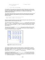
To make an edge, drag from one vertex to another. Figure 13.6 shows the graph of
Figure 13.5 as it looks when created using the applet.








- 449 -


Figure 13.6: The GraphN Workshop applet

There's no way to delete individual edges or vertices, so if you make a mistake, you'll
need to start over by clicking the New button, which erases all existing vertices and
edges. (It warns you before it does this.) Clicking the View button switches you to the
adjacency matrix for the graph you've made, as shown in Figure 13.7. Clicking View
again switches you back to the graph.










Figure 13.7: Adjacency matrix view in GraphNSearches






To run the depth-first search algorithm, click the DFS button repeatedly. You'll be
prompted to click (not double-click) the starting vertex at the beginning of the process.

You can re-create the graph of Figure 13.6, or you can create simpler or more complex
ones of your own. After you play with it a while, you can predict what the algorithm will do
next (unless the graph is too weird).





If you use the algorithm on an unconnected graph, it will find only those vertices that are
connected to the starting vertex.




Java Code




A key to the DFS algorithm is being able to find the vertices that are unvisited and
adjacent to a specified vertex. How do you do this? The adjacency matrix is the key. By
going to the row for the specified vertex and stepping across the columns, you can pick
out the columns with a 1; the column number is the number of an adjacent vertex. You
can then check whether this vertex is unvisited. If so, you've found what you want—the
next vertex to visit. If no vertices on the row are simultaneously 1 (adjacent) and also
unvisited, then there are no unvisited vertices adjacent to the specified vertex. We put the
code for this process in the getAdjUnvisitedVertex() method:

// returns an unvisited vertex adjacent to v



public int getAdjUnvisitedVertex(int v)



{



for(int j=0; j<nVerts; j++)



if(adjMat[v][j]==1 && vertexList[j].wasVisited==false)



return j; // return first such vertex



return -1; // no such vertices

} // end getAdjUnvisitedVert()